Abstract
This paper provides a comprehensive overview of approaches to the determination of isocontours and isosurfaces from given data sets. Different algorithms are reported in the literature for this purpose, which originate from various application areas, such as computer graphics or medical imaging procedures. In all these applications, the challenge is to extract surfaces with a specific isovalue from a given characteristic, so called isosurfaces. These different application areas have given rise to solution approaches that all solve the problem of isocontouring in their own way. Based on the literature, the following four dominant methods can be identified: the marching cubes algorithms, the tessellation-based algorithms, the surface nets algorithms and the ray tracing algorithms. With regard to their application, it can be seen that the methods are mainly used in the fields of medical imaging, computer graphics and the visualization of simulation results. In our work, we provide a broad and compact overview of the common methods that are currently used in terms of isocontouring with respect to certain criteria and their individual limitations. In this context, we discuss the individual methods and identify possible future research directions in the field of isocontouring.
Keywords:
isocontours; isosurfaces; isocontouring; level set; contour lines; computer graphics; image processing; marching cubes; marching tetrahedra; surface nets; ray tracing; tessellation MSC:
65D17; 65D18; 68U05
1. Introduction
In many scientific areas, one is interested in identifying, from a set of given data, those that have a constant value. A classic field of application here is cartography for the representation of lines of different levels. These are represented as so-called contour lines on a two-dimensional plane (in this case, a map). In this context, the contour lines represent height levels that have the same value in relation to a defined reference level. This approach enables information from three-dimensional space to be graphically illustrated in a compact form and the characteristics of the existing data set to be visualized appropriately.
In practice, however, it is easy to see that this type of problem is not limited to geography but can be found in many different areas. These include, for example, medical imaging, image processing or the creation of weather maps. In most cases, three-dimensional or four-dimensional data sets are examined in order to extract two-dimensional isocontours or three-dimensional isosurfaces. Regardless of the particular application, however, the overarching task of iscontour extraction is mathematically identical, which can be defined in principle as follows, based on [1].
Definition 1
(Isocontour extraction). Let and be sets with and corresponding mapping . Consider a given sample set over and a constant value ; then, find the set so that applies. The set is referred to as the isocontour.
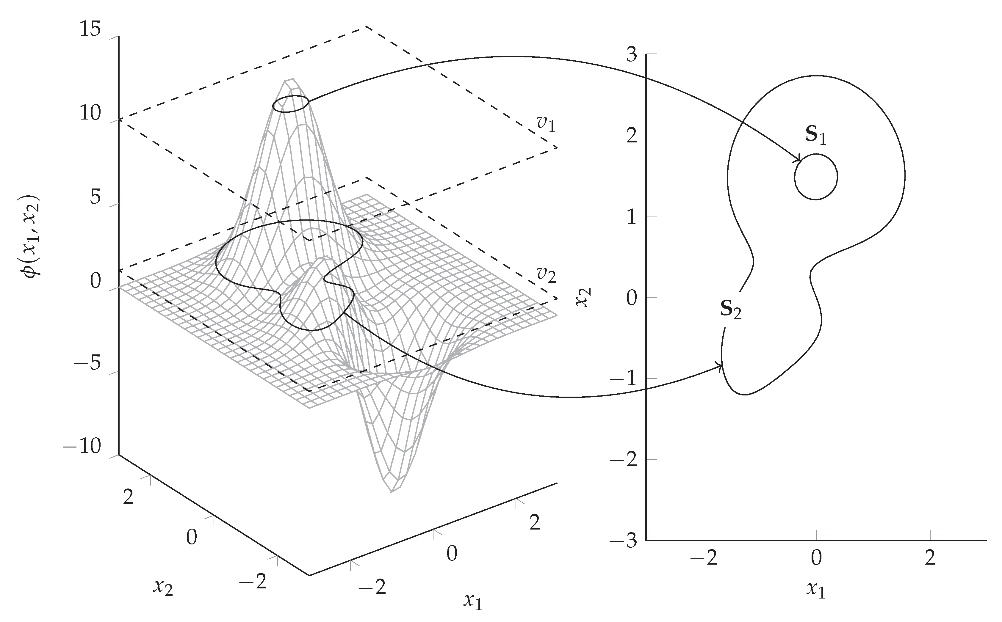
The task described in Definition 1 is qualitatively illustrated in this context in Figure 1.
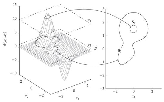
Figure 1.
Exemplary isocontour extraction considering the Peaks function denoted as from MATLAB© for constant values .
For a given mapping (here, the Peaks function of the MATLAB© software environment), the sets and for which , , respectively, applies are to be identified. The results are then the according isocontours.
In our work, we focus on methods that are relevant to the task described in Definition 1 and are referred to as isocontouring methods in the following. When analyzing research carried out in this area, it first becomes apparent that the problem, as described at the beginning, occurs in different application areas. As a result, methods have been developed that solve the isocontouring problem in their own way for each specific application. This is particularly related to the structure of the available data. For example, medical applications often use pixel-based and structured data sets from which isosurfaces must be extracted. In the context of measurement series, on the other hand, unstructured data sets often occur, which require a different solution approach for the extraction of isosurfaces. In addition, the presentation of the results plays an important role in the respective methods used.
Based on our investigations in this area, it can be stated that the methods for isosurface extraction can be classified into four dominant representatives:
- Marching cubes algorithms;
- Tessellation-based algorithms;
- Surface nets algorithms; and
- Ray tracing algorithms.
These groups are the subject of our investigation and will be examined in more detail in the further course of the paper.
2. Marching Squares and Marching Cubes Algorithms
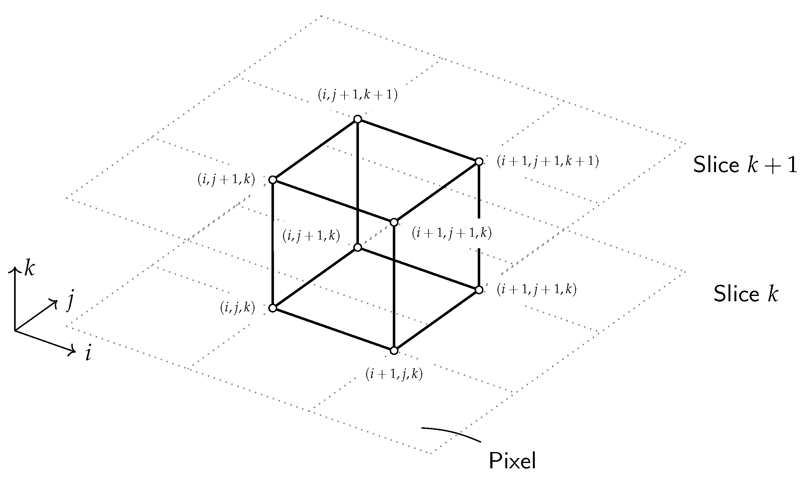
The marching cubes algorithm (MC) was introduced in [2] by W. E. Lorensen and H. E. Cline to find isovalues in medical imaging techniques such as magnetic resonance imaging (MRI), computed tomography scans (CT scan) and single-photon emission computed tomography (SPECT). Therefore, the initial data can be interpreted as pixels in a three-dimensional picture. A schematic representation of the data is shown in Figure 2. The k dimension represents the individual pictures, where the position of each pixel within one slice is represented by i and j. Hence, the cube presented in Figure 2 is constructed by four opposing pixels in two neighboring slices.

Figure 2.
Initial data structure for marching cubes algorithm based on [2].
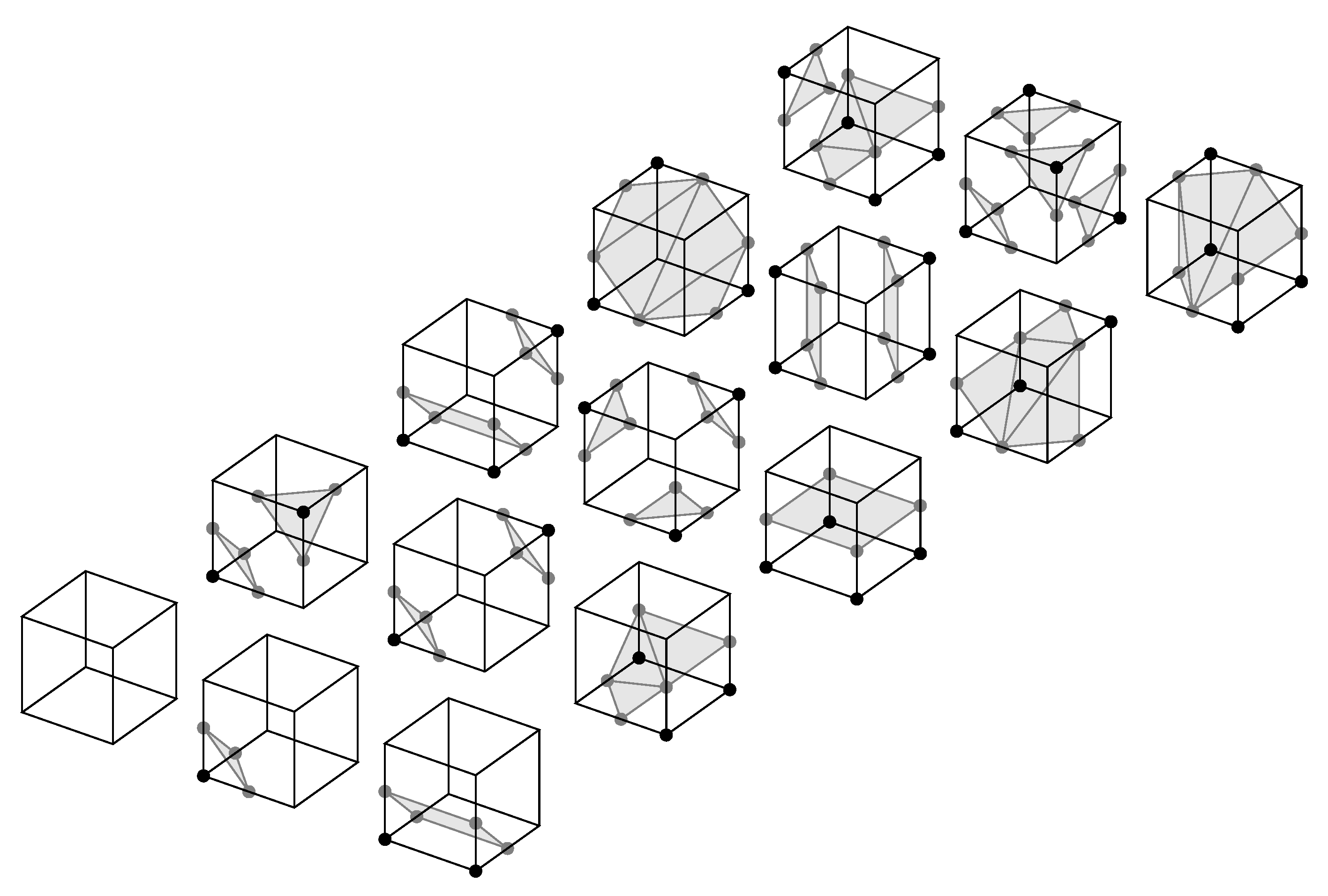
To be able to interpret the data in a medical context, points of equal value must be found. This value can represent a specific tissue density, for example, so that the result of the analysis yields the three-dimensional surface of individual parts of the scan. The marching cubes algorithm follows a divide-and-conquer approach, where each cube is analyzed individually, resulting in small triangles of the surface that, when put together, reconstruct the surface formed by the isovalue. The first step is to mark all vertices of the individual cubes that have a value smaller than, equal to or greater than the isovalue of interest. Since a cube has eight vertices, which themselves can have two states, 256 patterns are possible. Using the symmetries between the individual cases, only 14 different general cases are necessary according to [2]. Cubes where all vertices have values smaller or greater than the isovalue are outside or inside the surface, do not contribute to the surface itself and thus must not be considered in the further process. All other combinations do contribute and are investigated in the following steps. In Figure 3, the different combinations are shown. Here, the highlighted triangles in the individual cubes are part of the surface.

Figure 3.
Basic types of triangulated cubes based on [2].
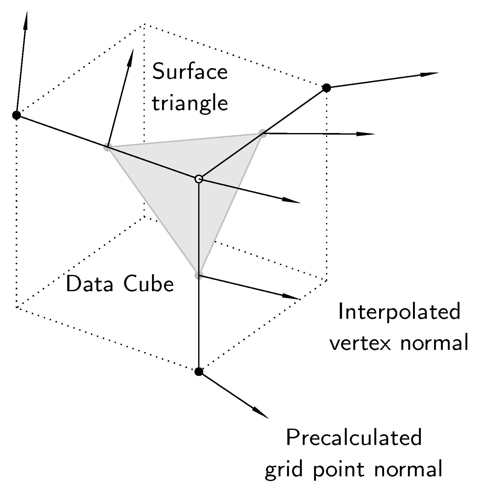
Based on the values of the cube vertices, the position of the point of the isovalue on the edges of the cube can be determined by linear interpolation. The final step of the proposed algorithm uses the interpolated points, the vertices of the cube under investigation and the vertices of the neighboring cubes to calculate the unit normal used for Gourard-shaded images. This is not necessary for the interpolation itself but for the imaging and the subsequent medical analysis. To calculate the unit normal of the density D on each interpolated vertex, first, the normal at the cube vertices is calculated in the x, y and z directions. For this purpose, the density gradient G is calculated, using the expressions presented in Equations (1)–(3). The distance between two pixels in the same slice is and , while the distance between two slices is .
After calculating the gradient at the cube vertices, the gradient at the isovalue vertices can be determined using linear interpolation. Since the component of the gradient vector in the tangential direction of the isovalue surface is always zero, the gradient vector itself represents a normal vector of the respective vertex. In Figure 4, an example is depicted where the gradients of the cube vertices are known and yield the normal unit vectors at the vertices of the isovalue triangle.
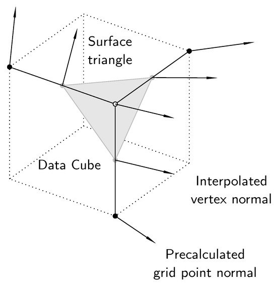
Figure 4.
Unit normal vector calculation at vertices of isovalue surfaces based on [3].
The original marching cubes algorithm is the subject of various other scientific works. Authors P. Shirley and A. Tuchman propose, in [4], a method to decompose the cubes into tetrahedral cells before linearization, to increase the calculation efficiency. A problem in the original algorithm is the ambiguities of the 14 patterns depicted in Figure 3. This eventually leads to erroneous artifacts in the resulting three-dimensional object. The Asymptotic Decider, by G. M. Nielson and B. Hamann, proposed in [5], aims to achieve exact solutions. Hyperbolas are used to determine the exact solutions for ambiguous cases. On the other hand, E. Chernyaev proposes 33 patterns in [6] instead of 14 to fully describe all necessary patterns in the marching cubes 33 algorithm (MC33). In [7], B. K. Natarajan shows the ambiguities of the isosurfaces inside the cubes. To obtain definite solutions, an extension of the original algorithm is proposed that recognizes the shape of the interpolation surface. For this purpose, decision paths are implemented that recognize and correctly assign saddle surfaces. Another approach to deal with erroneous parts in the surface is presented in [8] by X. Wang et al. The improvement is implemented by combining the surface results of adjacent individual cubes to determine the final shape. The algorithm detects common edges and uses this information throughout the whole surface generation process. Further improvements regarding the computation time of the algorithm are proposed by C. Henn et al. in [3]. Instead of calculating and storing the normal unit vectors in Cartesian coordinates, discretized polar coordinates are proposed. Since the length of the normal unit vectors is not needed in the later process, in polar coordinates, only two coordinates are necessary to receive all relevant information. In addition, the use of floating point numbers is omitted and, instead, the discretization of the space angles is proposed to reduce the memory requirements. Z. Xu et al. also introduce improvements to the calculation time in [9] by eliminating linearization and using the centroid of the cubes instead. According to the authors, this is permissible for high-resolution data spaces. In addition, calculations of cube vertices that are already calculated are omitted and edges are combined under special conditions, yielding an overall reduced calculation load. First named by G. Nielson in [10], the dual marching cubes algorithm (DMC) enables a higher resolution of the surface. The triangles created by the original algorithm are used to construct new surface patches. The new patches are formed using the centroids of four adjacent marching cube triangles, forming a new surface mesh. Authors S. Gong and T. S. Newman improve, in [11], the performance for two-dimensional data. R. Grosso and D. Zint enable, in [12], the algorithm to be calculated in parallel. Furthermore, to enable the algorithm to detect sharp edges within a cube, S. Gong and T. S. Newman implement, in [13,14], an extension of the marching cubes algorithm. Neighboring cubes are taken into account to detect sharp edges within one cube and the creation of the isosurface triangles is adopted accordingly. Another problem in the original algorithm is surface construction using too small or sharp triangles. This issue is solved by S. Raman and R. Wenger in [15] by taking cube vertices into account that are equal to the isovalue. This eventually leads to more patterns than the original 14 but yields a more robust surface construction. In [16], L. Custodio et al. apply the same approach to the marching cubes 33 algorithm. A further improvement in the reconstructed surface can be achieved, according to S. Gong and T. S. Newman in [17], by comparing the value of the estimated voxel with the original voxel. If deviations occur, a post-processing step can adjust the estimated voxel so that the original data are matched. Measured data that are subject to noise are the focus of the work of Y. He et al. in [18], where probability theory is used to improve the isovaluing result of noisy input data. Further literature for the marching cubes algorithm can be found in [19], while a compact summary of marching cubes algorithms can be obtained from Table 1.

Table 1.
Summary of marching cubes algorithms.
3. Tessellation-Based Algorithms
Tessellation-based algorithms have their origins in representing the inner surfaces of three-dimensional objects. For the first time, B. A. Payne and A. W. Toga introduced a tessellation-based method in [20], which aims to display the inner surfaces and functions of a human brain. This requires the outer surface, the subcortex, to be removed. To do this, a volume, the so-called minimum distance field, is first determined, where each point within the volume is assigned the minimum distance to the nearest point on the cortical surface as a value. The thresholding of the volume is then performed so that a set of surfaces with a constant minimum distance to the cortex is created. Then, the surface elements generated by thresholding are divided into connected components so that the desired inner surfaces are separated from the surfaces equidistant from the brain. The authors use a modified marching cubes algorithm for thresholding. Since the marching cubes algorithm can lead to ambiguous situations that can lead to topologically unconnected surfaces, each cube is divided into five tetrahedra and each tetrahedron through which the surface passes is then polygonized. As previously mentioned, the basic idea of building cubes of eight pixels each over two neighboring slices is therefore initially based on the marching cubes algorithm. In [20], the authors show that, apart from possible holes at the edges of the sampled field, the method produces topologically correct, closed surfaces that can then be subjected to both quantitative analysis and rendering.
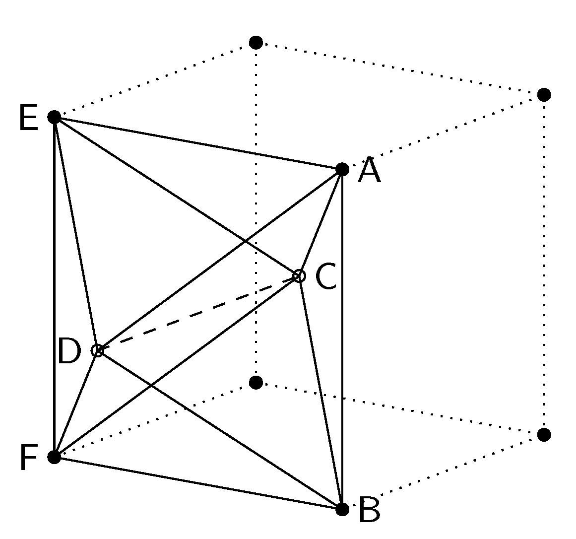
In [21], J. Bloomenthal describes an algorithm for the polygonization of implicit surfaces. In the method, an initial cube is first centered on a surface point and then a new cube is generated on each face that contains corners with opposite polarity. If the entire surface contains cubes, the surface in each cube is approximated by one or two polygons. To do this, the cube is divided into five tetrahedra, which are then polygonized. The polygonization is based on a table that has an entry for every possible configuration. In contrast to the 256 entries with possible configurations in the marching cubes algorithm, there are only 16 entries when using tetrahedra. Each tetrahedral configuration produces either nothing, a triangle or a quadrilateral, i.e., two triangles, as shown in Figure 5.
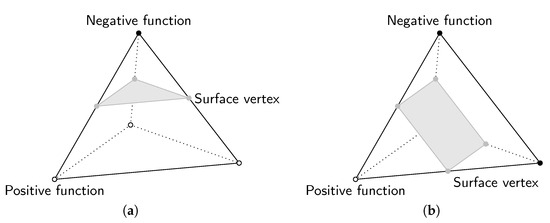
Figure 5.
The two types of possible tetrahedral configurations based on [21]; (a) triangle, (b) quadrilateral.
In [22], A. Guéziec and R. Hummel present an approach, based on the algorithm of B. A. Payne and A. W. Toga, for the fast and efficient extraction and visualization of surfaces defined as isosurfaces in three-dimensional interpolated data. The surface is extracted as a collection of closed triangles, where each triangle is an oriented closed curve within a single tetrahedron. Thus, the entire surface is wrapped with triangles. A. Guéziec and R. Hummel have extended the algorithm in [23,24] in terms of surface simplification and the necessary memory capacity.
Y. Zhou et al. clarify in [25] that, despite the decomposition of the cubes into tetrahedra, the ambiguity problem has not yet been solved. Therefore, the authors propose a method of determining the intersection points and a criterion to test the intersection between the isosurface and the edge of the tetrahedron, which are based on the assumption that the function is linear along the edge of a cube. However, the authors deduce in [25] that there is a quadratic variation in the function value along the triangle edge t, as can be seen in Equation (4).
The values for , and are determined by the function values at the vertices. If one or both zeros of the function
are an element of the interval , the isocontour with the isovalue C intersects the triangle edge. In addition, the connection of intersection points in the tetrahedra to construct the polygons and the triangulation of the polygons are discussed. They show that, with the proposed method, the isosurfaces are independent of the exact distribution of the tetrahedra resulting from the decomposition of the cubes.
In [26], G. M. Nielson and R. Franke present an algorithm that computes a triangulated surface that separates a collection of data points segmented into several different classes instead of only two. The algorithm can be used for both structured, rectilinear and scattered data sets. For tetrahedrization, each cell is decomposed into five or six tetrahedra for structured data sets, while tetrahedrization is assumed for scattered data sets. However, the algorithm assumes that the data are already segmented.
Authors K. S. Bonnell et al. describe, in [27], a new algorithm for the reconstruction of material interfaces from data sets with volume fractions. The algorithm is based on a dual tetrahedral mesh constructed from the original mesh, where each vertex in the dual mesh is assigned an associated barycentric coordinate representing a fraction of each material present. The material boundaries are determined by mapping a tetrahedron into barycentric space and calculating the intersection points with Voronoi cells in barycentric space. These intersections are then mapped back into the original physical space and triangulated to approximate the surface boundary.
The so-called marching tetrahedra algorithm (MT) was developed and improved in parallel to the polygonization method already presented, where cubes are divided into tetrahedra. This method is also based on the basic idea of the marching cubes algorithm, but, unlike the polygonization method described above, it does not first create cubes, which are then divided into triangles, but the grid is divided directly into triangles. In the new method, which was first presented by S. L. Chan and E. O. Purisima in [28], the space is divided directly into tetrahedra to create a regular and symmetrical tessellation. This can be achieved by using a space-centered cubic grid, as shown in Figure 6. In this way, all tetrahedra have the same shape, even if they differ in orientation.

Figure 6.
Tessellation scheme for the marching tetrahedra algorithm based on the space-centered cubic lattice based on [28].
The tetrahedra thus obtained have two different types of edges, the longer ones, i.e., and , and the shorter ones, i.e., , , and , as shown in Figure 6. Each long edge is used in four tetrahedra and each short edge is used in six. In contrast to the 15 ways in which the surface can intersect a cube, there are only four with the tetrahedrons constructed in this way. The first case is that all vertices have the same state and the surface therefore does not intersect the tetrahedron. If one vertex has a different state from the other three, the surface can be constructed parallel to the triangle formed by the three vertices. If two vertices have the same state, there are two ways in which the surface can intersect the tetrahedron, whereby a quadrilateral surface element can be formed for both cases. The two cases are that the identical vertices can be connected either with a short or with a long edge. Another advantage is that the sampling efficiency is improved compared to using the standard cubic grid. However, the space-centered cubic grid is not available per se for applications that include a scan, so the values in the center of each cube must be interpolated.
In [29], S. L. Chan and E. O. Purisima extend the marching tetrahedra algorithm for the generation and triangulation of molecular surfaces. The triangulated surface generated in this way can be used both for molecular graphic display and for boundary element continuum dielectric calculations. T. Lu and F. Chen present, in [30], an algorithm that has been improved in terms of computing time and employ it for a quantitative analysis of molecular surfaces.
As an extension to the original marching tetrahedra algorithm, authors G. M. Treece et al. proposed the regularized marching tetrahedra algorithm in [31]. The method combines the marching tetrahedra algorithm with the vertex clustering algorithm so that isosurfaces are generated that match the data topologically and, at the same time, contain an appropriate number of triangles with improved aspect ratios for the sampling resolution. This significantly reduces the number of triangles used to represent the surface and improves the smooth, shaded representation of the surface. The surface triangulations generated using the method are presented for implicit surfaces, medical data with thresholds and surfaces created from object cross-sections.
In [32], A. Cong et al. propose the mulitregional marching tetrahedra method, which is used for the extraction of surface and volume meshes from segmented CT, micro-CT or MRI image volumes of a small experimental animal. The method is used to extract the triangulated surface mesh and construct a volumetric mesh for all anatomical components within a sweep over all segmented CT slices. Since the volume of all components is meshed with a finite element mesh, it can be used directly for finite element calculations. In addition, compared to the marching tetrahedra method, two further cases are considered during surface extraction within the tetrahedra and a seamless transition between anatomical components is ensured. The surface is then smoothed and simplified without losing the seamless transition. The method is used by the authors in bioluminescence tomography.
In [33], G. M. Nielson presents a further extension of the classical marching tetrahedra method, the dual marching tetrahedra method. The method is a generalization of the cuberille method from cubes to tetrahedra and is used to render surfaces in a three-dimensional space. The dual marching tetrahedra method solves a fundamental problem in the original cuberille method, in which the separating surfaces are not necessarily manifolds. The method can be used for both structured and unstructured point clouds.
V. d’Otreppe et al. use the marching tetrahedra method to generate smooth surface meshes from multi-region medical images. For this purpose, the marching tetrahedra method is extended in [34] for use in multi-domain data, so that multi-region meshes are generated as a set of triangular surface pieces that consistently connect to each other at the material boundaries, combined with a method for the reconstruction of implicit surfaces. With this mesh generation strategy, it is possible to produce surface meshes using triangles from segmented medical data sets with multiple tissues. In addition, the terracing artifacts are avoided by the smooth description of the tissue boundaries before triangulation.
T. Shen et al. pursue a deep learning approach for high-resolution three-dimensional shape synthesis in [35], where the marching tetrahedra method is integrated into the deep learning framework. In the proposed approach, implicit and explicit surface representations are combined and the quality of shape synthesis is improved by the additional supervision defined directly on the extracted surface from the implicit field.
Further research on the use of the marching tetrahedra method in the field of geological modeling can be found in [36,37].
Another approach to determining isocontours in the field of tessellation-based algorithms comprises methods incorporating the triangulation of the point cloud to be analyzed. In [38], C. L. Bajaj et al. present a fast isocontouring algorithm for scalar volume data. In a preprocessing step, seed cells are selected so that at least one cell per connected component of each isocontour is present. For the given isovalue, all cells of the previously defined seed cells that intersect the isocontour are then extracted. This leads to a significant reduction in calculation complexity.
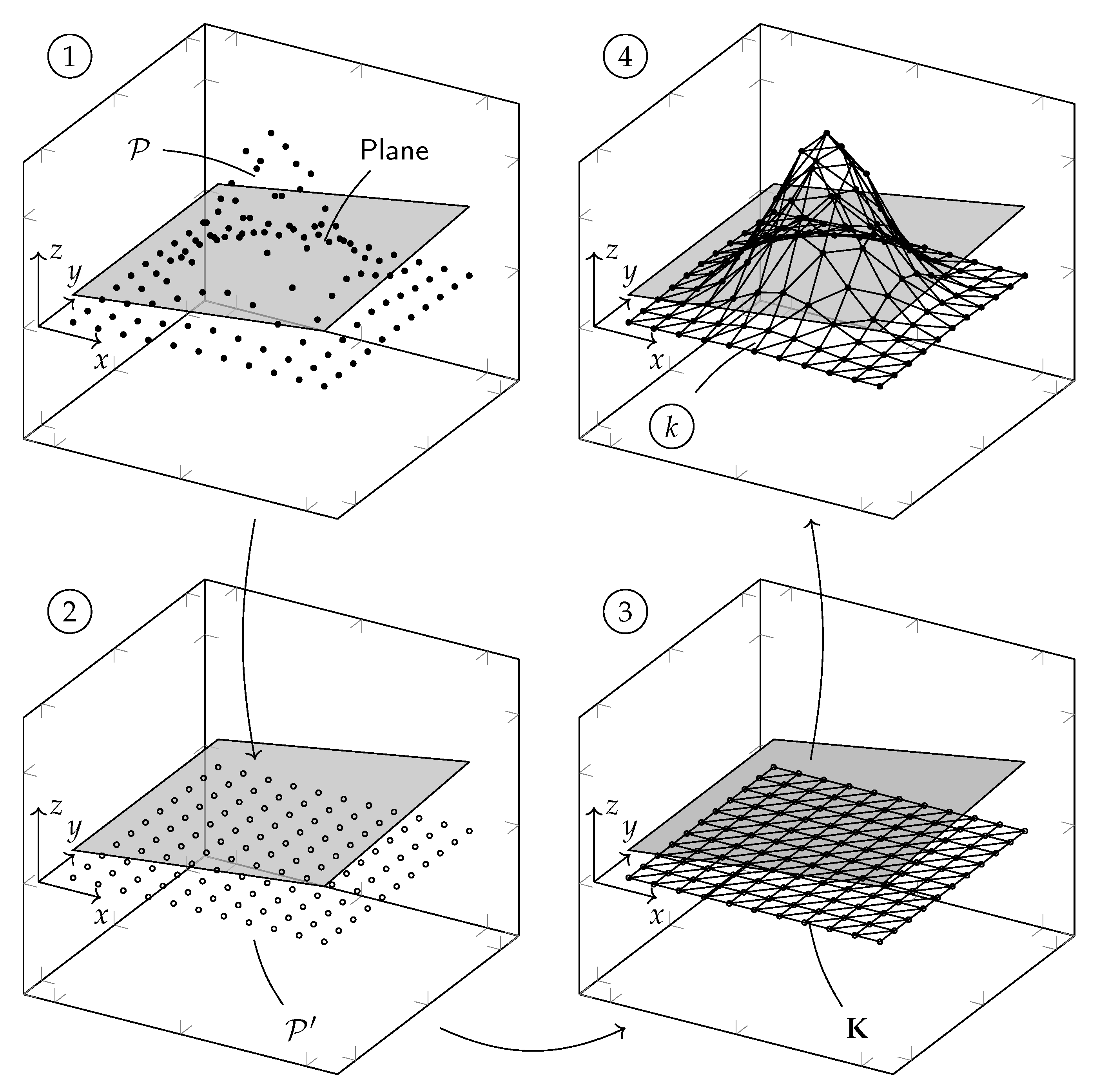
Another mesh-based method of approximating isocontours in a three-dimensional scalar field is the RooTri() function, introduced by J. Oellerich et al. in [39]. A specific feature of the proposed algorithm is that unstructured three-dimensional point clouds can be processed. Furthermore, intersection points with an arbitrarily oriented plane can be determined. First, the unstructured three-dimensional point cloud is projected onto a two-dimensional plane so that the third component describing the variable under investigation is neglected for each point. The point cloud is then triangulated using Delaunay triangulation. Subsequently, each triangular vertex, i.e., each point from the point cloud, is again supplemented by the corresponding third component. This creates a three-dimensional, triangulated surface, as shown in Figure 7.

Figure 7.
Basic approach of the RooTri() function from [39]: ➀ three-dimensional point cloud and defined contour level, ➁ projection of the point cloud onto the original plane to obtain the set , ➂ Delaunay triangulation of the point cloud to receive triangle set K, ➃ re-adding the z-component to each triangle vertex .
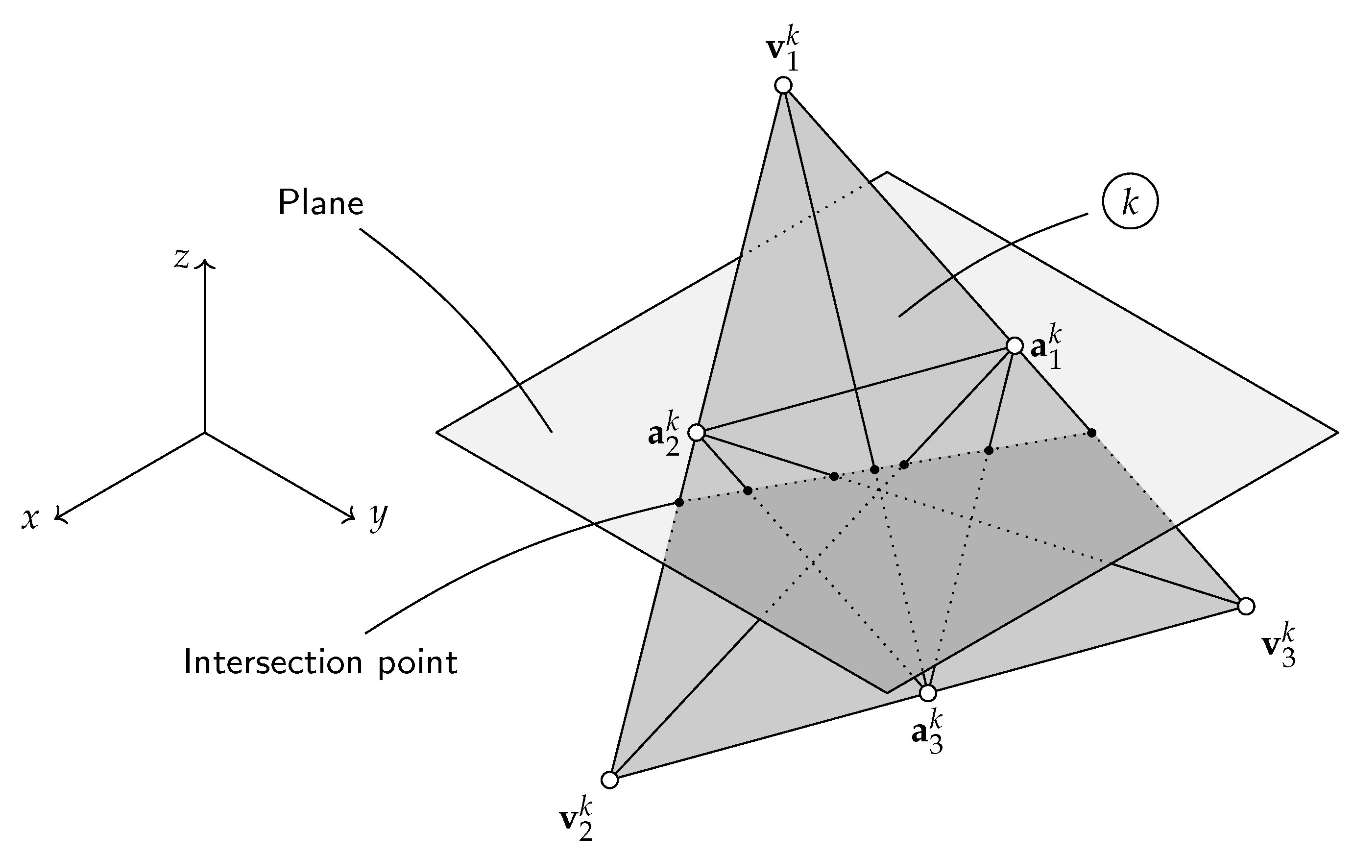
Next, the method verifies whether there is an intersection point with the plane for each triangle generated in this way. To do this, we proceed as shown in Figure 8 for each triangle, interpolating linearly between the vertices , and .

Figure 8.
Calculation of intersection points for each triangle from [39].
Using the vertices (or the edge midpoints ), of the k-th triangle, it is possible to set up the vectors , , as in Equations (5)–(7).
Here, applies. Inserting the plane in coordinate form
and solving for lambda leads to
Substituting from Equation (8) into Equations (5)–(7) results in the coordinates
of the intersection point. If is an element of the interval , it is a valid intersection point. The code is implemented by the authors in vectorized form, which significantly increases the performance of the algorithm, although each triangle must be checked for intersection points. The validity of the algorithm is checked by comparing it with the contourc() function provided by MATLAB©. In addition to the quality of the results obtained, the number of intersections calculated, the time required and the estimated memory requirements are moreover considered for various functions. In addition to the significantly higher quality of the intersection points, RooTri() also has a significantly greater number of intersection points, which simplifies the determination of connected isocontours. Furthermore, RooTri() is, on average, faster than contourc() and requires only half the memory. The use of the algorithm is not limited to the analysis of functions, but it can also be used in the evaluation of unstructured data, such as in measurements. In [39], the algorithm was used to evaluate the measurement results of a permanently excited synchronous machine. Equipotential lines of constant torque were determined. Another use case of the algorithm is topology optimization, which is a subarea of structural optimization. The aim here is to find a suitable material distribution within a given design domain. With the help of RooTri(), zeros of a higher-dimensional scalar function can be determined that correspond to the material boundary.
Research on the extraction and compression of hierarchical isocontours from image data using dynamic tessellation can be reviewed in the papers [40,41] of T. Lewiner et al. In [42], a computational framework for two-dimensional shape-enclosing contours based on the application of Delaunay tessellation is presented by B. R. Schlei. Research on the use of tessellation-based methods for terrain models and topography can be found in [43,44]. A summary of the tessellation-based algorithms cited in this work can be found in Table 2.
Table 2.
Summary of tessellation-based algorithms.
4. Surface Nets Algorithms
The surface nets algorithm was first presented by S. F. F. Gibson in [45] for the creation of a globally smooth surface model from a set of three-dimensional data points. The method is commonly used in computer graphics, e.g., medical imaging, and computational geometry to create smooth surfaces from binary segmented data. The advantage of this method is its simplicity and effectiveness, which makes it a popular choice for the creation of surface models from structured three-dimensional point clouds, such as binary-segmented MRI or CT image volumes. However, it may not always produce the most accurate or detailed meshes, especially in regions with complex geometry or high curvature. Overall, this method follows a similar approach to the marching cubes algorithm in the initial steps. Nevertheless, the two methods differ with regard to the exact determination of the surface area within a cube.
The basic idea of the surface nets algorithm is to link the surface nodes of the binary-segmented volume and relax the node positions within a given dimension in such a way that a smooth surface is generated. The linked surface nodes form the surface nets. To generate the surface net, the first step is to find the surface nodes in the data. To do this, the three-dimensional point cloud is first divided into cubes with eight voxels each. If all eight voxels have the same binary value, this means that the cube is either completely inside or outside the object. If at least one voxel has a different binary value from its neighbors, then the surface travels through this cube. A node is placed in the centroid of all cubes through which the surface travels and connected to the node in the neighboring surface cubes to create the surface net; see Figure 9a. One node can thereby have up to six connections. The positions of the nodes of the surface net are then iteratively relaxed so that an energy measure in the links is reduced. Here, the energy E is determined in [46] by the sum of the length of the connections between the nodes within a surface net, as shown in Equation (9).
Figure 9.
Qualitative illustration of the surface nets algorithm based on [45]. (a) The underlying net with linked surface nodes in the center of each surface cube. (b) The relaxed net with smoothed out terraces. ➀ and ➁ Possible surface constructions for a two-dimensional surface cube with matched diagonal elements, whereby one of the two topologies is selected arbitrarily in marching cubes. ➂ In surface nets, the surface is pinched together at the ambiguous node point.
In this connection, and describe the two linked nodes and n represents all links within a surface net. Subsequently, the total energy is reduced by reducing the length of all links in a surface net and a local minimum of energy is achieved by moving the nodes to a position between two neighboring nodes, as shown in Equation (10) for node i.
The number of neighboring links for node i is described here via . However, a node can only be moved within the surface cube in which it was defined, in order to remain true to the original segmentation; see Figure 9b. This makes it possible to reduce the aliasing and terracing artifacts on the surface. In contrast to the marching cubes algorithm, the surfaces in the surface nets algorithm are not drawn arbitrarily through the surface cubes, which have identical elements at the opposite corners. In marching cubes, there are two different ways in which the surface can run through the cube, which leads to topologically different surfaces; see Figure 9➀,➁. One of the two possibilities is chosen arbitrarily. In surface nets, the surface is pinched at the net node, whereby the surface is neither divided nor connected; see Figure 9➂. Since the topological decision is not made arbitrarily, it is possible that higher-level algorithms can be used to separate or connect the surface at the ambiguous points after smoothing. S. F. F. Gibson shows, in [45], that the surface nets algorithm is capable of generating relatively smooth surfaces for curved objects and sharp corners for rectangular objects, as well as obtaining thin structures and cracks. The smoothed surface net can then be triangulated to create a three-dimensional surface model. To render these surfaces, distance maps are determined from the triangulated surface, which can be determined from the distance of the respective point from the distance map to the next surface triangle. S. F. F. Gibson later patented the approach for the calculation of isosurfaces from binary-segmented data and the subsequent smoothing of these surfaces in [46].
In [47], S. F. F. Gibson used the distance maps generated with the surface nets algorithm to comprehensively demonstrate its quality and effectiveness for surface reconstruction in sampled volumetric data. This is shown primarily using the example of medical images from MRI or CT data. For this purpose, the values for the distance to the nearest surface are mapped to each sample point and the surface is reconstructed using the zero value of the distance map.
M. E. Leventon and S. F. F. Gibson present, in [48], the dual surface nets algorithm, which combines two orthogonal scans. In this way, a model can be generated with a higher resolution than with both scans alone. This reduces the most severe artifacts, caused by a low sampling rate between image slices of a scan, which is important in the field of medical diagnosis, treatment, surgical guidance and surgical simulation. To achieve this, the two scans are first registered to each other and then a net of connected surface nodes is initialized for each of the two scans.
An extension of the surface nets algorithm with regard to the quality of the triangular mesh is proposed in [49] by the authors P. W. de Bruin et al. The increase in mesh quality is achieved by first moving the nodes in the direction of the isosurface and then distributing them as evenly as possible. The high quality of the triangular mesh is important for a finite element analysis, which is also used in the field of surgical simulations for the calculation of soft tissue deformations. The mesh is generated from MRI or CT image data. The authors conclude that the meshes generated with the extended surface nets algorithm are better suited for finite element modeling than those generated with a marching cubes algorithm.
In [50], J. S. H. Baxter et al. demonstrate a unified framework for voxel classification and triangulation for medical images, allowing surface meshes for different anatomical structures to be generated in one process. In the proposed method, for volumetric data, the voxels are labeled by a two-dimensional classification function based on the voxel intensity and gradient. The surface nets algorithm, which is modified with respect to the reduction of image artifacts and a relaxation criterion for the surface nodes, is integrated into the classification function. Thus, the method enables the fast visualization of a suitable surface model of the anatomical structure.
In [51], S. F. F. Frisken extends the original three-dimensional surface nets algorithm for medical images consisting of several materials represented as indexed labels. The author states that the presented extension of the surface nets algorithm produces smooth, high-quality triangle meshes that are suitable for rendering and tetrahedralization and preserves the topology and sharp boundaries between materials. The method also guarantees user-defined accuracy and ensures efficient processing. Further research work and application examples for the surface nets algorithm can be found in [52,53,54]. A summary of the main results regarding the surface nets algorithms can be found in Table 3.
Table 3.
Summary of surface nets algorithms.
5. Ray Tracing Algorithms
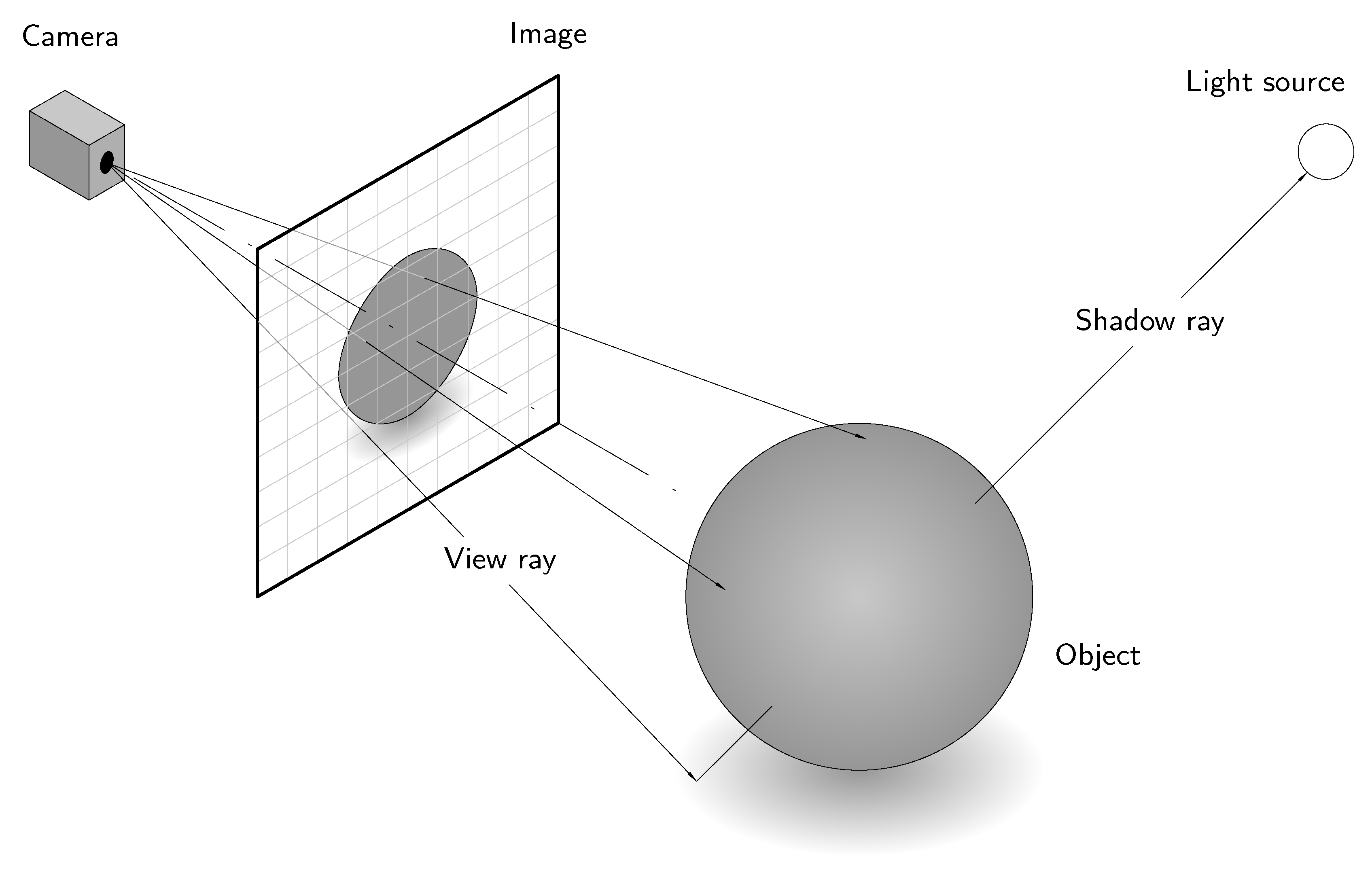
In connection with the algorithms described previously, a related class of methods is often used for the visual representation of primarily three-dimensional scenes. The so-called ray tracing techniques are a frequently used method in the field of computer graphics for the generation of realistic light and shadow effects and thus contribute to a realistic representation of three-dimensional objects, as is the case with rendering, for example. Accordingly, the calculation of the isosurfaces precedes the application of ray tracing, but this method certainly offers added value with regard to the visual representation of simulation results, for instance. The basic idea of ray tracing is to expose the (previously calculated) isosurfaces to artificial light rays from a virtual light source and to observe the course of the light rays in order to determine the lighting conditions in the image; see Figure 10.

Figure 10.
Qualitative illustration of the ray tracing method based on [55].
In the first step, the image is divided into pixels, whereby a ray is generated for each pixel of the image. Here, the ray is described by a parameterized line in Equation (11), which is defined by two points and a scaling factor [55].
This ray then travels from the viewer through the pixel into the respective scene and represents the viewer’s line of sight. The generated rays are of particular importance in this context, as they are used to calculate the light and shadow ratios. The rays are followed as they propagate through the scene and their interaction with the objects in the scene is observed. Here, we are particularly interested in where the ray intersects the corresponding scene. In the event that the ray has crossed an object in the scene, it is then checked whether this point is in shadow. This is done by determining whether the point is illuminated by a light source. If, for example, an obstacle blocks the direct connecting line between the point and the light source, the point is in the shadow. In the event that the point is not in shadow, lighting calculations are subsequently carried out that take into account, among other aspects, the incident ambient light and the effects caused by the irradiation of direct and indirect light resulting from reflections. Other influencing variables in this context are, for example, the surface properties, which take into account the respective color tones and the reflexion coefficients. The stored reflexion coefficients can be used to determine whether the ray hits a reflective surface. If this is the case, a new reflexion ray is generated and the entire process is repeated for this ray. For transparent materials, on the other hand, a refracted ray is generated. The calculated color values for each ray are accumulated to obtain the final color value for the pixel. In the event that reflections or refractions occur, the described process is continued recursively, which means that, for each reflected or refracted ray, the ray tracing process is performed again. The entire process is then repeated for each pixel on the image surface to obtain the final image. As mentioned above, the ray tracing method offers the possibility of displaying realistic scenes. However, this is counteracted by the high level of computational effort.
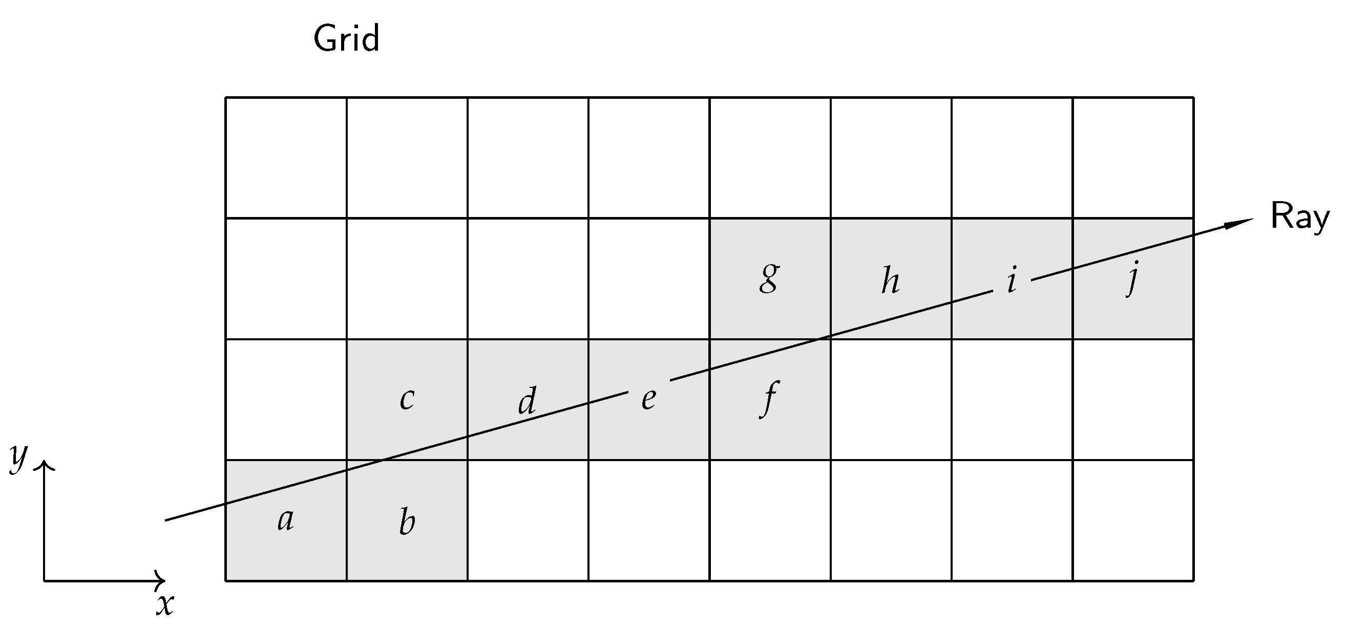
In this context, it can be stated that the technique of ray tracing is the subject of current research work, with the first preliminary work in this field having been carried out by A. Appel [56] and intensified in the 1980s, especially by T. Whitted [57]. At that time, the potential of the method was already recognized, but it was hindered by the intensive computational effort required. For this reason, the initial research work in this field focused on developing approaches to reduce the computational cost. For example, J. Amanatides and A. Woo present, in [58], a simplified method to reduce the computational effort and introduce an incremental transversal algorithm; see Figure 11. The idea is to first identify the voxel in which the ray origin lies and then determine the value at which the ray passes the boundary of the first vertical voxel.
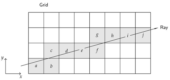
Figure 11.
Grid traversed by a ray based on [58]; ray visits voxels from a to j.
An identical step is performed for the other spatial direction. The minimum of both calculated values then indicates the extent to which it is possible to move along the beam without leaving the voxel.
In their work, the authors S. Parker et al. show how the isosurface of an object can be determined using the ray tracing method on the basis of analytical approaches [59]. The ray under consideration is interpreted as a vector. Each cell is checked to determine whether its data range is bounded by a defined isovalue. If this is the case, an analytical calculation is performed to determine the ray parameter t that defines the intersection point. The entire procedure is then carried out for all cells. To validate the procedure, the authors apply the method developed to the Visible Woman data set [60].
Y. Livnat and C. Hansen present, in [61], a ray tracing method to visualize the polygonal isosurface of the visible part of the isosurface. In the first phase, coarse visibility tests are performed to identify the visible cells. The visible parts of the extracted triangles are then resolved and processed by the graphics hardware.
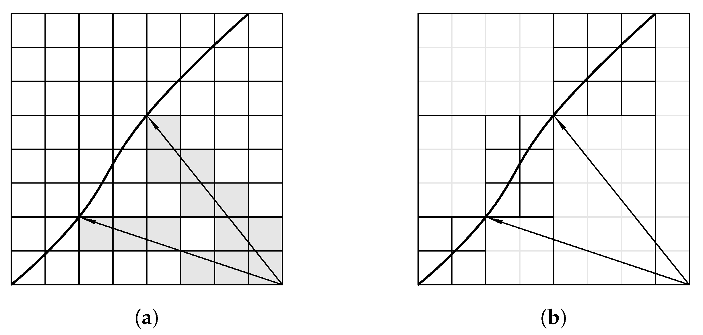
The possible integration of implicit kd-trees ([62], p. 99) for the determination of the isosurface and simultaneous rendering is presented by I. Wald et al. in [63]. Here, Figure 12 illustrates the method.
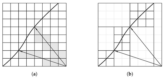
Figure 12.
Application of kd-tress in ray tracing based on [63]: (a) conventional approach, (b) exploiting property of kd-trees to skip large empty regions.
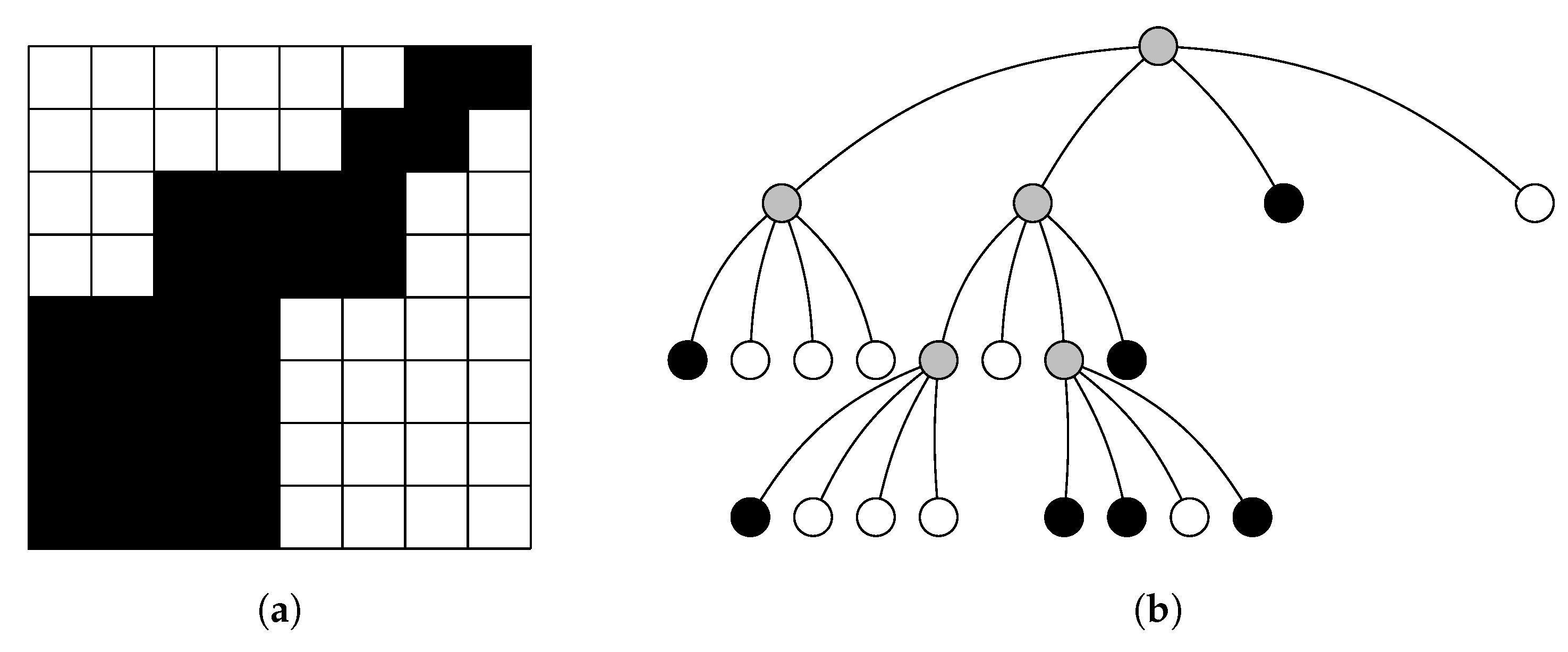
The idea of the approach essentially consists of two parts: on the one hand, a kd-tree contains information about which isosurfaces are contained and a modified transversal algorithm runs through the kd-tree and also implicitly classifies whether the corresponding node contains the defined isovalue. This also allows large empty areas to be skipped more quickly, which is also adressed by N. Morrical et al. in [64]. Therefore, the method presented has the advantage that it requires less memory than conventional methods. An extension of the approach can be found in [65]. Further applications of kd-trees can be found in [1,66,67,68], for example. Another alternative for the efficient handling of large data sets is the use of so-called octree-based, hierarchical data structures. As indicated in their name, octrees describe the recursive decomposition of a space into eight sub-volumes (or four cells in the two-dimensional case). The root of the octree represents the entire volume; see Figure 13.

Figure 13.
Application of octrees based on [69]: (a) active cells in black, (b) corresponding octree.
Research on the use of octree-based approaches can be found in [69,70,71,72]. A. Knoll et al. present, in [73], an approach based on an octree volume format and a traversal method that allows the faster ray tracing of compressed scalar volume data. The method is particularly suitable for large volume data, whereas GPU volume renderers are preferable for smaller volume data, according to the authors. In [74], a further development of the procedure is described.
In [75], authors B. Nelson and R. M. Kirby develop a ray tracing isosurface algorithm for spectral/ element methods, which are higher-order finite element methods. The method can be used to both quantify and minimize the visualization error that occurs. The intersection point between the ray and the isosurface is determined on the basis of analytical methods. The advantage of this method is that the polynomial approximation can be adapted to the true solution as precisely as required. In addition, the convergence speed is higher than with other classical low-order methods, such as marching cubes algorithms.
To process unstructured data sets, P. Rosenthal and L. Linsen present an approach in [76] that is based on the use of partial differential equations (PDE). The advantage of the method is that no resampling of the data or mesh generation is required. The authors use the information regarding the neighborhood relationships to estimate the gradients and mean curvature at each individual sampling point using a four-dimensional least-square fitting approach, as these are necessary for the use of the PDE-based method.
In [77], A. Schollmeyer and B. Froehlich propose a method of determining the isosurface that incorporates a NURBS-based isogeometric analysis. The main aspects of the novel approach include a ray generation scheme that only generates rays that tend to contribute to the subsequent image creation. In addition, there is a method to determine all intersection points of the rays with the curved surface and a solution approach for memory management. In the course of validating the method, the authors find that the approach that they present is both faster and more accurate than GPU-based ray casting approaches. Further research work in the field of ray tracing can be found in [78,79,80]. Table 4 provides a condensed overview of the ray tracing methods described in the literature.
Table 4.
Summary of research work related to ray tracing techniques.
6. Proposed Future Research Activities
The investigation carried out in this paper shows that the assessment of the suitability of the algorithms presented is primarily based on a quantitative analysis in the form of a visual representation of the results. This is mainly the consequence of the original objective for the respective application. Another criterion that is often the subject of evaluation is the computing capacity required, as large volumes of data are usually analyzed. This applies in particular to ray tracing methods.
However, we note that there is no general scheme for the evaluation of the developed algorithms according to a defined standard. We therefore propose, as future research work, to develop and establish a standardized test procedure in order to be able to generate reliable statements regarding the performance of the procedures to be examined with regard to the fulfillment of the task described in Definition 1 and to create a basis for the comparison of the individual procedures. In the field of numerics, the following categories are of particular interest, which we propose as evaluation criteria for isocontouring methods:
- condition;
- stability;
- consistency; and
- convergence.
6.1. Condition
The condition of the problem describes the extent to which the problem oscillates in the event of any perturbations. This is particularly important for so-called inverse problems, where the cause of the problem must be deduced from the effect. This often occurs when calculating inverse matrices, where a variation in the entries of the matrix can have a significant effect on the solution. In this context, one can also speak of ill-posed problems. Various regularization techniques exist to mitigate these effects, such as Tikhonov regularization [81]. However, the extent to which this category needs to be examined in relation to isocontouring methods depends on the method proposed.
6.2. Stability
In contrast to condition, stability refers to the oscillation of the numerical algorithm in the event of possible perturbations, i.e., how sensitively the algorithm reacts to a perturbation in the input parameters. An example of this would be the extent to which the distortion of an originally structured data set affects the quality of the result.
6.3. Consistency
The consistency of the method refers to the actual solution to the original problem. If it is assumed that the analytical solution to a problem is known, the consistency checks the extent to which the algorithm deviates from the analytical solution if the input is exact. An example of this would be the numerical calculation of one-dimensional zeros, whereby the analytically known zero is passed to the procedure in order to subsequently check how large the deviation from the target value (in this case, 0) is.
6.4. Convergence
Convergence is similar to the consistency of the algorithm and examines the extent to which the problem is solved with perturbed input data. In the context of convergence, the speed with which the solution is approximated is of central importance.
Although the above categories allow a standardized examination of the developed methods, they require knowledge of the analytical solution. For this reason, we suggest introducing suitable test functions that have an appropriate degree of complexity and whose analytical solution is known. A possible function for two-dimensional solution sets would be, for example, the simple parabolic function of the form . In this case, a value calculated by the algorithm, which should result in a previously defined function value v, can then be inserted into the analytical form in order to review the quality with which the nominal value was approximated, i.e., is calculated, with being the deviation according to the nominal value. Note that the use of test functions is common practice in the field of nonlinear optimization—for instance, in order to verify the solution quality of developed algorithms. Examples include Himmelblau’s function [82] or the Rosenbrock function [83]. To obtain a statistically reliable statement, a certain number of experiments must also be carried out. Here, it is important to limit the number of parameters to be varied in the experiments to a manageable level. In this context, the authors J. Loeppky et al. propose, in [84], that the number of computer experiments to be carried out should be determined by the relation , where describes the number of parameters to be varied. Subsequent statistical evaluation can then be used to draw conclusions about the quality of the procedure by using the arithmetic mean and the corresponding standard deviation. However, the method that we propose requires that the results obtained by the algorithm are available in a form that is suitable for evaluation in the categories mentioned, such as the generation of point clouds that can be used as raw data.
Key aspects of the proposed method have already been successfully demonstrated in [39] through the systematic comparison of two functions in MATLAB© for isocontouring. The categories considered include the quality of the results achieved, taking into account perturbations in the input data and the computing time required. Test functions were defined in analytical form in advance in order to be able to compare the calculated results with the exact solution in each case. With the help of the procedure, it was thus possible to make quantitative statements with regard to the investigated aspects, in addition to the qualitative presentation of the results.
7. Discussion
The previous sections describing the various methods reveal that they all have specific limitations and are used in certain areas of application. Therefore, the methods are first summarized, compared and discussed. As the methods presented were all developed and implemented in different application areas, the algorithms are first discussed within their method families which finally leads to a cross-method analysis.
7.1. Marching Squares and Marching Cubes Algorithms
Overall, the marching squares and marching cubes algorithms provide a robust method to calculate isovalues within a given data set. The main application of the process is in imaging techniques, such as for medical purposes. The original data are therefore structured as image recordings and divided into pixels. It is not possible to vectorize the algorithm, as the data cubes have to be analyzed individually, which has a significant impact on the overall speed of the algorithms. Since structured data in grid form must be available for the application of the algorithm, transferability is only possible to problems that incorporate exactly these types of data structures. This limits the applicability of the algorithm to predominantly imaging problems. Furthermore, the results of the marching cubes algorithms are mainly tested using visual inspections, or, in some cases, a comparison is carried out with the original marching cubes algorithm of W. E. Lorensen and H. E. Cline.
7.2. Tessellation-Based Algorithms
The tessellation-based algorithms are made up of several different approaches, all of which are based on polygonization or the general use of triangles or tetrahedra. The polygonization algorithms, and the marching tetrahedra algorithm in particular, are based on the fundamental idea of the marching cubes algorithm and therefore originate primarily from the field of medical imaging. However, the methods have also been extended to the generation and triangulation of molecular surfaces, for example. These methods require structured data but often provide topologically more correct surfaces than the marching cubes algorithm. Mesh-based algorithms, on the other hand, originate from a different problem-solving context, where primarily technical problems need to be solved. Structured data are generally not available for these problems, meaning that the algorithms must also provide results with unstructured data. This means that these algorithms could also be used in other areas.
Thus, it can be concluded that the tessellation-based algorithms are primarily used for structured data sets and are only occasionally used for unstructured data sets. The data sets can be two- or three-dimensional. The quality of the various algorithms, if validation is carried out, is predominantly analyzed via a visual inspection. The RooTri() algorithm in [39] is an exception, as it can be used for unstructured data sets and a test routine based on statistically sound methods is performed to evaluate the quality of the algorithm.
7.3. Surface Nets Algorithms
The general concept of the surface nets algorithm is based on the approach of the marching cubes algorithm, whereby cubes are constructed from layered, structured data. The method is therefore preferably used in the field of medical imaging, which provides structured data for evaluation. In addition to medical imaging, the method is also used in computer geometry and offers a simple and effective procedure for the determination of isocontours or isosurfaces. By smoothing the surfaces, the terracing effect can also be significantly reduced. However, the method does not always produce the most accurate or precise surface meshes, especially for complex geometries or strong curvatures. It can also be observed that the quality of the surface nets algorithms is only evaluated by means of visual inspection, while a comparison with the original marching cubes algorithm by W. E. Lorensen and H. E. Cline is only carried out in one case.
7.4. Ray Tracing Algorithms
In the field of computer graphics, such as the visualization of simulation results, ray tracing algorithms offer the possibility of generating realistic light and shadow effects for three-dimensional scenes. However, this leads to great computational effort overall. The method also requires predominantly structured data, although approaches that can also process unstructured data have recently been pursued. It is found that the quality of the ray tracing method is mainly determined by visual inspections. However, due to the overall great computational effort of the method, the resulting computational cost of the algorithms is also a frequently used criterion.
In summary, it can be stated that the methods were all developed from their respective areas of application and therefore require a specific form of data, often structured data. However, this frequently makes it difficult to transfer them to other areas of application that provide different data. Furthermore, the assessment of the algorithm quality largely relies on visual inspection, posing challenges in comparing different method families.
8. Conclusions
This paper provides a comprehensive overview of approaches for the determination of isocontours and isosurfaces from given data sets. Based on the review of existing algorithms for iscontouring, four dominant methods can be identified: marching cubes algorithms, tessellation-based algorithms, surface nets algorithms and ray tracing algorithms. The algorithms have each been developed from specific problem areas; thus, the corresponding solution strategies for isocontouring have also resulted from these contexts. Nevertheless, all algorithms must solve the same task from a mathematical point of view. With regard to their application, it can be seen that the methods are mainly used in the fields of medical imaging, computer graphics and the visualization of simulation results. The preferred areas of application of the algorithms also imply that they have different requirements for the necessary input data. Marching cubes and surface nets algorithms, for example, can only process structured data sets. In contrast, tessellation-based methods and ray tracing algorithms are also able to process unstructured data sets. This is particularly advantageous when using measurement data, as these can be subject to errors due to measurement inaccuracies. Another key finding of the literature review is that there is no standardized scheme for the evaluation of the quality of the algorithms developed. Depending on the use case, different categories are examined, most of which involve a visual inspection of the results. Therefore, a possible scheme for the statistical analysis of the developed algorithms is proposed in this paper.
Author Contributions
Conceptualization, K.J.B., J.P.D. and J.O.; methodology, K.J.B., J.P.D. and J.O.; validation, K.J.B., J.P.D. and J.O.; formal analysis, K.J.B., J.P.D. and J.O.; investigation, K.J.B., J.P.D. and J.O.; resources, K.J.B., J.P.D. and J.O.; data curation, K.J.B., J.P.D. and J.O.; writing—original draft preparation, K.J.B., J.P.D. and J.O.; writing—review and editing, K.J.B., J.P.D. and J.O.; visualization, J.O. All authors have read and agreed to the published version of the manuscript.
Funding
This research did not receive any external funding.
Data Availability Statement
Not applicable.
Acknowledgments
The authors acknowledge support by the KIT-Publication Fund of the Karlsruhe Institute of Technology and would like to thank the reviewers for their detailed reading and helpful remarks to improve the quality of the work.
Conflicts of Interest
The authors declare that they have no known competing financial interests or personal relationships that could have appeared to influence the work reported in this paper.
References
- Livnat, Y.; Shen, H.W.; Johnson, C. A Near Optimal Isosurface Extraction Algorithm Using the Span Space. IEEE Trans. Vis. Comput. Graph. 1996, 2, 73–84. [Google Scholar] [CrossRef]
- Lorensen, W.E.; Cline, H.E. Marching Cubes: A High Resolution 3D Surface Construction Algorithm. SIGGRAPH Comput. Graph. 1987, 21, 163–169. [Google Scholar] [CrossRef]
- Henn, C.; Teschner, M.; Engel, A.; Aebi, U. Real-Time Isocontouring and Texture Mapping Meet New Challenges in Interactive Molecular Graphics Applications. J. Struct. Biol. 1996, 116, 86–92. [Google Scholar] [CrossRef]
- Shirley, P.; Tuchman, A. A Polygonal Approximation to Direct Scalar Volume Rendering. In Proceedings of the 1990 Workshop on Volume Visualization, VVS ’90, San Diego, CA, USA, 10–11 December 1990; pp. 63–70. [Google Scholar] [CrossRef]
- Nielson, G.; Hamann, B. The Asymptotic Decider: Resolving the Ambiguity in Marching Cubes. In Proceedings of the Visualization ’91, San Diego, CA, USA, 22–25 October 1991; pp. 83–91. [Google Scholar] [CrossRef]
- Chernyaev, E.V. Marching Cubes 33: Construction of Topologically Correct Isosurfaces. In Proceedings of the GRAPHICON ’95, St. Petersburg, Russia, 3–7 July 1995. [Google Scholar]
- Natarajan, B.K. On generating topologically consistent isosurfaces from uniform samples. Vis. Comput. 1994, 11, 52–62. [Google Scholar] [CrossRef]
- Wang, X.; Gao, S.; Wang, M.; Duan, Z. A marching cube algorithm based on edge growth. Virtual Real. Intell. Hardw. 2021, 3, 336–349. [Google Scholar] [CrossRef]
- Xu, Z.; Xiao, C.; Xu, X. An improved Marching Cubes algorithm based on edge contraction. In Proceedings of the IEEE 10th International Conference on Signal Processing Proceedings, Beijing, China, 24–28 October 2010; pp. 944–947. [Google Scholar] [CrossRef]
- Nielson, G. Dual marching cubes. In Proceedings of the IEEE Visualization 2004, Austin, TX, USA, 10–15 October 2004; pp. 489–496. [Google Scholar] [CrossRef]
- Gong, S.; Newman, T.S. Dual Marching Squares: Description and analysis. In Proceedings of the 2016 IEEE Southwest Symposium on Image Analysis and Interpretation (SSIAI), Santa Fe, NM, USA, 6–8 March 2016; pp. 53–56. [Google Scholar] [CrossRef]
- Grosso, R.; Zint, D. A parallel dual marching cubes approach to quad only surface reconstruction. Vis. Comput. 2022, 38, 1301–1316. [Google Scholar] [CrossRef]
- Gong, S.; Newman, T.S. A corner feature sensitive marching squares. In Proceedings of the 2013 Proceedings of IEEE Southeastcon, Jacksonville, FL, USA, 4–7 April 2013; pp. 1–6. [Google Scholar] [CrossRef]
- Gong, S.; Newman, T.S. Isocontouring with Sharp Corner Features. Mach. Graph. Vis. 2018, 27, 21–46. [Google Scholar] [CrossRef]
- Raman, S.; Wenger, R. Quality Isosurface Mesh Generation Using an Extended Marching Cubes Lookup Table. Comput. Graph. Forum 2008, 27, 791–798. [Google Scholar] [CrossRef]
- Custodio, L.; Pesco, S.; Silva, C. An extended triangulation to the Marching Cubes 33 algorithm. J. Braz. Comput. Soc. 2019, 25, 6. [Google Scholar] [CrossRef]
- Gong, S.; Newman, T.S. Fine feature sensitive marching squares. IET Image Process. 2017, 11, 796–802. [Google Scholar] [CrossRef]
- He, Y.; Mirzargar, M.; Hudson, S.; Kirby, R.M.; Whitaker, R.T. An Uncertainty Visualization Technique Using Possibility Theory: Possibilistic Marching Cubes. Int. J. Uncertain. Quantif. 2015, 5, 433–451. [Google Scholar] [CrossRef]
- Newman, T.S.; Yi, H. A survey of the marching cubes algorithm. Comput. Graph. 2006, 30, 854–879. [Google Scholar] [CrossRef]
- Payne, B.A.; Toga, A.W. Surface mapping brain function on 3D models. IEEE Comput. Graph. Appl. 1990, 10, 33–41. [Google Scholar] [CrossRef]
- Bloomenthal, J. An Implicit Surface Polygonizer. In Graphics Gems IV; Academic Press Professional, Inc.: Cambridge, MA, USA, 1994; pp. 324–349. [Google Scholar] [CrossRef]
- Guéziec, A.; Hummel, R. The wrapper algorithm for surface extraction in volumetric data. In Proceedings of the Symposium on Applications of Computer Vision in Medical Image Processing, Palo Alto, CA, USA, 21–23 March 1994; pp. 227–231. [Google Scholar]
- Guéziec, A.; Hummel, R. The wrapper algorithm: Surface extraction and simplification. In Proceedings of the IEEE Workshop on Biomedical Image Analysis, Seattle, WA, USA, 24–25 June 1994; pp. 204–213. [Google Scholar] [CrossRef]
- Guéziec, A.; Hummel, R. Exploiting triangulated surface extraction using tetrahedral decomposition. IEEE Trans. Vis. Comput. Graph. 1995, 1, 328–342. [Google Scholar] [CrossRef]
- Zhou, Y.; Chen, W.; Tang, Z. An elaborate ambiguity detection method for constructing isosurfaces within tetrahedral meshes. Comput. Graph. 1995, 19, 355–364. [Google Scholar] [CrossRef]
- Nielson, G.M.; Franke, R. Computing the separating surface for segmented data. In Proceedings of the Visualization ’97 (Cat. No. 97CB36155), Phoenix, AZ, USA, 24 October 1997; pp. 229–233. [Google Scholar] [CrossRef]
- Bonnell, K.S.; Schikore, D.R.; Joy, K.I.; Duchaineau, M.; Hamann, B. Constructing material interfaces from data sets with volume-fraction information. In Proceedings of the Visualization 2000. VIS 2000 (Cat. No.00CH37145), Salt Lake City, UT, USA, 8–13 October 2000; pp. 367–372. [Google Scholar] [CrossRef]
- Chan, S.L.; Purisima, E.O. A new tetrahedral tesselation scheme for isosurface generation. Comput. Graph. 1998, 22, 83–90. [Google Scholar] [CrossRef]
- Chan, S.L.; Purisima, E.O. Molecular surface generation using marching tetrahedra. J. Comput. Chem. 1998, 19, 1268–1277. [Google Scholar] [CrossRef]
- Lu, T.; Chen, F. Quantitative analysis of molecular surface based on improved Marching Tetrahedra algorithm. J. Mol. Graph. Model. 2012, 38, 314–323. [Google Scholar] [CrossRef] [PubMed]
- Treece, G.M.; Prager, R.W.; Gee, A.H. Regularised marching tetrahedra: Improved iso-surface extraction. Comput. Graph. 1999, 23, 583–598. [Google Scholar] [CrossRef]
- Cong, A.; Liu, Y.; Kumar, D.; Cong, W.; Wang, G. Geometrical modeling using multiregional marching tetrahedra for bioluminescence tomography. In Proceedings of the Medical Imaging 2005: Visualization, Image-Guided Procedures, and Display, San Diego, CA, USA, 12–17 February 2005; Galloway, R.L., Jr.;Cleary, K.R., Eds.; International Society for Optics and Photonics, SPIE: Bellingham, WA, USA, 2005; Voumel 5744, pp. 756–763. [Google Scholar] [CrossRef]
- Nielson, G.M. Dual Marching Tetrahedra: Contouring in the Tetrahedronal Environment. In Proceedings of the 4th International Symposium on Advances in Visual Computing, ISVC ’08, Las Vegas, NV, USA, 1–3 December 2008; pp. 183–194. [Google Scholar] [CrossRef]
- d’Otreppe, V.; Boman, R.; Ponthot, J.P. Generating smooth surface meshes from multi-region medical images. Int. J. Numer. Methods Biomed. Eng. 2012, 28, 642–660. [Google Scholar] [CrossRef] [PubMed]
- Shen, T.; Gao, J.; Yin, K.; Liu, M.Y.; Fidler, S. Deep marching tetrahedra: A hybrid representation for high-resolution 3d shape synthesis. Adv. Neural Inf. Process. Syst. 2021, 34, 6087–6101. [Google Scholar] [CrossRef]
- Guo, J.; Wang, X.; Wang, J.; Dai, X.; Wu, L.; Li, C.; Li, F.; Liu, S.; Jessell, M.W. Three-dimensional geological modeling and spatial analysis from geotechnical borehole data using an implicit surface and marching tetrahedra algorithm. Eng. Geol. 2021, 284, 106047. [Google Scholar] [CrossRef]
- Sun, H.; Zhong, D.; Wu, Z.; Wang, L. Multi-labeled Regularized Marching Tetrahedra Method for Implicit Geological Modeling. Math. Geosci. 2023, 1–30. [Google Scholar] [CrossRef]
- Bajaj, C.L.; Pascucci, V.; Schikore, D.R. Fast isocontouring for improved interactivity. In Proceedings of the 1996 Symposium on Volume Visualization, San Francisco, CA, USA, 29 October 1996; pp. 39–46. [Google Scholar] [CrossRef]
- Oellerich, J.; Büscher, K.J.; Degel, J.P. RooTri: A Simple and Robust Function to Approximate the Intersection Points of a 3D Scalar Field with an Arbitrarily Oriented Plane in MATLAB. Algorithms 2023, 16, 409. [Google Scholar] [CrossRef]
- Lewiner, T.; Velho, L.; Lopes, H.; Mello, V. Hierarchical Isocontours Extraction and Compression. In Proceedings of the Computer Graphics and Image Processing, XVII Brazilian Symposium, SIBGRAPI ’04, Curitiba, Brazil, 20 October 2004; pp. 234–241. [Google Scholar] [CrossRef]
- Lewiner, T.; Lopes, H.; Velho, L.; Mello, V. Extraction and compression of hierarchical isocontours from image data. Comput. Med. Imaging Graph. 2006, 30, 231–242. [Google Scholar] [CrossRef] [PubMed]
- Schlei, B.R. A new computational framework for 2D shape-enclosing contours. Image Vis. Comput. 2009, 27, 637–647. [Google Scholar] [CrossRef]
- Glander, T.; Trapp, M.; Döllner, J. 3D Isocontours Real-time Generation and Visualization of 3D Stepped Terrain Models. In Eurographics 2010—Short Papers; Lensch, H.P.A., Seipel, S., Eds.; The Eurographics Association: Eindhoven, The Netherlands, 2010. [Google Scholar] [CrossRef]
- Panagiotakis, C.; Kokinou, E. Unsupervised detection of topographic highs with arbitrary basal shapes based on volume evolution of isocontours. Comput. Geosci. 2017, 102, 22–33. [Google Scholar] [CrossRef]
- Gibson, S.F.F. Constrained elastic surface nets: Generating smooth surfaces from binary segmented data. In Proceedings of the Medical Image Computing and Computer-Assisted Intervention—MICCAI’98, Cambridge, MA, USA, 11–13 October 1998; Wells, W.M., Colchester, A., Delp, S., Eds.; Springer: Berlin/Heidelberg, Germany, 1998; pp. 888–898. [Google Scholar] [CrossRef]
- Gibson, S.F. Surface Net Smoothing for Surface Representation from Binary Sampled Data. US Patent 6,084,593, 14 May 1998. [Google Scholar]
- Gibson, S.F.F. Using distance maps for accurate surface representation in sampled volumes. In Proceedings of the IEEE Symposium on Volume Visualization (Cat. No.989EX300), Research Triangle Park, NC, USA, 19–20 October 1998; pp. 23–30. [Google Scholar] [CrossRef]
- Leventon, M.E.; Gibson, S.F.F. Model Generation from Multiple Volumes Using Constrained Elastic SurfaceNets. In Proceedings of the Information Processing in Medical Imaging, Visegrad, Hungary, 28 June–2 July 1999; Kuba, A., Šáamal, M., Todd-Pokropek, A., Eds.; Springer: Berlin/Heidelberg, Germany, 1999; pp. 388–393. [Google Scholar] [CrossRef]
- de Bruin, P.W.; Vos, F.M.; Post, F.H.; Frisken-Gibson, S.F.; Vossepoel, A.M. Improving Triangle Mesh Quality with SurfaceNets. In Proceedings of the Medical Image Computing and Computer-Assisted Intervention—MICCAI 2000, Pittsburgh, PA, USA, 11–14 October 2000; Delp, S.L., DiGoia, A.M., Jaramaz, B., Eds.; Springer: Berlin/Heidelberg, Germany, 2000; pp. 804–813. [Google Scholar] [CrossRef]
- Baxter, J.S.H.; Peters, T.M.; Chen, E.C.S. A unified framework for voxel classification and triangulation. In Proceedings of the Medical Imaging 2011: Visualization, Image-Guided Procedures, and Modeling, Orlando, FL, USA, 12–17 February 2011; Wong, K.H., Holmes, D.R., III, Eds.; International Society for Optics and Photonics, SPIE: Bellingham, WA, USA, 2011; Volume 7964, p. 796436. [Google Scholar] [CrossRef]
- Frisken, S.F. SurfaceNets for Multi-Label Segmentations with Preservation of Sharp Boundaries. J. Comput. Graph. Tech. (JCGT) 2022, 11, 34–54. [Google Scholar]
- Frisken, S.F.; Perry, R.N.; Rockwood, A.P.; Jones, T.R. Adaptively Sampled Distance Fields: A General Representation of Shape for Computer Graphics. In Proceedings of the 27th Annual Conference on Computer Graphics and Interactive Techniques, SIGGRAPH ’00, New Orleans, LA, USA, 23–28 July 2000; pp. 249–254. [Google Scholar] [CrossRef]
- Perry, R.N.; Frisken, S.F. Kizamu: A System for Sculpting Digital Characters. In Proceedings of the 28th Annual Conference on Computer Graphics and Interactive Techniques, SIGGRAPH ’01, Los Angeles, CA, USA, 12–17 August 2001; pp. 47–56. [Google Scholar] [CrossRef]
- Bertram, M.; Reis, G.; van Lengen, R.H.; Köhn, S.; Hagen, H. Non-Manifold Mesh Extraction from Time-Varying Segmented Volumes Used for Modeling a Human Heart. In Proceedings of the Seventh Joint Eurographics/IEEE VGTC Conference on Visualization, EUROVIS’05, Leeds, UK, 1–3 June 2005; pp. 199–206. [Google Scholar]
- Haines, E.; Akenine-Möller, T. Ray Tracing Gems: High-Quality and Real-Time Rendering with DXR and Other APIs; Apress: New York, NY, USA, 2019. [Google Scholar] [CrossRef]
- Appel, A. Some Techniques for Shading Machine Renderings of Solids. In Proceedings of the Spring Joint Computer Conference, AFIPS ’68 (Spring), New York, NY, USA, April 30–May 2 1968; pp. 37–45. [Google Scholar] [CrossRef]
- Whitted, T. An Improved Illumination Model for Shaded Display. Commun. ACM 1980, 23, 343–349. [Google Scholar] [CrossRef]
- Amanatides, J.; Woo, A. A Fast Voxel Traversal Algorithm for Ray Tracing; EG 1987—Technical Papers; Eurographics Association: Eindhoven, The Netherlands, 1987. [Google Scholar] [CrossRef]
- Parker, S.; Shirley, P.; Livnat, Y.; Hansen, C.; Sloan, P.P. Interactive Ray Tracing for Isosurface Rendering. In Proceedings of the Visualization ’98 (Cat. No.98CB36276), Research Triangle Park, NC, USA, 18–23 October 1998; pp. 233–238. [Google Scholar] [CrossRef]
- Waldby, C. The Visible Human Project: Informatic Bodies and Posthuman Medicine; Routledge: Oxfordshire, UK, 2000. [Google Scholar]
- Livnat, Y.; Hansen, C. View Dependent Isosurface Extraction. In Proceedings of the Visualization ’98 (Cat. No.98CB36276), Research Triangle Park, NC, USA, 18–23 October 1998; pp. 175–180. [Google Scholar] [CrossRef]
- de Berg, M.; Cheong, O.; Kreveld, M.; Overmars, M. Computational Geometry, 3rd ed.; Springer: Berlin/Heidelberg, Germany, 2008. [Google Scholar] [CrossRef]
- Wald, I.; Friedrich, H.; Marmitt, G.; Slusallek, P.; Seidel, H.P. Faster Isosurface Ray Tracing Using Implicit KD-Trees. IEEE Trans. Vis. Comput. Graph. 2005, 11, 562–572. [Google Scholar] [CrossRef]
- Morrical, N.; Usher, W.; Wald, I.; Pascucci, V. Efficient Space Skipping and Adaptive Sampling of Unstructured Volumes Using Hardware Accelerated Ray Tracing. In Proceedings of the 2019 IEEE Visualization Conference (VIS), Vancouver, BC, Canada, 20–25 October 2019; pp. 256–260. [Google Scholar] [CrossRef]
- Wald, I.; Friedrich, H.; Knoll, A.; Hansen, C.D. Interactive Isosurface Ray Tracing of Time-Varying Tetrahedral Volumes. IEEE Trans. Vis. Comput. Graph. 2007, 13, 1727–1734. [Google Scholar] [CrossRef] [PubMed]
- Hughes, D.M.; Lim, I.S. Kd-Jump: A Path-Preserving Stackless Traversal for Faster Isosurface Raytracing on GPUs. IEEE Trans. Vis. Comput. Graph. 2009, 15, 1555–1562. [Google Scholar] [CrossRef]
- Wald, I.; Knoll, A.; Johnson, G.P.; Usher, W.; Pascucci, V.; Papka, M.E. CPU ray tracing large particle data with balanced P-k-d trees. In Proceedings of the 2015 IEEE Scientific Visualization Conference (SciVis), Chicago, IL, USA, 25–30 October 2015; pp. 57–64. [Google Scholar] [CrossRef]
- Li, F.; Su, Y. Stackless KD-Tree Traversal For Ray Tracing. In Proceedings of the 2021 2nd International Conference on Electronics, Communications and Information Technology (CECIT), Sanya, China, 27–29 December 2021; pp. 1168–1172. [Google Scholar] [CrossRef]
- Shi, Q.; JaJa, J. Isosurface Extraction and Spatial Filtering using Persistent Octree (POT). IEEE Trans. Vis. Comput. Graph. 2006, 12, 1283–1290. [Google Scholar] [CrossRef] [PubMed]
- Wilhelms, J.; Van Gelder, A. Octrees for Faster Isosurface Generation. ACM Trans. Graph. 1992, 11, 201–227. [Google Scholar] [CrossRef]
- Ju, T.; Losasso, F.; Schaefer, S.; Warren, J. Dual Contouring of Hermite Data. ACM Trans. Graph. 2002, 21, 339–346. [Google Scholar] [CrossRef]
- Wang, C.; Chiang, Y.J. Isosurface Extraction and View-Dependent Filtering from Time-Varying Fields Using Persistent Time-Octree (PTOT). IEEE Trans. Vis. Comput. Graph. 2009, 15, 1367–1374. [Google Scholar] [CrossRef]
- Knoll, A.M.; Wald, I.; Parker, S.; Hansen, C. Interactive Isosurface Ray Tracing of Large Octree Volumes. In Proceedings of the 2006 IEEE Symposium on Interactive Ray Tracing, Salt Lake City, UT, USA, 18–20 September 2006; pp. 115–124. [Google Scholar] [CrossRef]
- Knoll, A.M.; Wald, I.; Hansen, C.D. Coherent multiresolution isosurface ray tracing. Vis. Comput. 2009, 25, 209–225. [Google Scholar] [CrossRef]
- Nelson, B.; Kirby, R. Ray-Tracing Polymorphic Multidomain Spectral/hp Elements for Isosurface Rendering. IEEE Trans. Vis. Comput. Graph. 2006, 12, 114–125. [Google Scholar] [CrossRef]
- Rosenthal, P.; Linsen, L. Smooth Surface Extraction from Unstructured Point-based Volume Data Using PDEs. IEEE Trans. Vis. Comput. Graph. 2008, 14, 1531–1546. [Google Scholar] [CrossRef]
- Schollmeyer, A.; Froehlich, B. Direct Isosurface Ray Casting of NURBS-Based Isogeometric Analysis. IEEE Trans. Vis. Comput. Graph. 2014, 20, 1227–1240. [Google Scholar] [CrossRef]
- Wang, F.; Wald, I.; Wu, Q.; Usher, W.; Johnson, C.R. CPU Isosurface Ray Tracing of Adaptive Mesh Refinement Data. IEEE Trans. Vis. Comput. Graph. 2019, 25, 1142–1151. [Google Scholar] [CrossRef]
- McGraw, T. High-quality real-time raycasting and raytracing of streamtubes with sparse voxel octrees. In Proceedings of the 2020 IEEE Visualization Conference (VIS), Salt Lake City, UT, USA, 25–30 October 2020; pp. 21–25. [Google Scholar] [CrossRef]
- Usher, W.; Dyken, L.; Kumar, S. Speculative Progressive Raycasting for Memory Constrained Isosurface Visualization of Massive Volumes. In Proceedings of the 2023 IEEE 13th Symposium on Large Data Analysis and Visualization (LDAV), Melbourne, Australia, 23 October 2023; pp. 1–11. [Google Scholar] [CrossRef]
- Theu, L.T.; Quang-Huy, T.; Duc-Tan, T.; Sharma, B.; Chowdhury, S.; Chandran, K.; Gurusamy, S. Tikhonov Regularization and Perturbation-Level Tuning for the CNM in Pharmacokinetics. IEEE Access 2023, 11, 30057–30068. [Google Scholar] [CrossRef]
- Naresh Babu, A.; Ramana, T.; Sivanagaraju, S. Analysis of optimal power flow problem based on two stage initialization algorithm. Int. J. Electr. Power Energy Syst. 2014, 55, 91–99. [Google Scholar] [CrossRef]
- Shang, Y.W.; Qiu, Y.H. A Note on the Extended Rosenbrock Function. Evol. Comput. 2006, 14, 119–126. [Google Scholar] [CrossRef] [PubMed]
- Loeppky, J.; Sacks, J.; Welch, W. Choosing the Sample Size of a Computer Experiment: A Practical Guide. Technometrics 2009, 51, 366–376. [Google Scholar] [CrossRef]
Disclaimer/Publisher’s Note: The statements, opinions and data contained in all publications are solely those of the individual author(s) and contributor(s) and not of MDPI and/or the editor(s). MDPI and/or the editor(s) disclaim responsibility for any injury to people or property resulting from any ideas, methods, instructions or products referred to in the content. |
© 2024 by the authors. Licensee MDPI, Basel, Switzerland. This article is an open access article distributed under the terms and conditions of the Creative Commons Attribution (CC BY) license (https://creativecommons.org/licenses/by/4.0/).