Fractional-Order Fuzzy PID Controller with Evolutionary Computation for an Effective Synchronized Gantry System

Abstract

Gantry-type dual-axis platforms can be used to move heavy loads or perform precision CNC work. Such gantry systems drive a single axis with two linear motors, and under heavy loads, a high driving force is required. This can generate a pulling force between the drive shafts in the coupling mechanism. In these situations, when a synchronization error becomes too large, mechanisms can become deformed or damaged, leading to damaged equipment, or in industrial settings, an additional power consumption. Effectively and accurately acquiring the synchronized movement of the platform is important to reduce energy consumption and optimize the system. In this study, a fractional-order fuzzy PID controller (FOFPID) using Oustaloup’s recursive filter is used to control a synchronous X–Y gantry-type platform. The optimized controller parameters are obtained by the measurement of control errors in a simulated environment. Four optimization methods are tested and compared: particle swarm optimization, invasive weed optimization, a gray wolf optimizer, and biogeography-based optimization. The systems were tested and compared in order to optimize the control parameters. Each of the four algorithms is simulated on four contour shapes: a circle, bow, heart, and star. The simulations and control scheme of the experiments are implemented using MATLAB, and the reference paths were planned using non-uniform rational B-splines (NURBS). After running the simulations to determine the optimal control parameters, each set of acquired control parameters is also tested and compared in the experiments and the results are recorded. Both the simulations and experiments show good results, and the tracking of the X–Y platform showed improved performance. Two performance indices are used to determine and validate the relative performance of the models and results.

1. Introduction

Biaxial gantry systems are often found in industrial settings because of their high-speed and high-precision planar motions. Applications include CNC machines, automotive assembly lines, material handling, surface chip mounters, and positioning stages. To provide accurate Cartesian movement information to a multiple-axis configuration, the control stage must be managed in a synchronous manner, especially when carrying heavy loads. Conventional control methods use independent axis control, regardless of the other axes. Synchronous errors cannot be reduced effectively through independent axis control, and this leads to decreased precision in use. Design of a servo control system with synchronous motion techniques [1,2,3,4] is critical for high-precision gantry systems, especially where heavy loads could lead to process safety issues or damage to equipment.

Parallel synchronous control schemes are often driven by two linear motors. Without any mechanical transmission, such as lead screws or gears, the payload can be directly driven. The design in this paper uses a permanent magnet linear synchronous motor (PMLSM) [5] for its compact structure, rapid response, and high force density. Several other approaches to the multi-axis de-synchronization problem have been proposed, such as a master–slave motion control arrangement and cross-coupled controls. In [6], the authors applied a nonlinear feedback control scheme to control the PMLSM position, and overcome inherent nonlinear functions and parametric uncertainties. In [7], a synchronous control was developed on a platform with only one axis, which is actuated by servo motors and dual parallel ball screws. In addition, an identification method was proposed to build a coupled system model. The cross-coupled synchronous control method [8,9] reduced the contouring error in the gantry system. An optimized cross-coupled synchronizing control [8] was proposed to improve synchronization accuracy in dual-feed drives. The performance index includes the synchronous error, which is to be minimized. A cross-coupled synchronous control system was also combined with a complementary sliding mode control [9], to simultaneously converge position tracking and synchronous errors for the gantry position stages with uncertainties. In this study, the authors designed a PID control scheme for an X–Y-type gantry. Since a conventional PID control cannot overcome problems associated with speed changes, load disturbances, and steady-state errors, a fractional-order fuzzy PID (FOFPID) is incorporated for more flexible parameter tuning than that of integer order.

In recent years, fractional order differentiation and integration have become more commonly used in control design [10,11,12,13]. Since the calculus orders are not necessarily to be integers, the dynamic models can be described more adequately. Also, a controller with fractional orders is often more suitable than one using integer orders. A parameter tuning approach for fractional order PD controllers was proposed [14] for a class of second-order systems. This method can increase the robustness by fulfilling the given gain phase margin and crossover frequency. A temperature control with a digital fractional order controller has been demonstrated [15]. Furthermore, the practical application and improvement of PID controllers using fractional order have also been shown [16,17,18]. Another fractional-order fuzzy PID controller design [19] considered tuning the orders in the fuzzy controller, and then used a genetic algorithm to optimize the controller by minimizing error indices.

Although fractional order differ-integrations make the controller adapt to the plant more adequately, tuning the parameters becomes difficult. To improve the effectiveness of the controller design, several optimization algorithms have been used to adjust the parameters, such as particle swarm optimization (PSO) [20], invasive weed optimization (IWO) [21], gray wolf optimization (GWO) [22], biogeography-based optimization (BBO) [23], and genetic algorithms (GAs). In [13,24], the PSO algorithm was used for the adjustment of the fractional order PID controller parameters. The results showed the parameters given by the PSO led to a precise and strong anti-disturbance control. Another work used a modified firefly algorithm (MFA)–PSO-based fractional order PID controller [25] for an effective torque and speed regulation strategy for a BLDC motor. Other optimization algorithms, such as the IWO [26] and GWO [27], were also applied to fractional order controllers to improve their performance.

In this research, the fractional order fuzzy controller is implemented in a synchronized gantry-type X–Y platform. Several optimization algorithms, namely PSO, IWO, BBO, and GWO, are integrated with the FOFPID for precision trajectory tracking control, and their relative performances are compared. The integral of the time-weighted absolute error (ITAE) is an index for the optimization of the controller parameters. Two PMLSMs set up in parallel on the Y-axis rails move a beam simultaneously, while another PMLSM moves the head set up on the beam along the X-axis. A MATLAB system ID toolbox is used to find the parameters of the PMLSM transfer functions. The simulation and experimental results for the different reference contours are demonstrated to reveal the effectiveness of the proposed controller, with improved tracking performance.

This paper is organized as follows: Section 2 presents the system dynamics and model identification. Section 3 describes the fractional-order fuzzy PID controller. The PSO optimization algorithm used in this work is introduced in Section 4. The simulation and experimental results are demonstrated in Section 5, and Section 6 presents the conclusions drawn from the results.

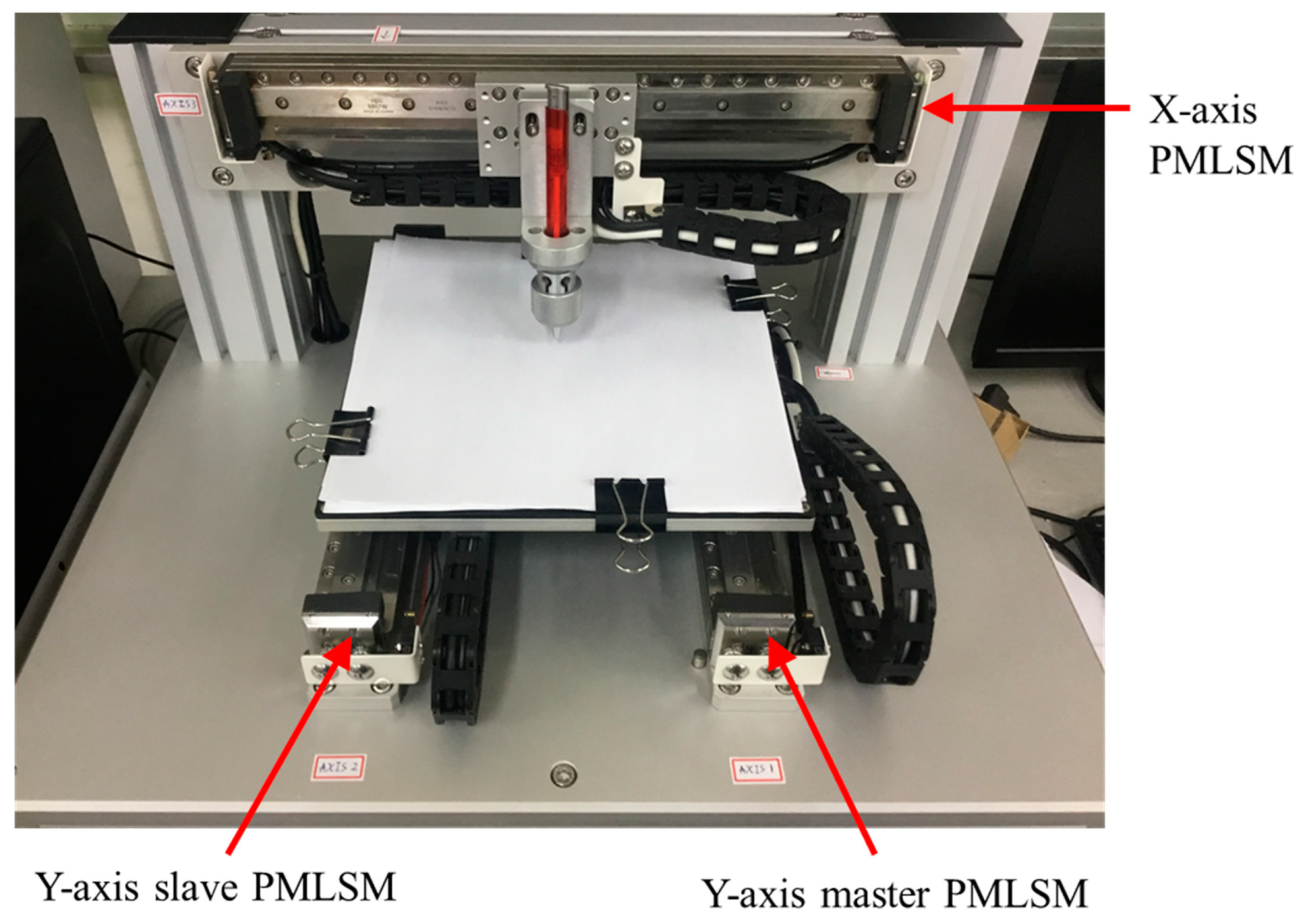
2. System Model and Identification

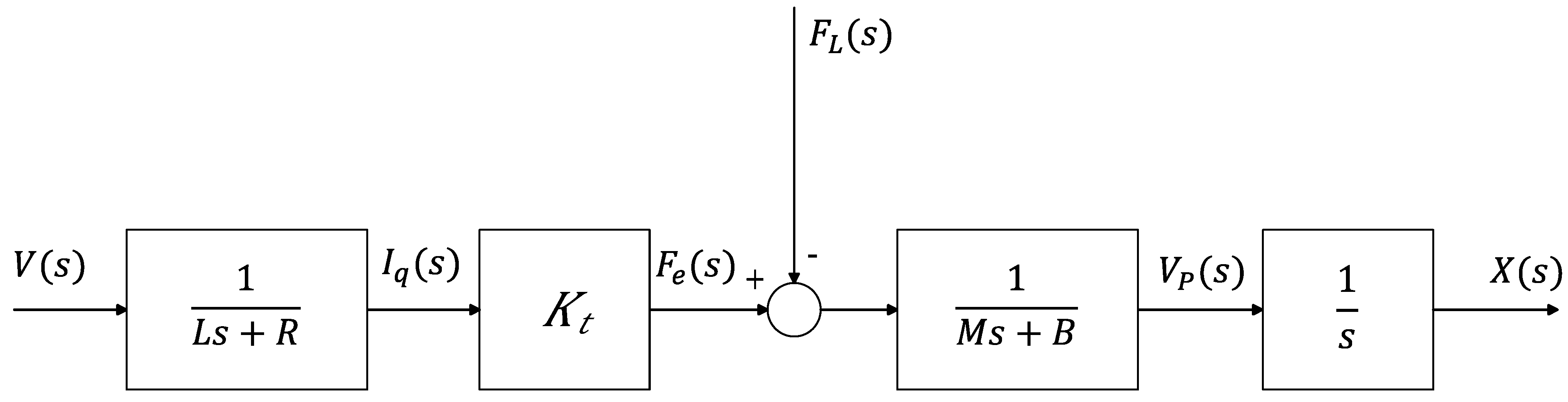
2.1. PMLSM Model

The PMLSMs are used as the actuators in the gantry system and the mathematical model is derived below. The dynamic model [2] in the d–q reference frame is represented by

$$\begin{array}{c}{v}_d=R{i}_d+L_d\frac{d{i}_d}{dt}-\frac{\pi }{\tau }{v}_P{L}_d{i}_q\\ v_q=R{i}_q+L_q\frac{d{i}_q}{dt}+\frac{\pi }{\tau }{v}_P{L}_q{i}_d+\sqrt{\frac{2}{3}}\frac{\pi }{\tau }{\lambda }_{\max }{v}_P\end{array}$$

(1)

where $v_d$ and $v_q$ denote the d-axis and q-axis voltages, $L_d$ and $L_q$ are the d-axis and q-axis inductances, $i_q$ and $i_d$ are the q-axis and d-axis currents, respectively, $\tau$ is the pole pitch, $v_P$ and R are the velocity and resistance of the mover, and ${\lambda }_{\max }$ denotes the maximum of sinusoidal flux linkage. By (1), the derivative of these currents can be obtained as

$$\left[\begin{array}{c}\frac{d{i}_d}{dt}\\ \frac{d{i}_q}{dt}\end{array}\right]=\left[\begin{array}{cc}-\frac{R}{L_d}& -\frac{\pi }{\tau }{v}_P\frac{L_q}{L_d}\\ -\frac{\pi }{\tau }{v}_P\frac{L_d}{L_q}& -\frac{R}{L_q}\end{array}\right]\left[\begin{array}{c}{i}_d\\ i_q\end{array}\right]+\left[\begin{array}{c}\frac{v_d}{L_d}\\ \frac{1}{L_q}\left(v_q-\sqrt{\frac{2}{3}}\frac{\pi }{\tau }{\lambda }_{\max }{v}_P\right)\end{array}\right]$$

(2)

The dynamic equation of the mechanical part is expressed as

$$F_e=M{\dot{v}}_P+B{v}_P+F_L=M\ddot{x}+B\dot{x}+F_L$$

(3)

where M, B, and x are the mass, viscous friction coefficient, and displacement of the stage, respectively, $F_L$ denotes the external loading, and $F_e$ represents the electromagnetic force, which is given by

$$F_e=\frac{3\pi }{2\tau }\left[\left(L_d-L_q\right)i_d{i}_q+{\lambda }_{\max }{i}_q\right]$$

(4)

Since the PMLSM exhibits a uniform air gap on the stator surface, the condition $L_d=L_q=L$ can be assumed and reduces (4) to

$$F_e=\frac{3\pi }{2\tau }{\lambda }_{\max }{i}_q=k_t{i}_q$$

(5)

where $k_t=\frac{3\pi }{2\tau }{\lambda }_{\max }$ is the force constant. Let $v_{dr} \mathrm{and} v_{qr}$ be the d- and q-axis voltage commands and remove the coupled terms, then the derivative of the currents shown in (2) can be rewritten:

$$\left[\begin{array}{c}\frac{d{i}_d}{dt}\\ \frac{d{i}_q}{dt}\end{array}\right]=-\frac{R}{L}\left[\begin{array}{c}{i}_d\\ i_q\end{array}\right]+\frac{1}{L}\left[\begin{array}{c}{v}_{dr}\\ v_{qr}\end{array}\right]$$

(6)

From (5), the q-axis current $i_q$ produces the motor driving force $F_e$. Integrating (3), (5), and (6), and then applying a Laplace transform, provides the transfer function from the voltage command $V\left(s\right)$ to the displacement $X\left(s\right)$:

$$\frac{X\left(s\right)}{V\left(s\right)}=\frac{K_t}{ML{s}^3+(MR+BL)s^2+BRs}$$

(7)

Figure 1 shows the model block diagram of the PMLSM system.

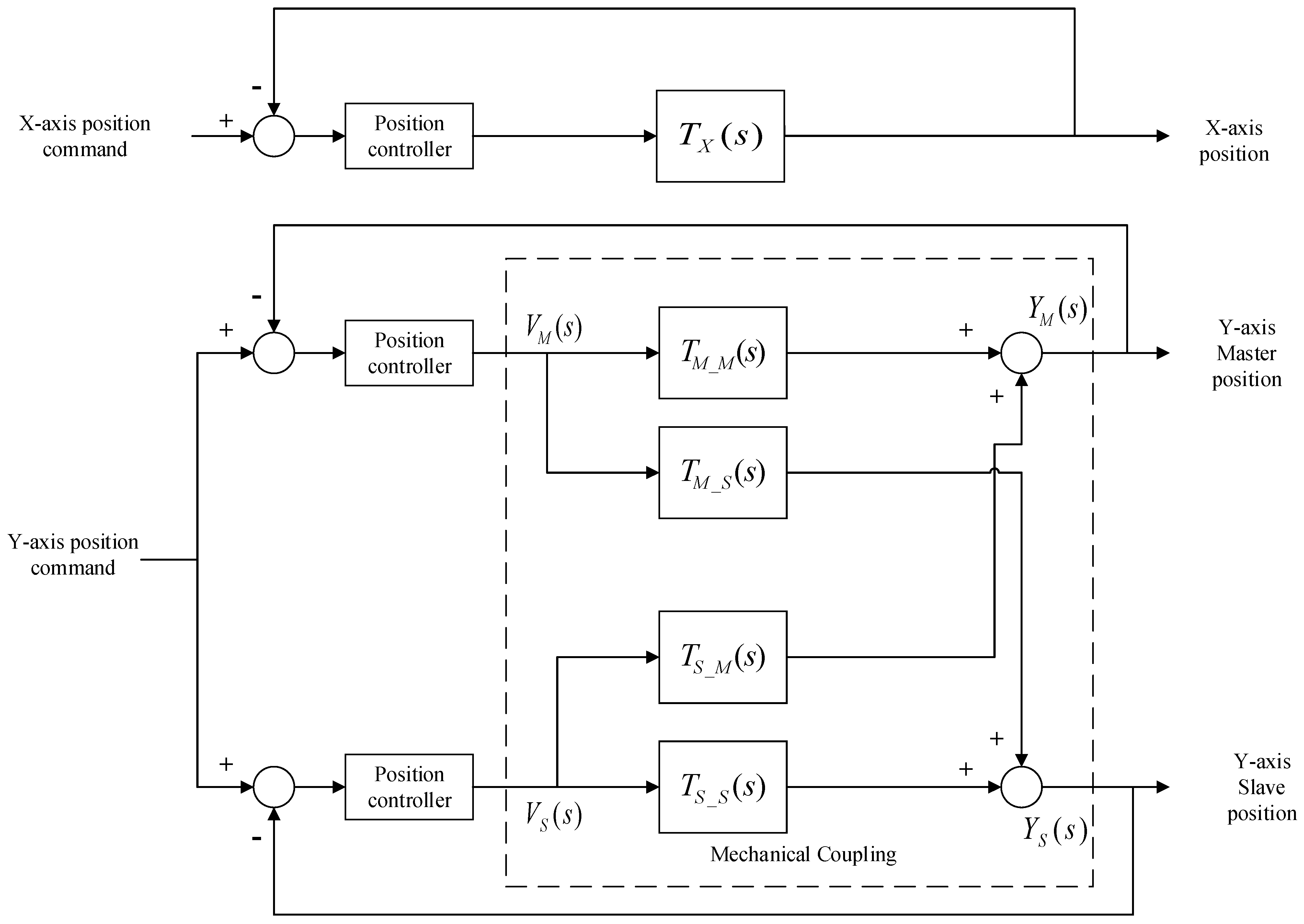
2.2. Mechanical Coupling Model and System Identification

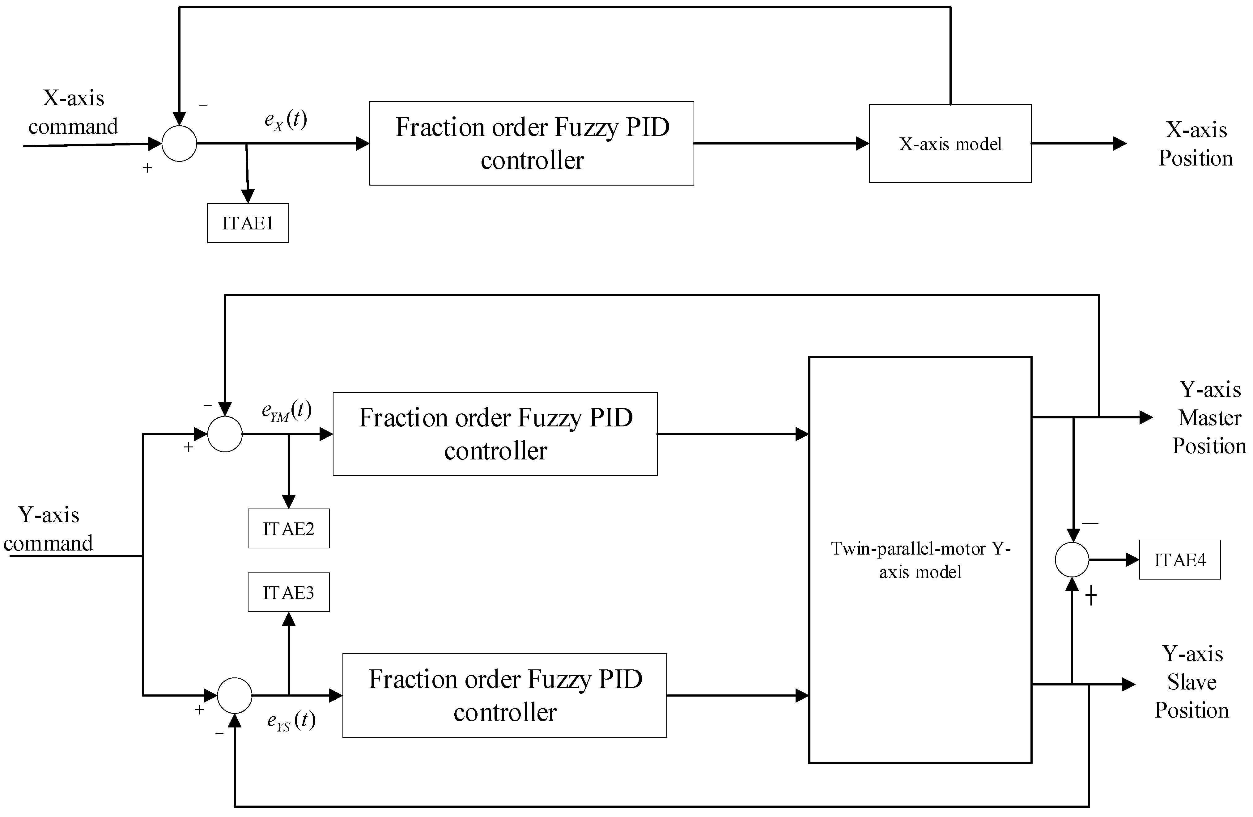
A linear motor is set up on the X-axis of the gantry platform, while the Y-axis consists of two parallel linear motors. Thus, mechanical coupling is inevitable. The displacements on the X- and Y-axis are feedbacked by optical encoders. Figure 2 shows the experimental setup of the gantry system, and the block diagram of the gantry platform is shown in Figure 3. To address the coupling effect, here we adopt the coupled parallel linear servo scheme [9] to build the Y-axis model. The transfer function $T_X\left(\mathrm{s}\right)$ represents the X-axis PMLSM, while $T_{M\_M}\left(\mathrm{s}\right)$, $T_{S\_S}\left(\mathrm{s}\right)$, $T_{M\_S}\left(\mathrm{s}\right)$, and $T_{S\_M}\left(\mathrm{s}\right)$ model the Y-axis structure. $T_{M\_M}\left(\mathrm{s}\right)$ and $T_{S\_S}\left(\mathrm{s}\right)$ are the respective master and slave PMLSM models, and $T_{M\_S}\left(\mathrm{s}\right)$ and $T_{S\_M}\left(\mathrm{s}\right)$ describe the models of the coupling effects $Y_S/V_M$ and $Y_M/V_S$.

To identify the Y-axis coupling, first, a unit step voltage input $V_M$ is given to the master axis linear motor to drive the coupling system, while the slave axis retains its movement freely. Therefore, the slave axis is moved passively by the master axis, revealing the effect of coupling. From the measured displacements of the slides $Y_M$ and $Y_S$, it is possible to build approximations of the transfer functions $T_{M\_M}\left(\mathrm{s}\right)$ and $T_{M\_S}\left(\mathrm{s}\right)$, which are composed of the form shown in (7). The same process can be used to identify $T_{S\_S}\left(\mathrm{s}\right)$ and $T_{S\_M}\left(\mathrm{s}\right)$ by giving a unit step input $V_S$ to the slave motor and measuring both the position outputs of the slides $Y_M$ and $Y_S$. Since the responses are presumed to be third-degree models, as in (7), from the collection of the output position and input voltage data, the model coefficients can be identified by using the MATLAB Toolbox. The third-order transfer functions describe the gantry platform with coupling on the Y-axis, and are described by

$$T_X\left(s\right)=\frac{1.41\times {10}^7}{s^3+76.1s^2+144.73s}$$

(8)

$$T_{M\_M}\left(s\right)=\frac{1.032\times {10}^9}{s^3+676.71s^2+1.0681\times {10}^{5}s}$$

(9)

$$T_{M\_S}\left(s\right)=\frac{5.541\times {10}^9}{s^3+1565.4s^2+5.6787\times {10}^{5}s}$$

(10)

$$T_{S\_S}\left(s\right)=\frac{1.804\times {10}^9}{s^3+862.93s^2+1.862\times {10}^{5}s}$$

(11)

$$T_{S\_M}\left(s\right)=\frac{6.957\times {10}^9}{s^3+1735.1s^2+7.156\times {10}^{5}s}$$

(12)

where $T_X\left(s\right)$ is the X-axis dynamic model, and $T_{M\_M}\left(s\right)$, $T_{M\_S}\left(s\right)$, $T_{S\_S}\left(s\right)$, and $T_{S\_M}\left(s\right)$ represent the model for the Y-axis.

3. Control Design

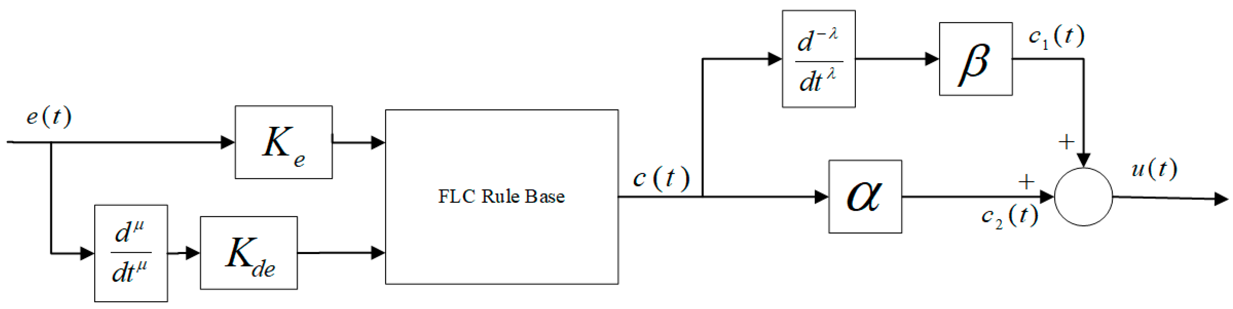
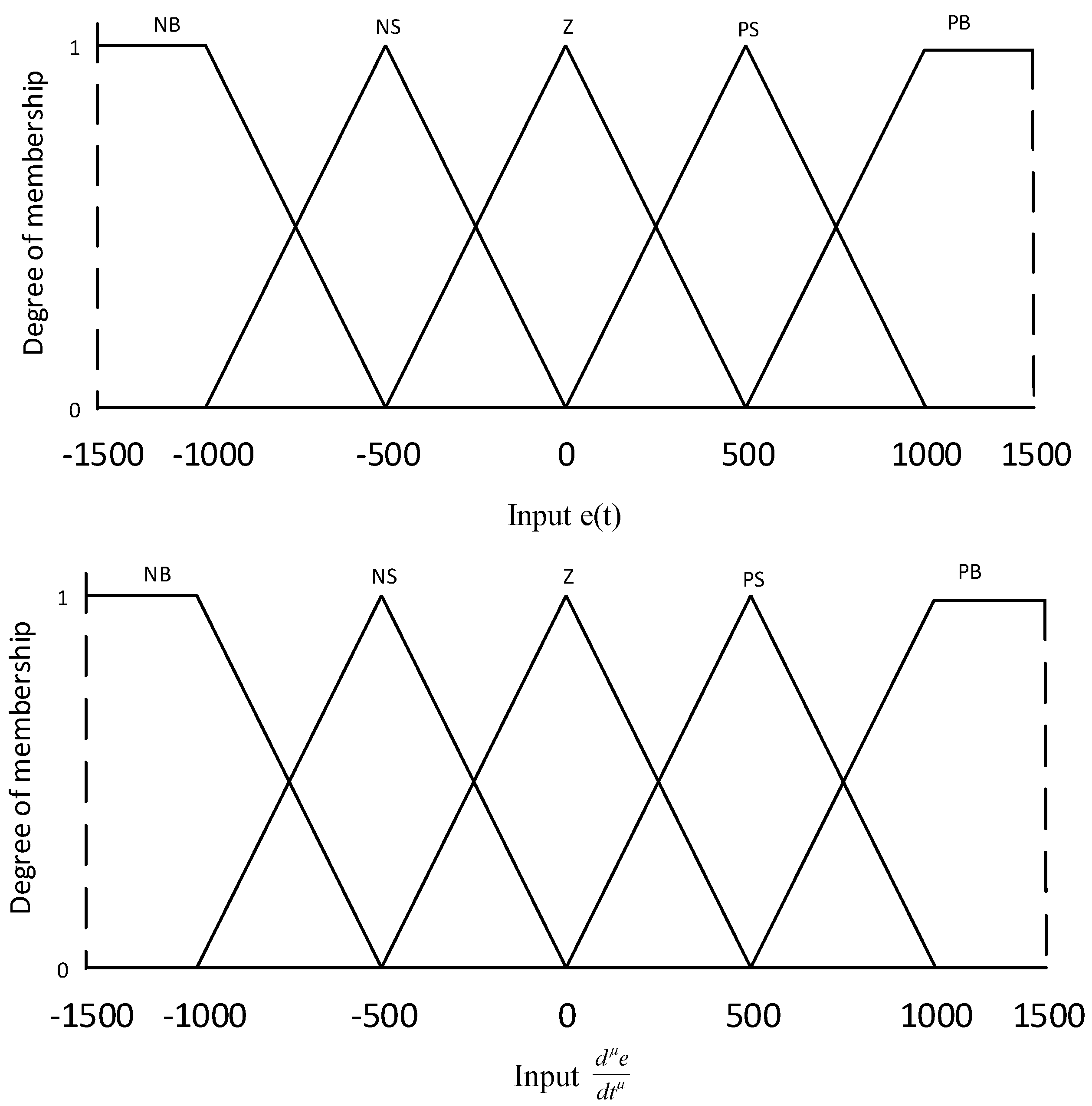
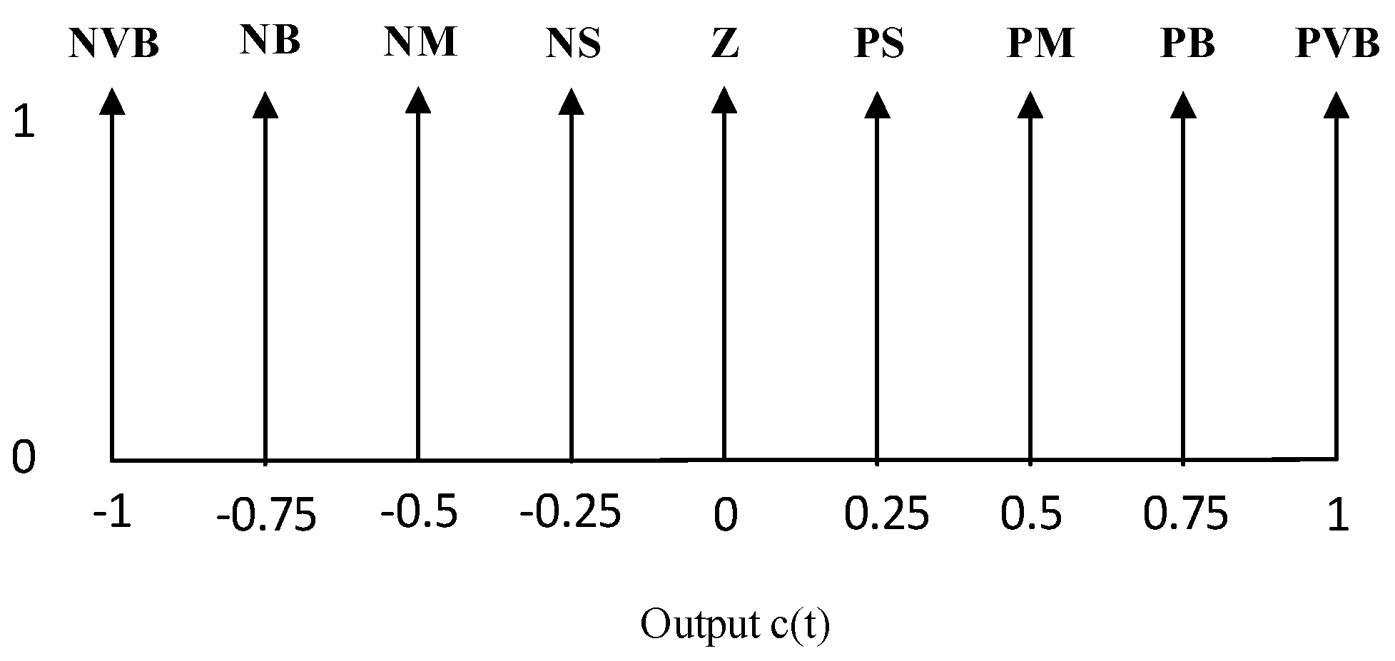
3.1. Fractional Order Fuzzy PID Controller

The control scheme of the FOFPID shown in Figure 4 is a combination of fuzzy PI, and fuzzy PD controllers [19,28], taking K_e and K_de as the input scaling factors, and α and β as output factors. In addition, the differentiation and integration for D and I control can be of fractional orders, such that the control system can be tailored to fulfill the performance requirements.

The parameters $K_e$, $K_{de}$, $\alpha$, and $\beta$ are the PID controller gains, while $\mu$ and $\lambda$ are the orders of differentiation and integration, respectively. The two inputs of the fuzzy logic controller are from the PD control in the front part of this scheme. One is the gain $K_e$ multiplied by the control error $e\left(t\right)$, and the other is $K_{de}$, multiplied by the derivative $\frac{d^{\mu }e}{d{t}^{\mu }}$. The fuzzy controller output $c\left(t\right)$ is subsequently input to the PI control in the rear part. Then the control of the FOFPID can be obtained by

$$u\left(t\right)=\alpha ·c\left(t\right)+\beta ·{{\displaystyle \int }}_0^{t}c\left(\tau \right)d{\tau }^{\lambda }$$

(13)

where $u\left(t\right)$ is the control output. The controller parameters $K_e$, $K_{de}$, $\alpha$, $\beta$, $\mu$, and $\lambda$ need tuning for precise tracking. However, it is hard to tune these gains, especially when using fractional order values. The parameter tuning in this study utilizes an evolutionary computation algorithm, discussed in the next chapter.

In the fuzzy inference system [19], the input and output signals are transformed into fuzzy linguistic variables: PVB (Positive Very Big), NVB (Negative Very Big), PB (Positive Big), NB (Negative Big), PM (Positive Medium), NM (Negative Medium), PS (Positive Small), NS (Negative Small), and Z (Zero), respectively. The membership functions and rule base are shown in Figure 5 and

Table 1. Rule base of the fuzzy logic controller.

c(t)		e(t)
		NB	NS	Z	PS	PB
$\frac{d^{\mu }e}{d{t}^{\mu }}$	NB	NVB	NB	NM	NS	Z
	NS	NB	NM	NS	Z	PS
	Z	NM	NS	Z	PS	PM
	PS	NS	Z	PS	PM	PB
	PB	Z	PS	PM	PB	PVB

. The triangular-shaped membership functions are chosen for the input variables, and singleton functions for the output. The two-dimensional linear rule base shown in Table 1 is used in the fuzzy controller. The inference mechanism is based on the Mamdani algorithm [19] and the rules are expressed by

$$\mathrm{IF} e\left(t\right) \mathrm{is} {\mathrm{A}}^{\mathrm{i}} \mathrm{AND} \frac{d^{\mu }e}{d{t}^{\mu }} \mathrm{is} {\mathrm{B}}^{\mathrm{i}}, \mathrm{THEN} c\left(t\right) \mathrm{is} {\mathrm{C}}^{\mathrm{i}}$$

(14)

where ${\mathrm{A}}^{\mathrm{i}}$, ${\mathrm{B}}^{\mathrm{i}}$, and ${\mathrm{C}}^{\mathrm{i}}$ are the linguistic labels of these linguistic variables $e\left(t\right)$,$\frac{d^{\mu }e}{d{t}^{\mu }}$ and $c\left(t\right)$, and are characterized by membership functions for each variable. Here the max–min composition is used, and a fuzzy set $u\left(F\right)$ can be inferred from the following relation:

$$u\left(F_i\right)=\underset{i=1}{\overset{K}{{\displaystyle \cup }}}\left(u^{\mathrm{i}}\left(\mathrm{A}\right){\displaystyle \cap }{u}^{\mathrm{i}}\left(\mathrm{B}\right)\right)$$

(15)

where K denotes the number of fuzzy output sets, and $u^{\mathrm{i}}\left(\mathrm{A}\right)$ and $u^{\mathrm{i}}\left(\mathrm{B}\right)$ are the MFs of the fuzzy sets A and B, respectively. ${\displaystyle \cap }$ and ${\displaystyle \cup }$ denote the min function (T-norm) and max function (T-conorm), respectively. $F_i$ represents the value of the i-th output MF, and $u\left(F_i\right)$ is its membership value at the i-th quantization level. The center-average defuzzification is utilized here to obtain the output $c\left(t\right)$, as follows:

$$c\left(t\right)=\frac{{{\displaystyle \sum }}_{i=1}^K{F}_{i}u\left(F_i\right)}{{{\displaystyle \sum }}_{i=1}^{K}u\left(F_i\right)}$$

(16)

Oustaloup’s recursive filter [29] is utilized here to implement the fractional-order elements $s^{\lambda }$ ($\lambda \in \left[-1,1\right]\subseteq \Re$). The filter is given by

$$G_f\left(s\right)=s^{\lambda }=K{\displaystyle \prod }_{k=-N}^N\frac{s+{\omega }_k^{\prime }}{s+{\omega }_k}$$

(17)

where the poles and zeros can be recursively evaluated by

$${\omega }_k\prime ={\omega }_b{\left(\frac{{\omega }_h}{{\omega }_b}\right)}^{\frac{k+N+\frac{1}{2}\left(1-\lambda \right)}{2N+1}}, {\omega }_k={\omega }_b{\left(\frac{{\omega }_h}{{\omega }_b}\right)}^{\frac{k+N+\frac{1}{2}\left(1+\lambda \right)}{2N+1}}, K={\omega }_h^{\lambda }$$

(18)

The output of this filter is an approximation of a fractionally diff-integrated signal. $\lambda$ is the order of the differ-integration, [${\omega }_b, {\omega }_h$] is the preset frequency range (rad/s), and N is the order of the approximate integer-order transfer function. The selected parameters for Oustaloup’s recursive filter used in this work are ${\omega }_b=0.001, {\omega }_h=100, N=3$.

3.2. The Objective Function

Figure 6 shows the FOFPID control scheme. It consists of two subsystems: one is the X-axis control loop, and the other is the Y-axis control loop, which possesses a mechanical coupling effect. The design of this control scheme is to reduce X- and Y-axis tracking errors, and also reduce the synchronous error in the Y-axis. To achieve this purpose with an optimization algorithm, a fitness function containing these error terms should be minimized. The ITAE performance criterion [30] is used to be the fitness function and is expressed as

$$\mathrm{ITAE}={{\displaystyle \int }}_0^{T}t\left|e\left(t\right)\right|dt$$

(19)

where $e\left(t\right)$ denotes the tracking error at instant t.

In the control design, compared to the IAE (integral of the absolute error) and ISE (integral square error) indices, the ITAE performance index has smaller oscillations and overshoots. There are eighteen tuning parameters in the control scheme: (1) $K_e$, $K_{de}$, $\alpha$, $\beta$, $\mu$, and $\lambda$ for the X-axis, (2) $K_{e1}$, $K_{de1}$, ${\alpha }_1$, ${\beta }_1$, ${\mu }_1$, and ${\lambda }_1$ for the master Y-axis, and (3) $K_{e2}$, $K_{de2}$, ${\alpha }_2$, ${\beta }_2$, ${\mu }_2$, and ${\lambda }_2$ for the slave Y-axis. To find appropriate parameters for the controller scheme, optimization algorithms can be used. For the gantry system described in Figure 4, the optimization problem is to minimize the system $\mathrm{ITAE}$ index. The ITAE of the whole system should consider the tracking errors for X-axis $e_X\left(t\right)$, master Y-axis $e_{YM}\left(t\right)$, and slave Y-axis $e_{YS}\left(t\right)$, and the synchronous error, which is the difference of two Y-axes $e_{YM}\left(t\right)$. Thus, the ITAE is given as

$$\mathrm{ITAE}=\frac{1}{4}({\displaystyle \sum }_{\mathrm{r}=1}^4{\mathrm{ITAE}}_r)$$

(20)

with ${\mathrm{ITAE}}_1={{\displaystyle \int }}_0^{T}t\left|e_X\left(t\right)\right|dt$, ${\mathrm{ITAE}}_2={{\displaystyle \int }}_0^{T}t\left|e_{YM}\left(t\right)\right|dt$, ${\mathrm{ITAE}}_3={{\displaystyle \int }}_0^{T}t\left|e_{YS}\left(t\right)\right|dt$, ${\mathrm{ITAE}}_4={{\displaystyle \int }}_0^{T}t\left|e_{YMS}\left(t\right)\right|dt$.

4. Optimization Algorithms

To choose the controller parameters, four evolutionary computations are tested and compared: particle swarm optimization (PSO), invasive weed optimization (IWO), a gray wolf optimizer (GWO), and biogeography-based optimization (BBO). The objective functions for the optimal algorithms can be formulated with the aim of minimizing the ITAE index. The time multiplication term in the ITAE index helps to reduce the settling time, for the penalty increases with time.

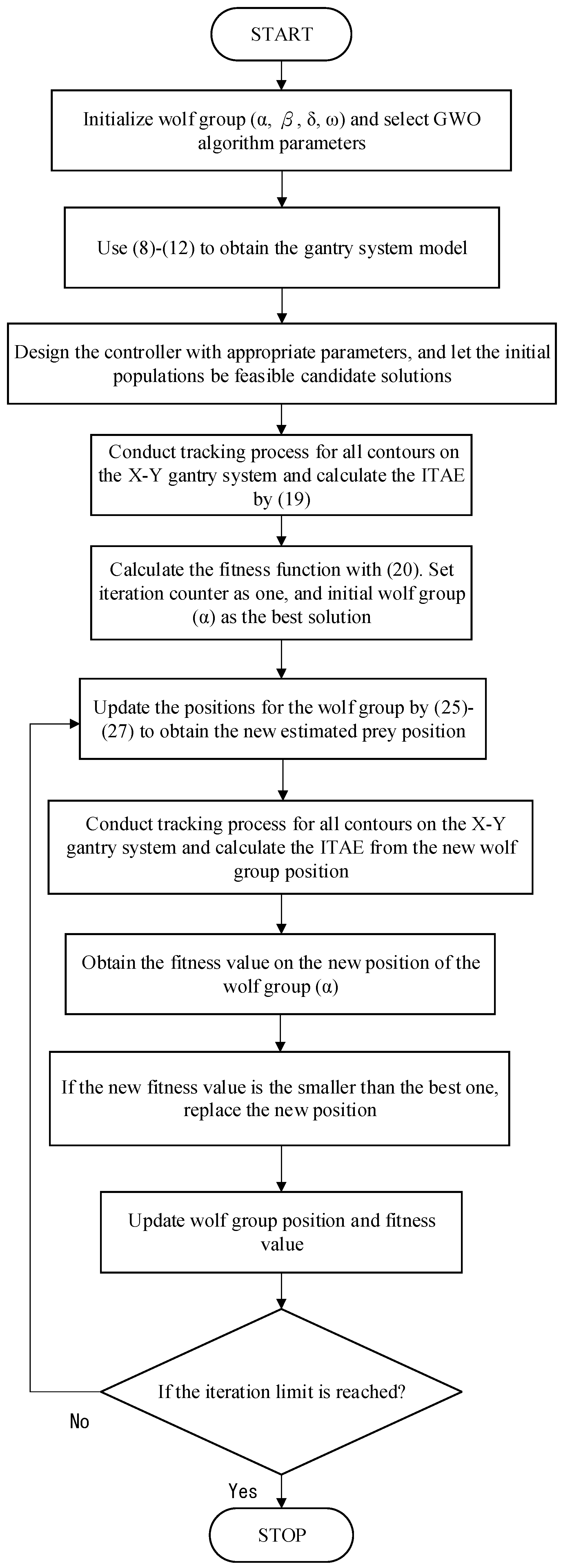
4.1. Grey Wolf Optimizer (GWO) Algorithm

A grey wolf optimizer [22] is an intelligent group optimization algorithm proposed by Mirjalili et al. of Griffith University, Australia, in 2014. The algorithm is an optimized search method inspired by the behavior of gray wolves when they hunt prey. The levels of the gray wolf social hierarchy are separated into $\alpha , \beta , \delta , \mathrm{and} \omega$ from top to bottom. Wolf α represents the fittest solution, whereas the second and third best solutions are β and δ, respectively. The remaining wolves, ω, are candidate solutions. The GWO procedure has three steps: encircling, hunting, and attacking. The encircling behavior is modeled by the following equations:

$$\overrightarrow{D}=\left|\overrightarrow{C}·\overrightarrow{X_p}\left(t\right)-\overrightarrow{X}\left(t\right)\right|$$

(21)

$$\overrightarrow{X}\left(t+1\right)=\overrightarrow{X_p}\left(t\right)-\overrightarrow{A}·\overrightarrow{D}$$

(22)

where t denotes the current iterations, $\overrightarrow{X}$ is the position vector of a grey wolf, $\overrightarrow{X_p}$ is the position vector of the prey, and $\overrightarrow{A}$ and $\overrightarrow{C}$ are coefficient vectors calculated by

$$\overrightarrow{A}=2\overrightarrow{a}·\overrightarrow{r_1}-\overrightarrow{a}$$

(23)

$$\overrightarrow{C}=2·\overrightarrow{r_2}$$

(24)

where $\overrightarrow{a}$ is the convergence factor, decreasing linearly from 2 to 0 in the iterative process, and $\overrightarrow{r_1}$ and $\overrightarrow{r_2}$ are random vectors on the range [0, 1]. The outcome of these equations is that the random vectors $\overrightarrow{r_1}$ and $\overrightarrow{r_2}$ allow wolves to reach any position around the prey.

In the hunting stage, the first three best solutions obtained so far are saved, and other wolves are forced to update their positions according to the best agent. The position update equations are as follows:

$$\overrightarrow{D_{\alpha }}=\left|\overrightarrow{C_1}·\overrightarrow{X_{\alpha }}-\overrightarrow{X}\right|, \overrightarrow{D_{\beta }}=\left|\overrightarrow{C_2}·\overrightarrow{X_{\beta }}-\overrightarrow{X}\right|, \overrightarrow{D_{\delta }}=\left|\overrightarrow{C_3}·\overrightarrow{X_{\delta }}-\overrightarrow{X}\right|$$

(25)

$$\overrightarrow{X_1}=\overrightarrow{X_{\alpha }}-\overrightarrow{A_1}·\left(\overrightarrow{D_{\alpha }}\right), \overrightarrow{X_2}=\overrightarrow{X_{\beta }}-\overrightarrow{A_2}·\left(\overrightarrow{D_{\beta }}\right), \overrightarrow{X_3}=\overrightarrow{X_{\delta }}-\overrightarrow{A_3}·\left(\overrightarrow{D_{\delta }}\right)$$

(26)

$$\overrightarrow{X}\left(t+1\right)=\frac{\overrightarrow{X_1}+\overrightarrow{X_2}+\overrightarrow{X_3}}{3}$$

(27)

The final stage of hunting is to “attack the prey” (obtain the optimal solution). As iterations progress, the value of $\overrightarrow{a}$ decreases from 2 to 0, pushing the wolves to approach the prey. Note that the range of $\overrightarrow{A}$ is related to the value of $\overrightarrow{a}$. When $\left|\mathrm{A}\right|<1$, the wolves are forced to attack toward the prey.

With the GWO algorithm, the optimal control parameters of the proposed FOFPID controller can be found. The procedure is described as follows:

(1)

Initialize the wolf group ($\alpha , \beta ,\delta ,\omega$) and select the GWO algorithm parameters.

(2)

Design the appropriate parameters ($K_e$, $K_{de}$, $\alpha$, $\beta$, $\mu$, $\lambda$, $K_{e1}$, $K_{de1}$, ${\alpha }_1$, ${\beta }_1$, ${\mu }_1$, ${\lambda }_1$, $K_{e2}$, $K_{de2}$, ${\alpha }_2$, ${\beta }_2$, ${\mu }_2$, ${\lambda }_2$), and let the initial populations be feasible candidate solutions.

(3)

Conduct the tracking process for all contours on the X–Y gantry system, calculate the ITAE, and then calculate the fitness function with (20).

(4)

Set the iteration counter as one and the initial wolf group ($\alpha$) as the best solution.

(5)

Update the positions for the wolf group by (25)–(27) to obtain the new estimated prey position.

(6)

Again, perform all contour tracking for the X–Y gantry system, compute the ITAE, and calculate the fitness value according to the new wolf group ($\alpha$) position.

(7)

Check whether the new fitness value is smaller than the best one. If the new fitness value is smaller, then replace the new position with it.

(8)

Update the wolf group position and the corresponding fitness values.

(9)

If the iteration limit is not reached, increase the iteration counter and return to Step (5).

These steps can also be represented as a flow chart as shown in Figure 7.

4.2. Other Optimization Algorithms

To investigate the effects of different optimization algorithms on the proposed FOFPID controller, three other optimization algorithms are tested for comparison: IWO, PSO, and BBO. In the experimental results, the comparisons of the four algorithms are demonstrated.

IWO is an effective global optimization algorithm proposed by A. Mehrabian and C. Lucas [21] in 2006. It is a numerical stochastic optimization algorithm evolved from the principle of the rapid reproduction and growth of weeds in nature. The IWO process first initializes the growth and reproduction of weeds, then updates the best fitness of weeds with a distribution equation, and finally runs a number of iterations.

The PSO algorithm is a modem heuristic algorithm developed by Kennedy and Eberhart in 1995 [20]. It formulates the optimization problems as bird flocking behavior. In the PSO algorithm, each particle in the search space stands for a solution to the optimization problem. Each particle possesses a fitness value and velocity to determine the distance and direction of its movement. Then the particles follow the particle with the best fitness values to search in the solution space. To implement this method, initialize a population of particles, then update the particle locations, and iterate to produce an optimal solution.

The BBO approach was published by Dan Simon [23] in 2008. It uses the distribution of species between neighboring islands to construct a mathematical model for species extinction and migration. The process of optimization is as follows: initialize a habitat, update that optimal habitat’s suitability using given migration and mutation rates, and then iterate and update the process to obtain a solution.

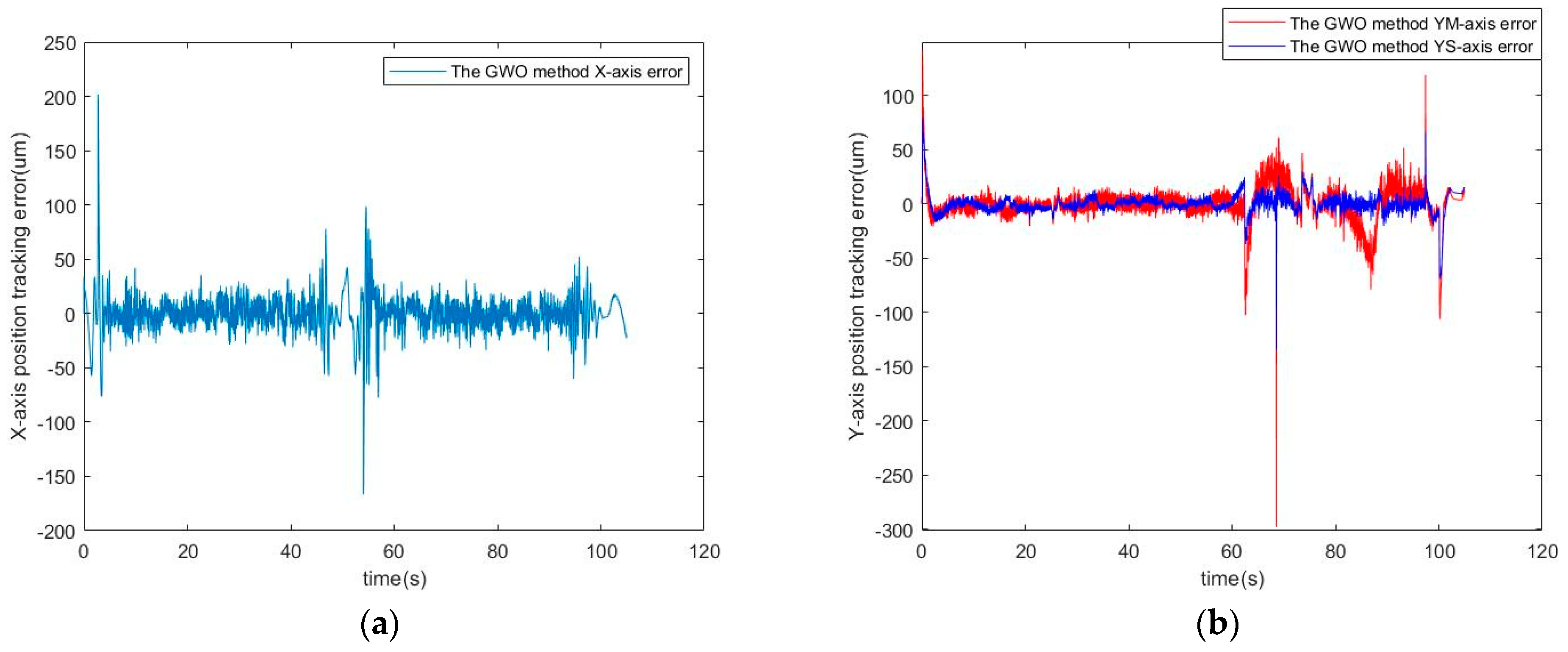
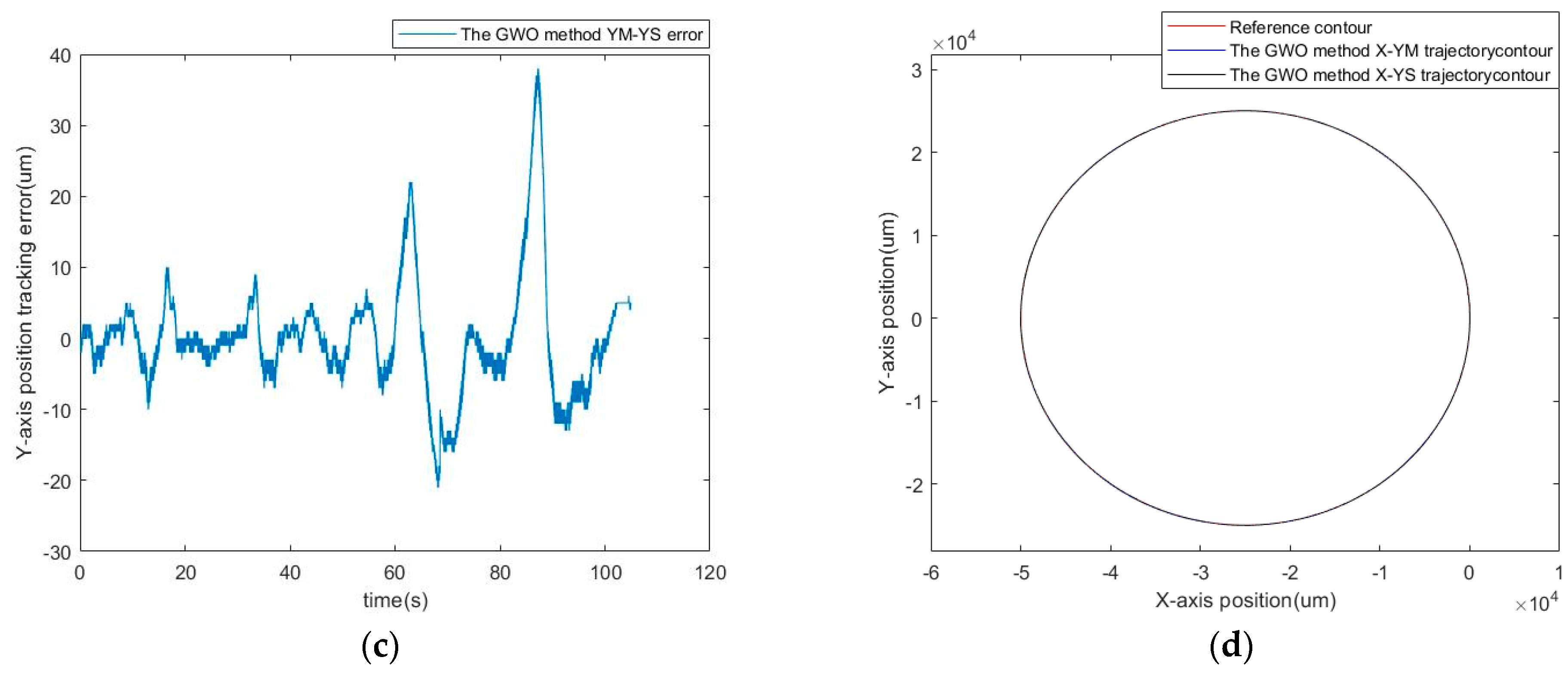
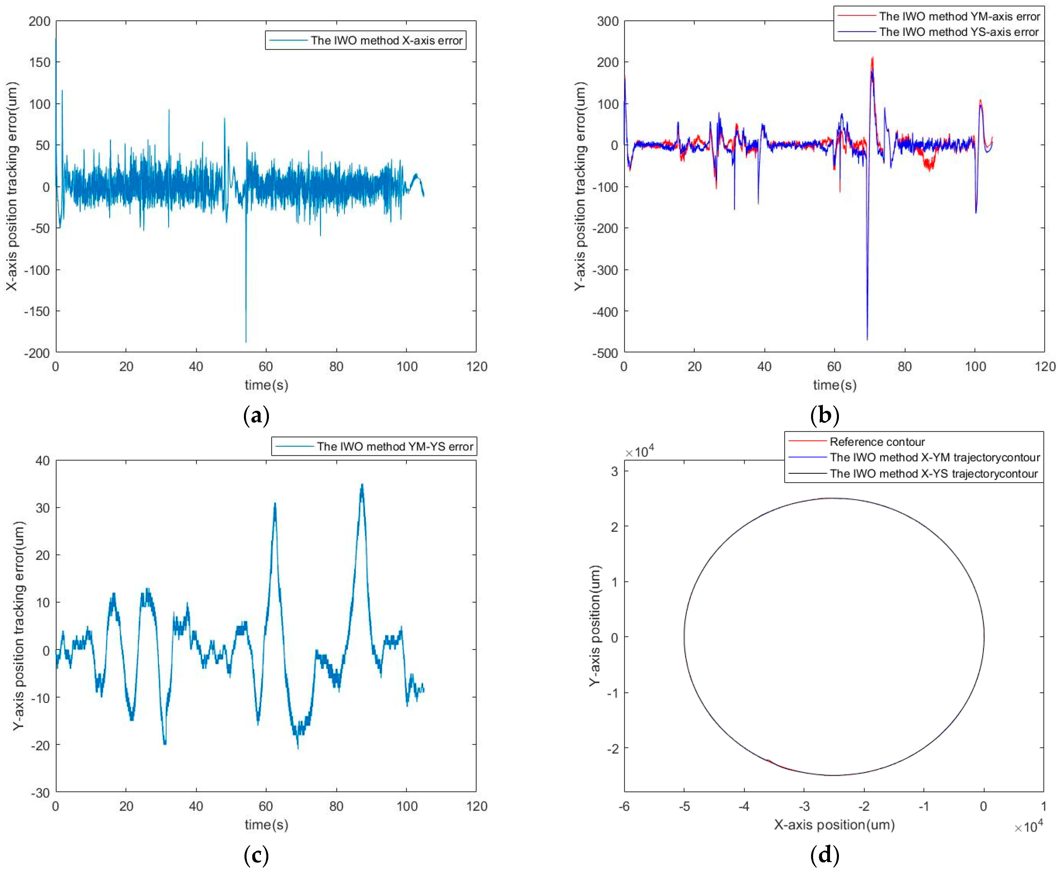
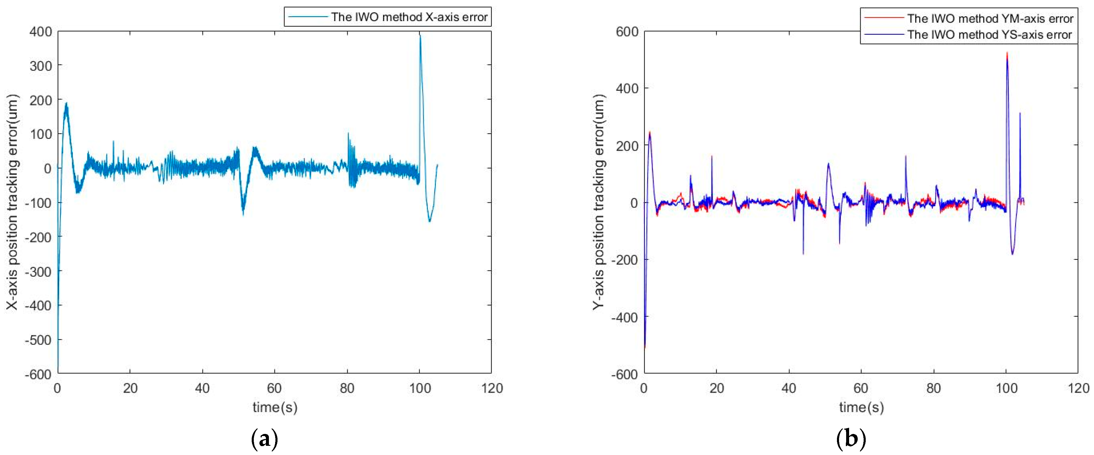
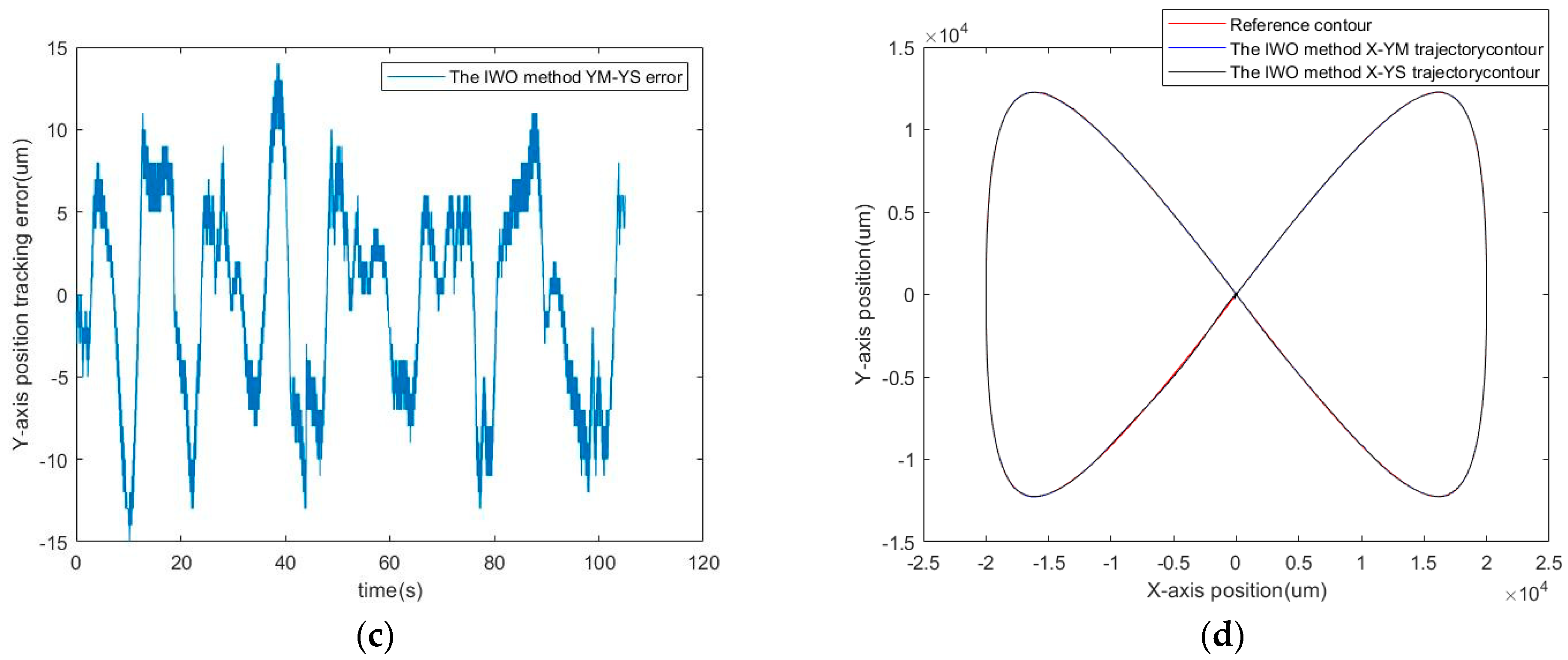
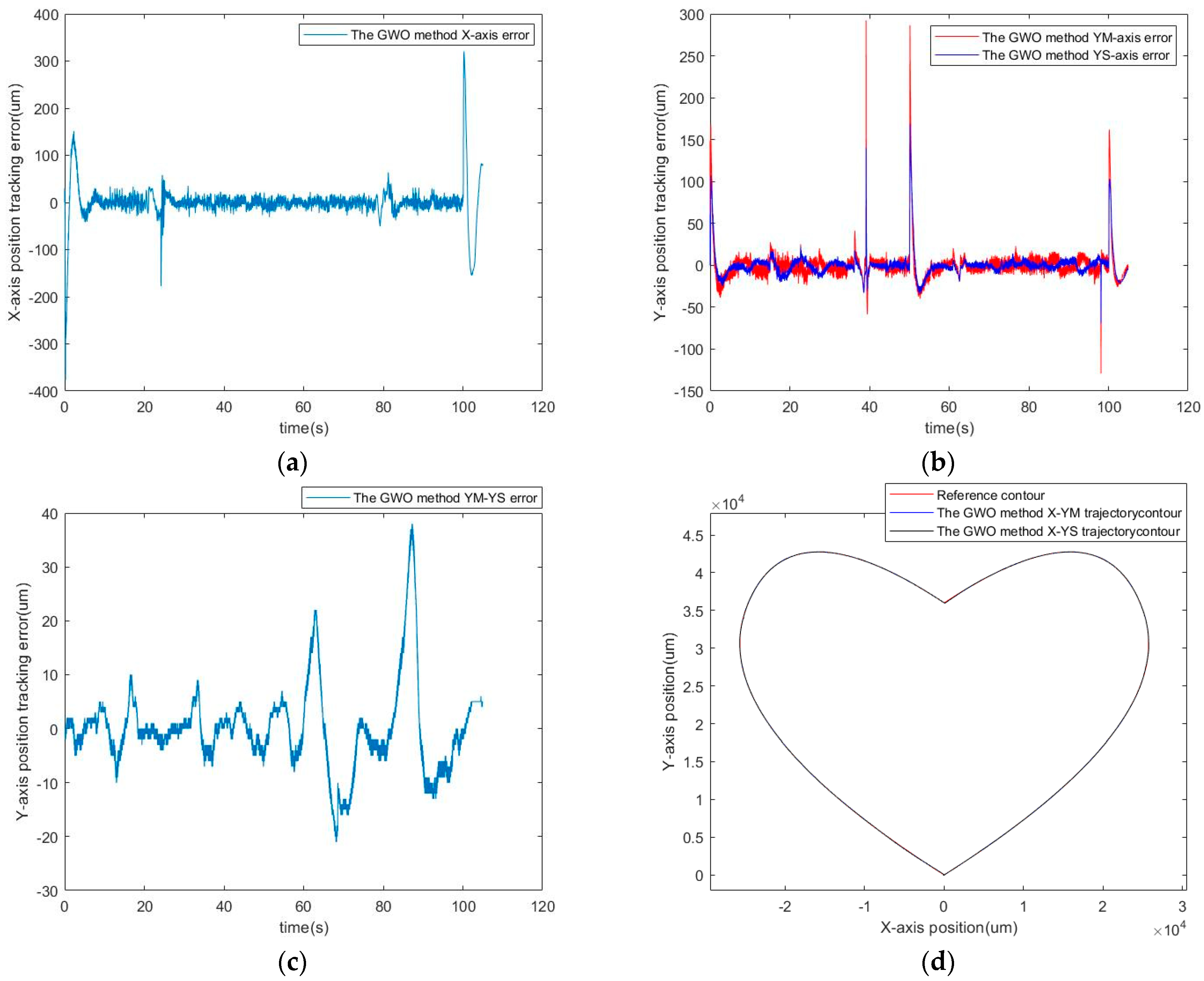
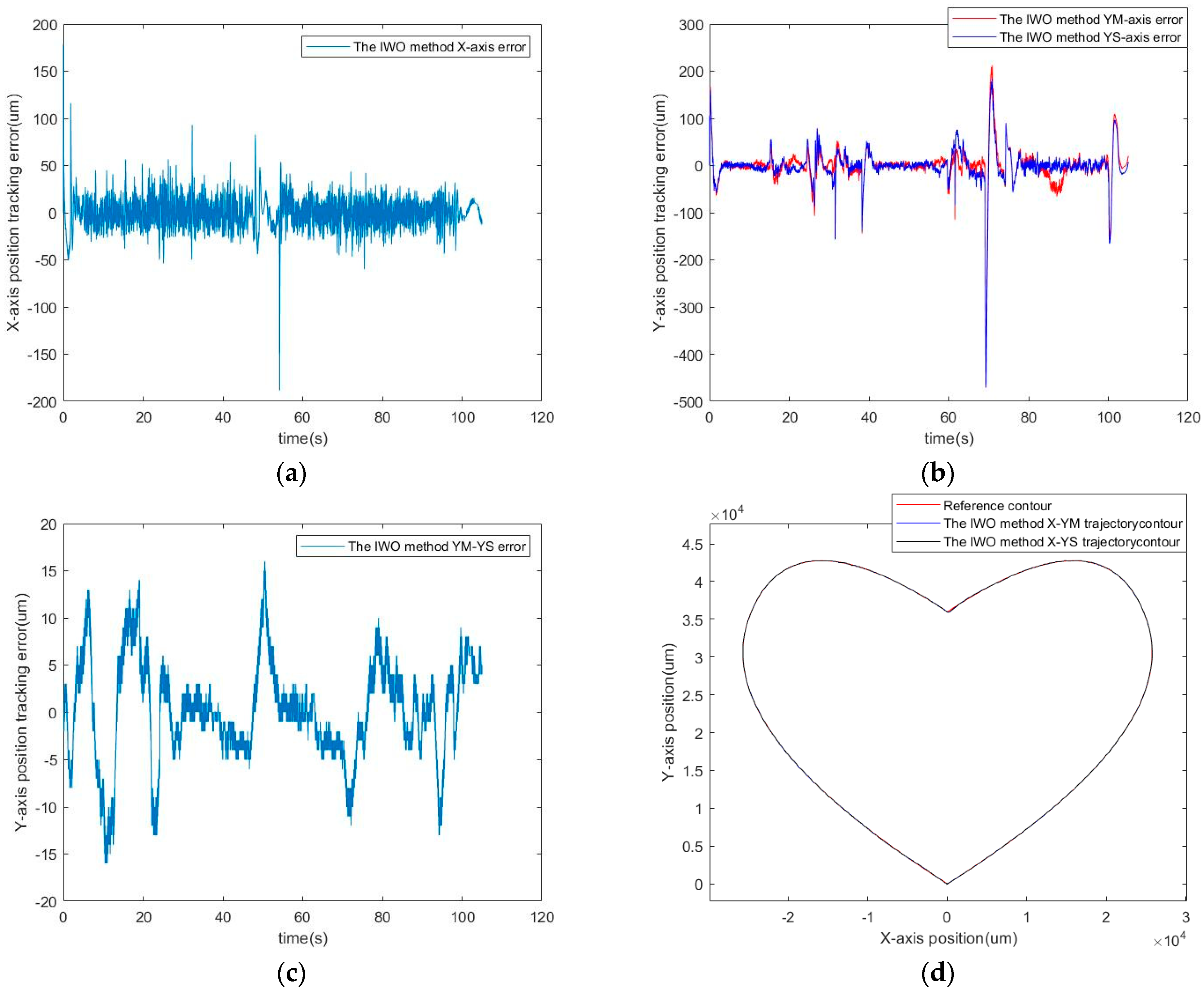
5. Experimental Results

The setup of the gantry-type platform is shown in Figure 2. The PMLSMs are CPC-CLS-PM4 from Chieftek Precision Co., Ltd. and are actuated by the COR-5/230, which is a PWM digital servo driver manufactured by Elmo Motion Control. The peak and continuous force of the PMLSM are 74 N and 18.5 N. Its magnetic pole pitch and continuous current are 15 mm and 5 A, respectively. The platform consists of two parallel motors on the Y-axis and another one on the X-axis. A mechanical coupling happens on the Y-axis for these two motors. Optical encoder sensors provide the measurement of the displacement on each axis. The signals are transferred with an encoder card for position feedback while a D/A converter card charges for control. The optical encoders are set up to measure the displacements with the resolution of 1 μm. The sampling rate of the practical controller is 1 KHz. Both the X- and Y-axes possess a stroke of 225 mm.

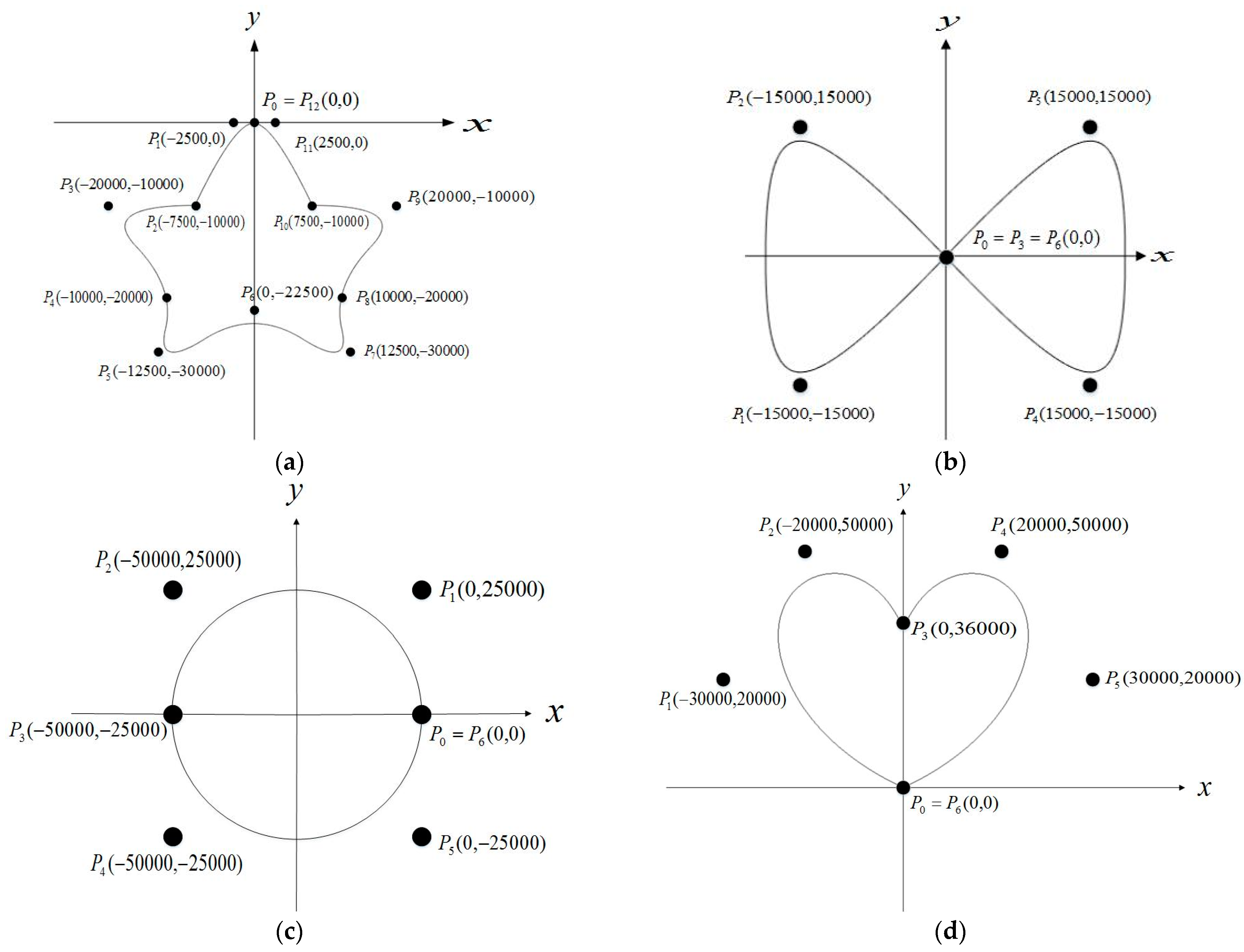
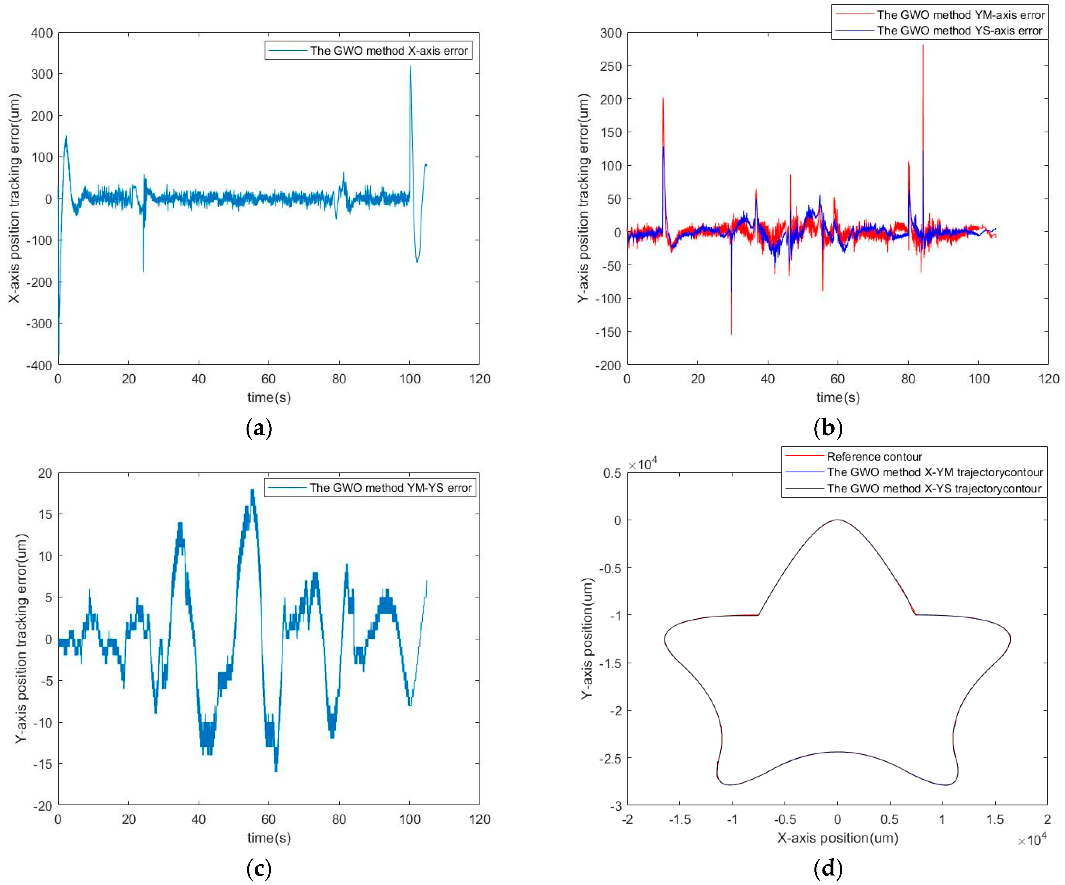
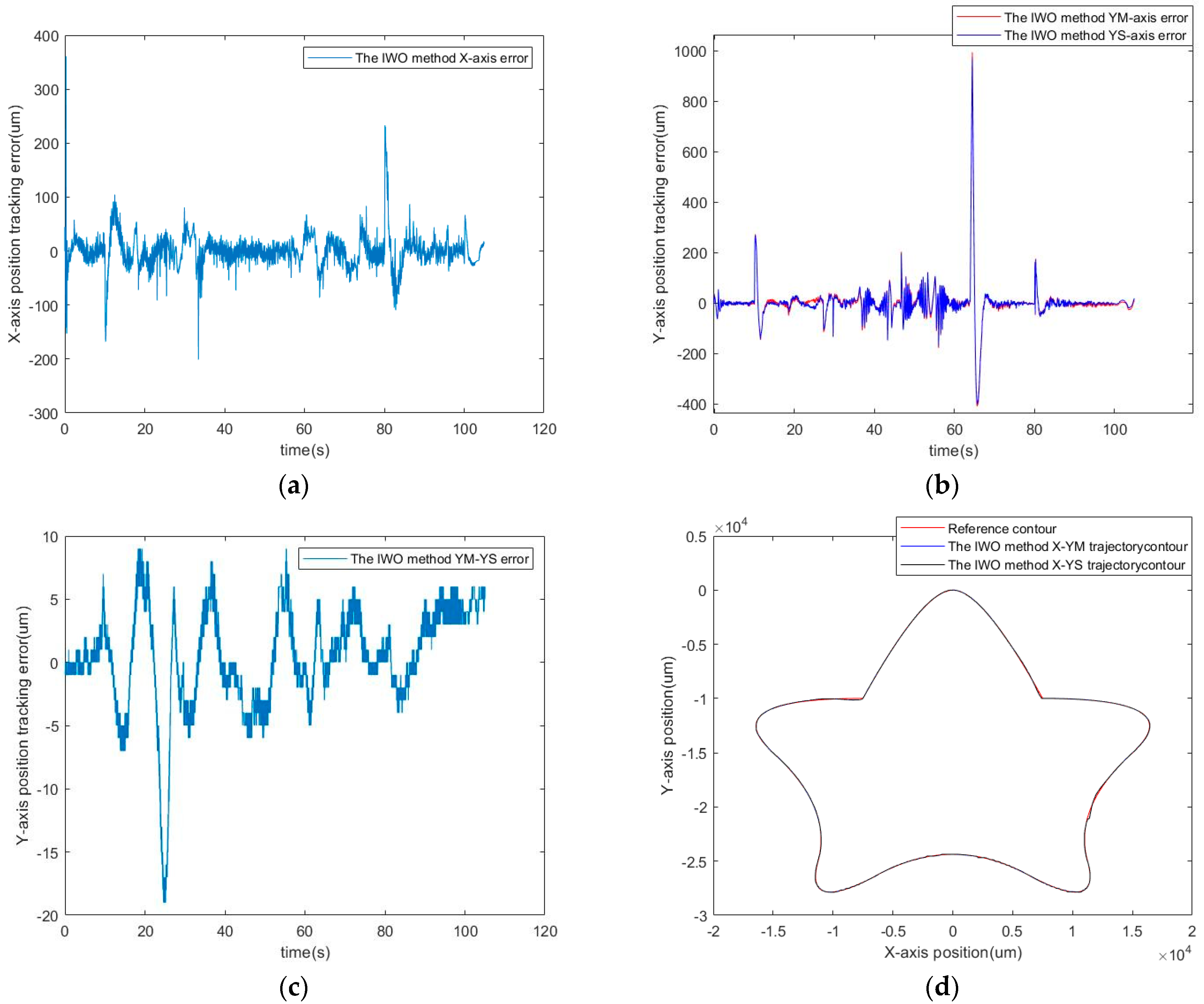
5.1. Contour Planning

The contours in the simulations and experiments are planned by the non-uniform rational B-spline (NURBS), which is a parametric curve composed of parameters such as control point, knot vector, degree of curve, and weight [31,32,33]. The NURBS curves can be modified by adjusting the weights and control points, or by changing the basis function generated by the recursive calculation through different spacing of the elements in the node vector. This means a NURBS-generated curve can be divided into a string of multi-interval fitted splines. The equation for defining a NURBS curve is

$$C\left(u\right)=\frac{{{\displaystyle \sum }}_{i=0}^n{B}_{i,d}\left(u\right)W_i{P}_i}{{{\displaystyle \sum }}_{i=0}^n{B}_{i,d}\left(u\right)W_i}={\displaystyle \sum }_{i=0}^n{R}_{i,d}\left(u\right)P_i$$

(28)

where $P_i$ denotes the control point, $R_{i,d}\left(u\right)$ is the rational basis function, $B_{i,d}\left(u\right)$ is the basis function, $W_i$ is the weight, and d and u are the degree and parameter of the NURBS curve, respectively.

Table 2. NURBS parameters for the four contours.

Trajectory Type	NURBS Parameters
Circle	d = 2, P = [(0,0),(0, 25,000), (−50,000, 25,000),(−50,000, 0), (−50,000, −25,000), (0, −25,000), (0, 0)], k = [0, 0, 0, 0.25, 0.5, 0.5, 0.75, 1, 1, 1], w = [1, 0.5, 0.5, 1, 0.5, 0.5, 1]
Heart	d = 2, P = [(0,0), (−30,000, 20,000), (−20,000, 50,000), (0, 36,000), (20,000, 50,000), (30,000, 10,000), (0,0)], k = [0, 0, 0, 0.25, 0.5, 0.5, 0.75, 1, 1, 1], w = [1, 1, 1, 1, 1, 1, 1]
Bow	d = 2, P = [(0, 0), (−15,000, −15,000), (−15,000, 1.5), (0, 0), (15,000, −15,000), (15,000, 150,000), (0, 0)], k = [0, 0, 0, 0.25, 0.5, 0.5, 0.75, 1, 1, 1], w = [1, 2.5, 2.5, 1, 2.5, 2.5, 1]
Star	d = 2, P = [(0, 30,000), (−2500, −30,000), (−7500, 20,000), (−20,000, 20,000), (−1000, 10,000), (−12,500, 0), (0, 7500),(12,500, 0),(10,000, 10,000), (20,000, 20,000), (7500, 20,000),(2500, 30,000),(0, 30,000)], k = [0, 0, 0, 0.1, 0.1, 0.2, 0.3, 0.4, 0.5, 0.6, 0.7, 0.8, 0.8, 1, 1, 1], w = [1, 1, 1, 1, 1, 1, 1, 1, 1, 1, 1, 1, 1]

shows the NURBS parameters of each contour. As shown in Figure 8a, the star NURBS can be designed with 12 control points. Figure 8b–d shows the NURBS control points for a circle, a bow, and a heart, respectively.

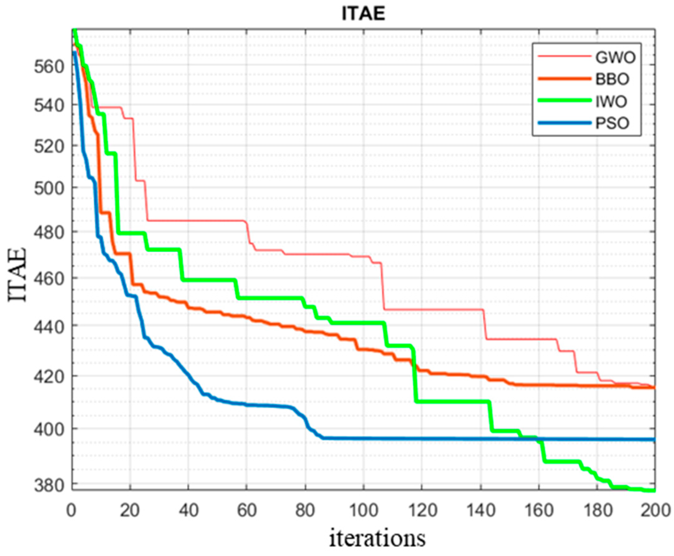
5.2. Optimization and Performance Indices

MATLAB and Simulink are used to complete the simulations. Simulations are conducted based on the identified dynamic model (8)–(12), which represents the gantry platform. All four optimization methods are tested: (1) PSO, (2) IWO, (3) GWO, and (4) BBO. These optimization algorithms are employed to tune the parameters in the FOFPID controller based on the ITAE criterion. To evaluate the ITAE for the four contour types, the average is calculated by

$$\mathrm{ITAE}=\frac{{\mathrm{ITAE}}_{\mathrm{C}}+{\mathrm{ITAE}}_{\mathrm{B}}+{\mathrm{ITAE}}_{\mathrm{S}}+{\mathrm{ITAE}}_{\mathrm{H}}}{4}$$

(29)

where the subscripts of ${\mathrm{ITAE}}_{\mathrm{X}}$ denote the contour types circle, bow, star, and heart, respectively. The number of iterations for each scheme is limited to 200.

Table 3. Parameters of the optimization algorithms.

Optimization Algorithm	Parameters
PSO	population size: $N=30$ leaning parameters: $c_1=1.2$, $c_2=1.2$ upper/lower bounds of the random velocity weight: $v_{max}^j=0.72$, $v_{min}^j=-0.72$ upper/lower bound of the position: $x_{max}^j=1.9$, $x_{max}^j=0.1$
IWO	population size: $N=30$ maximum group size $ite{r}_{max}$ = 30 nonlinear harmonic parameter $n=2$ initial standard deviation ${\sigma }_i$ = 0.5 final standard deviation ${\sigma }_i$ = 0.001 upper/lower bound of weed seeds: $1.9$/$0.1$
GWO	population size: $N=30$ upper/lower bound of wolf group(alpha): $1.9/0.1$
BBO	number of habitats: $N=30$ max/min migration rates: $E=I=1$, $m_{max}$ = 0.1 upper/lower bound of habitat species: $1.9/0.1$

shows the parameters used in the optimization process.

Two indexes, the tracking error standard deviation (TESD) and average tracking error (ATE) are employed to evaluate the performances of both the simulations and experiments. These indexes are defined by

(1)

ATE:

$$m={\displaystyle \sum }_{k=1}^n\frac{e\left(k\right)}{n}$$

(30)

with $e\left(k\right)=\sqrt{e_x^2\left(k\right)+e_y^2\left(k\right)}$ where $e_x\left(k\right)$ and $e_y\left(k\right)$ are the tracking errors in the X- and Y-axis. As there are two slides on the Y-axis, the tracking error becomes $e_y\left(k\right)=\frac{e_{ym}\left(k\right)+e_{ys}\left(k\right)}{2}$, and n denotes the number of all contour points.

(2)

TESD:

$$T_s=\sqrt{\frac{{{\displaystyle \sum }}_{k=1}^n{\left(T\left(k\right)-m\right)}^2}{n}}$$

(31)

The ATE and TESD indices are often used to measure contour tracking performance. The former is used to measure the capability of trajectory tracking, while the latter can evaluate the oscillation.

5.3. Simulation Results

Figure 9 shows the curves of ITAE in the iterations of optimization for the four methods. Among them, PSO has the fastest decline, but IWO eventually approaches a lower value.

Table 4. Optimal scaling factor parameters for all trajectory types.

value	$K_e$	$\mu$	$K_{de}$	$\lambda$	$\beta$	$\alpha$
PSO	1.8931	0.1097	0.4520	1.5940	1.9000	0.9726
IWO	1.8237	0.2757	1.8330	1.6256	1.4351	1.1889
BBO	1.8980	0.1006	1.8914	1.6927	1.9000	0.6967
GWO	1.3132	0.1285	1.8970	1.6103	1.8326	1.0344
value	$K_{e1}$	${\mu }_1$	$K_{de1}$	${\lambda }_1$	${\beta }_1$	${\alpha }_1$
PSO	0.4488	0.1000	1.9000	1.4877	1.9000	0.8245
IWO	1.8866	0.1012	1.6841	1.5311	1.8837	0.7184
BBO	1.7297	0.4819	0.7888	1.4647	1.6594	0.8007
GWO	1.8825	0.1085	1.4989	1.3023	1.8645	1.4217
value	$K_{e2}$	${\mu }_2$	$K_{de2}$	${\lambda }_2$	${\beta }_2$	${\alpha }_2$
PSO	1.2828	0.142	1.9000	1.4889	1.4156	0.6118
IWO	1.8302	0.1000	1.7325	1.5320	1.9000	0.7267
BBO	1.8914	0.4146	1.1917	1.4872	1.3578	0.6606
GWO	1.8992	0.2610	1.7539	1.3435	1.8493	1.3241

shows the optimal learning parameters corresponding to the PSO, IWO, BBO, and GWO methods. Common optimal parameters are employed in each simulation result, and the tracking errors are compared and summarized.

Table 5. The simulation results of all trajectories.

Method	$\mathbf{ATE} (\mathbf{\mu }\mathbf{m}$)	$\mathbf{TESD} (\mathbf{\mu }\mathbf{m}$)	ITAE
Circle
PSO	1.4719	3.2174	728.4400
IWO	0.9100	1.6635	689.4438
BBO	1.5367	3.0456	732.9247
GWO	1.1919	1.4536	732.1176
Heart
PSO	1.3767	7.3135	687.1533
IWO	1.2314	5.5600	662.0899
BBO	1.4962	7.7701	706.2485
GWO	1.2854	4.7161	716.1556
Star
PSO	2.9381	9.7067	758.2886
IWO	2.9195	6.0844	732.7888
BBO	2.9834	9.8334	822.2761
GWO	2.8224	6.8502	800.8768
Bow
PSO	6.2185	30.6246	726.3240
IWO	2.0803	12.5113	686.4565
BBO	5.9139	27.0573	778.0170
GWO	5.0548	18.6534	795.2960
Average
PSO	3.0013	12.7156	725.0515
IWO	1.7852	6.4548	692.6948
BBO	2.9826	11.9266	759.8666
GWO	2.5886	7.9183	761.1115

shows the comparison of the simulation results for the optimization algorithms. Taking an average of all four contours, the IWO method achieved a higher accuracy, with an ATE of 1.7852 $\mathsf{\mu }\mathrm{m}$, TESD of 6.4548 $\mathsf{\mu }\mathrm{m}$, and ITAE of 692.6948.

5.4. Experimental Results

The real-time control experiments are conducted to verify the performance of the proposed method. Figure 10 and Figure 11, respectively, show the star position error trajectories using the GWO and IWO algorithms. The controller parameters are obtained from the optimization process in the simulations. Figure 10a and Figure 11a illustrate the tracking errors on the X-axis, Figure 10b and Figure 11b show the tracking errors of the master and slave Y-axes together, and Figure 10c and Figure 11c show the synchronization errors, which are within 20 $\mathsf{\mu }\mathrm{m}$ and decay gradually. Figure 10d and Figure 11d demonstrate the contour trajectories. The smooth trajectories and small steady-state error can be seen in the results. The circle contour tracking results using the GWO and IWO algorithms are shown in Figure 12 and Figure 13, respectively. Figure 12c and Figure 13c show the synchronization errors, which are always within 40 $\mathsf{\mu }\mathrm{m}$. Figure 14 and Figure 15 are the position error trajectories of the bow tie with GWO and IWO, respectively. Figure 14c and Figure 15c show that the synchronization errors are within 12 $\mathsf{\mu }\mathrm{m}$ and 15 $\mathsf{\mu }\mathrm{m}$, respectively. The heart contour tracking results are shown in Figure 16 and Figure 17. The synchronization errors are shown in Figure 16c and Figure 17c, and are within 40 $\mathsf{\mu }\mathrm{m}$ and 15 $\mathsf{\mu }\mathrm{m}$, respectively.

The ATE and TESD tracking indices for the star, circle, bow, and heart contours are displayed in

Table 6. The experimental results of all trajectories.

Method	ATE ($\mathbf{\mu }\mathbf{m}$)	TESD ( $\mathbf{\mu }\mathbf{m}$)	ITAE
Circle
PSO	12.33468	19.06461	1000.13697
IWO	22.55877	39.85242	1018.96457
BBO	13.65512	15.22419	1009.078
GWO	7.93084	8.69547	998.86251
Heart
PSO	17.05340	23.22570	1011.88779
IWO	23.88164	36.07943	1015.39364
BBO	18.09240	27.08182	1008.25875
GWO	9.09414	16.49567	994.75943
Star
PSO	19.17965	21.18270	997.62259
IWO	23.93769	29.72738	1007.70703
BBO	21.82199	24.02363	1009.45364
GWO	14.13845	15.14002	993.72111
Bow contour
PSO	16.95719	28.80572	1018.65117
IWO	23.79299	42.70955	1018.99118
BBO	23.44690	39.53237	1014.40448
GWO	14.36346	24.53757	976.54349
Average
PSO	16.38123	23.06968	1007.07463
IWO	23.54277	37.092195	1015.26410
BBO	19.25410	26.46550	1010.29870
GWO	11.38172	16.21718	990.97163

. From the average ATE and TESD indices in the experimental results, it can be seen that GWO exhibited better tracking performance than IWO. Although IWO has better tracking performance than the other algorithms in the simulations, the experimental results are worse than the others. This situation may be due to an undetected difference between the simulation and experimental setup. GWO has the best experimental performance and the second-best simulation results; thus, it is concluded that a FOFPID controller with a GWO parametric solution performs better than the same controller with either IWO, BBO, or PSO.

6. Conclusions

An evolutionary computation-based FOFPID controller is developed in this study to control a two-axis gantry platform. The fractional-order controller benefits from the flexibility of the parameters, and consequently outperforms conventional PID variants. Incorporating the fuzzy logic control structure helps increase design flexibility in the control law. Several evolutionary computation algorithms are tested and compared in simulation and experiment: PSO, IWO, GWO, and BBO. These are used to optimize the FOFPID control parameters while minimizing the tracking error index as measured by the ITAE for four contours, circle, heart, star, and bowtie. The optimization processes are implemented in MATLAB/Simulink simulations and the acquired parameters are then examined in a series of experiments using a practical gantry platform.

The simulation and experimental results verify that the control design could cope with the synchronous control issues and mitigate contour tracking errors. The GWO algorithm outperforms other optimization methods using ATE 11.38172 μm, TESD 16.21718 μm, and ITAE 990.97163 when measured using the average of all contours. Compared to PSO, BBO, and IWO, the GWO algorithm showed a performance advantage of 1.6%, 1.9%, and 2.4% in ITAE, respectively. The demonstrated control scheme effectively compensates for synchronous tracking errors, which subsequently shows no significant peaks in turning, and non-smooth positions of the contours. The contribution of this research is to integrate the evolutionary computation algorithms with the FOFPID, optimize the controller parameters, and compare their performance via simulations and experiments. The control scheme is implemented on a PMLSM-actuated gantry platform to tackle the synchronous error and achieve superior tracking results.

References

1. Nunez, C.; Alvarez, R.; Cervantes, I. Multi-motor synchronization techniques. Int. J. Sci. Eng. Technol. Res. 2014, 3, 319–322. [Google Scholar]
2. Cheng, M.H.; Chen, C.Y.; Bakhoum, E.G. Synchronization controller synthesis of multi-axis motion control. Int. J. Innov. Comput. I 2011, 7, 4395–4410. [Google Scholar]
3. Koren, Y. Cross-coupled biaxial compute control for manufacturing system. J. Dyn. Syst. Meas. Control. 1980, 32, 265–272. [Google Scholar] [CrossRef]
4. Lorenz, R.D.; Schmidt, P.B. Synchronized motion control for process automation. In Proceedings of the 1989 IEEE Industry Applications Annual Meeting, San Diego, CA, USA, 1–5 October 1989; pp. 1693–1698. [Google Scholar]
5. Kung, Y.S. Design and implementation of a high-performance PMLSM drives using DSP chip. IEEE Trans. Ind. Electron. 2008, 55, 1341–1351. [Google Scholar] [CrossRef]
6. Ting, C.S.; Chang, Y.N.; Shi, B.W.; Lieu, J.F. Adaptive backstepping control for permanent magnet linear synchronous motor servo drive. IET Electr. Power Appl. 2015, 9, 265–279. [Google Scholar] [CrossRef]
7. Hsieh, M.F.; Yao, W.S.; Chiang, C.R. Modeling and synchronous control of a single-axis stage driven by dual mechanically-coupled parallel ball screw. Int. J. Adv. Manuf. Technol. 2007, 34, 933–943. [Google Scholar] [CrossRef]
8. Chu, B.; Kim, S.; Hong, D.; Park, H.K.; Park, J. Optimal cross-coupled synchronizing control of dual-drive gantry system for a SMD assembly machine. JSME Int. J. Ser. C Mech. Syst. Mach. Elem. Manuf. 2004, 47, 939–945. [Google Scholar] [CrossRef]
9. Lin, F.J.; Chou, P.H.; Chen, C.S.; Lin, Y.S. DSP-based cross-coupled synchronous control for dual linear motors via intelligent complementary sliding mode control. IEEE Trans. Ind. Electron. 2012, 59, 1061–1073. [Google Scholar] [CrossRef]
10. Dimeas, I.; Petras, I.; Psychalinos, C. New analog implementation technique for fractional-order controller: A DC motor control. AEU-Int. J. Electron. Commun. 2017, 78, 192–200. [Google Scholar] [CrossRef]
11. Said, L.A.; Radwan, A.G.; Madian, A.H.; Soliman, A.M. Fractional order oscillators based on operational transresistance amplifiers. AEU-Int. J. Electron. Commun. 2015, 69, 988–1003. [Google Scholar] [CrossRef]
12. Saxena, S. Load frequency control strategy via fractional-order controller and reduced-order modeling. Int. J. Electr. Power Energy 2019, 104, 603–614. [Google Scholar] [CrossRef]
13. Li, G.; Li, Y.; Chen, H.; Deng, W. Fractional-order controller for course-keeping of underactuated surface vessels based on frequency domain specification and improved particle swarm optimization Algorithm. Appl. Sci. 2022, 12, 3139. [Google Scholar] [CrossRef]
14. Li, H.S.; Luo, Y.; Chen, Y.Q. A Fractional Order Proportional and Derivative (FOPD) Motion Controller: Tuning Rule and Experiments. IEEE Trans. Control Syst. Technol. 2010, 18, 516–520. [Google Scholar] [CrossRef]
15. Petráš, I.; Vinagre, B. Practical application of digital fractional-order controller to temperature control to temperature control. Acta Montan. Slovaca 2002, 7, 131–137. [Google Scholar]
16. Kumar, A.; Pan, S. Design of fractional order PID controller for load frequency control system with communication delay. ISA Trans. 2022, 129 Pt A, 138–149. [Google Scholar] [CrossRef]
17. Swethamarai, P.; Lakshmi, P. Adaptive-Fuzzy Fractional Order PID Controller-Based Active Suspension for Vibration Control. IETE J. Res. 2022, 68, 3487–3502. [Google Scholar] [CrossRef]
18. Shalaby, R.; El-Hossainy, M.; Abo-Zalam, B.; Mahmoud, T.A. Optimal fractional-order PID controller based on fractional-order actor-critic algorithm. Neural Comput. Appl. 2023, 35, 2347–2380. [Google Scholar] [CrossRef]
19. Das, S.; Pan, I.; Das, S.; Gupta, A. A novel fractional order fuzzy PID controller and its optimal time domain tuning based on integral performance indices. Eng. Appl. Artif. Intell. 2012, 25, 430–442. [Google Scholar] [CrossRef]
20. Kennedy, J.; Eberhart, R. Particle Swarm Optimization. In Proceedings of the IEEE International Joint Conference on Neural Networks, Perth, Australia, 27 November–1 December 1995; Volume 4, pp. 1942–1948. [Google Scholar]
21. Mehrabian, A.R.; Lucas, C. A Novel Numerical Optimization Algorithm Inspired from Weed Colonization. Ecol. Inform. 2006, 1, 355–366. [Google Scholar] [CrossRef]
22. Mirjalili, S.; Mirjalili, S.M.; Lewis, A. Grey Wolf Optimizer. Adv. Eng. Softw. 2014, 69, 46–61. [Google Scholar] [CrossRef]
23. Simon, D. Biogeography-Based Optimization. IEEE Trans. Evol. Comput. 2008, 12, 702–713. [Google Scholar] [CrossRef]
24. Cao, J.Y.; Cao, B.G. Design of Fractional Order Controllers Based on Particle Swarm Optimization. In Proceedings of the 2006 IEEE Conference on Industrial Electronics and Applications, Singapore, 24–26 May 2006. [Google Scholar]
25. Kommula, B.N.; Kota, V.R. Design of MFA-PSO based fractional order PID controller for effective torque controlled BLDC motor. Sustain. Energy Technol. Assess. 2022, 49, 101644. [Google Scholar]
26. Obaid, B.A.; Saleh, A.L.; Kadhim, A.K. Resolving of optimal fractional PID controller for DC motor drive based on anti-windup by invasive weed optimization technique. Indones. J. Electr. Eng. Comput. Sci. 2019, 15, 95–103. [Google Scholar] [CrossRef]
27. Verma, S.K.; Yadav, S.; Nagar, S.K. Optimization of Fractional Order PID Controller Using Grey Wolf Optimizer. J. Control. Autom. Electr. Syst. 2017, 28, 314–322. [Google Scholar] [CrossRef]
28. Yeşil, E.; Güzelkaya, M.; Eksin, İ. Self tuning fuzzy PID type load and frequency controller. Energy Convers. Manag. 2004, 45, 377–390. [Google Scholar] [CrossRef]
29. Oustaloup, A.; Levron, F.; Mathieu, B.; Nanot, F. Frequency-band complex noninteger differentiator: Characterization and synthesis. IEEE Trans. Circuits Syst. L Fundam. Theory Appl. 2000, 47, 25–39. [Google Scholar] [CrossRef]
30. Noshadi, A.; Shi, J.; Lee, W.S.; Shi, P.; Kalam, A. Optimal PID-type fuzzy logic controller for a multi-input multi-output active magnetic bearing system. Neural Comput. Appl. 2016, 27, 2031–2046. [Google Scholar] [CrossRef]
31. Pieg, L.; Tiller, W. The NURBS Books, 2nd ed.; Springer: Berlin/Heidelberg, Germany, 1997. [Google Scholar]
32. Chen, S.Y.; Lai, Y.H.; Lu, H.T. Contours Planning and Visual Servo Control of XXY Positioning System Using NURBS Interpolation Approach. Invent. J. Res. Technol. Eng. Manag. 2016, 1, 16–23. [Google Scholar]
33. Gopi, M.; Manohar, S. A Unified Architecture for the Computation of B-Spline Curves and Surfaces. IEEE Trans. Parallel Distrib. Syst. 1997, 8, 1275–1287. [Google Scholar] [CrossRef]
Figure 1. The PMLSM equivalent model.
Algorithms 17 00058 g001
Figure 2. The two-axis gantry platform.
Algorithms 17 00058 g002
Figure 3. Block diagram of the gantry platform.
Algorithms 17 00058 g003
Figure 4. The block diagram of the fractional order fuzzy PID controller.
Algorithms 17 00058 g004
Figure 5. Membership functions of the fuzzy logic controller.
Algorithms 17 00058 g005aAlgorithms 17 00058 g005b
Figure 6. The proposed FOFPID synchronous control architecture.
Algorithms 17 00058 g006
Figure 7. FOFPID flow chart controller design using the GWO algorithm.
Algorithms 17 00058 g007
Figure 8. Reference contours: (a) star, (b) bow, (c) circle, and (d) heart ( μ m ).
Algorithms 17 00058 g008
Figure 9. The learning curves of four optimization searches for one trajectory tracking.
Algorithms 17 00058 g009
Figure 10. Experimental results of the star contour tracking by using GWO algorithm, (a) position tracking error on X–axis, (b) position tracking errors on master and slave Y–axes, (c) synchronous error, and (d) X–Y plane tracking trajectory.
Algorithms 17 00058 g010
Figure 11. Experimental results of the star contour tracking by using IWO algorithm, (a) position tracking error on X−axis, (b) position tracking errors on master and slave Y−axes, (c) synchronous error, and (d) X–Y plane tracking trajectory.
Algorithms 17 00058 g011
Figure 12. Experimental results of the circle contour tracking by using GWO algorithm, (a) position tracking error on X−axis, (b) position tracking errors on master and slave Y−axes, (c) synchronous error, and (d) X–Y plane tracking trajectory.
Algorithms 17 00058 g012aAlgorithms 17 00058 g012b
Figure 13. Experimental results of the circle contour tracking by using IWO algorithm, (a) position tracking error on X−axis, (b) position tracking errors on master and slave Y−axes, (c) synchronous error, and (d) X–Y plane tracking trajectory.
Algorithms 17 00058 g013
Figure 14. Experimental results of the bow contour tracking by using GWO algorithm, (a) position tracking error on X−axis, (b) position tracking errors on master and slave Y−axes, (c) synchronous error, and (d) X–Y plane tracking trajectory.
Algorithms 17 00058 g014
Figure 15. Experimental results of the bow contour tracking by using IWO algorithm, (a) position tracking error on X−axis, (b) position tracking errors on master and slave Y−axes, (c) synchronous error, and (d) X–Y plane tracking trajectory.
Algorithms 17 00058 g015aAlgorithms 17 00058 g015b
Figure 16. Experimental results of the heart contour tracking by using GWO algorithm, (a) position tracking error on X−axis, (b) position tracking errors on master and slave Y−axes, (c) synchronous error, and (d) X–Y plane tracking trajectory.
Algorithms 17 00058 g016
Figure 17. Experimental results of the heart contour tracking by using IWO algorithm, (a) position tracking error on X–axis, (b) position tracking errors on master and slave Y–axes, (c) synchronous error, and (d) X–Y plane tracking trajectory.
Algorithms 17 00058 g017