An Adaptive Moving Window Kriging Based on K-Means Clustering for Spatial Interpolation

Abstract

Ordinary kriging (OK) is a popular interpolation method for its ability to simultaneously minimize error variance and deliver statistically optimal and unbiased predictions. In this work, the adaptive moving window kriging with K-means clustering (AMWKK) technique is developed to improve the estimation obtained from the moving window kriging based on the K-means clustering proposed by Abedini et al. This technique specifically addresses the challenge of selecting appropriate windows for target points located near the borders, which can potentially be the source of errors. The AMWKK algorithm introduces a dynamic clustering approach within the moving window kriging, where each target site sequentially serves as a cluster centroid. The OK is then applied within the cluster encompassing the target point, ensuring localized and adaptive interpolation. The proposed method is compared with ordinary kriging and other moving window kriging variant approaches to estimate Thailand’s mean annual pressure and humidity in 2018. The results indicate superior estimation capabilities of the AMWKK approach in terms of distinct quantitative performance statistics. The advantage of using the AMWKK method for spatial interpolation can be attributed to the fact that it facilitates the automatic tuning of the window size at any estimation point. The algorithm is particularly effective when observations in the same cluster as target points are sparse.

1. Introduction

Geostatistics is an applied statistical field used to estimate an attribute at unsample positions by employing sparsely observed data points. Its concept was first proposed by Daniel G. Krige [1], who exploited the available information to predict ore reserve variability in South African goldmines. George Matheron further provided a detailed theoretical framework, initially proposed by Krige, on linear estimators for interpolation through the theory of regionalized variables published in [2]. Geostatistics techniques have been widely employed in various applications, including mining engineering [3,4,5,6], environmental sciences [7,8,9,10], and meteorology [11,12,13,14].

Kriging is a geostatistical interpolation approach that provides the best linear unbiased estimator (BLUE) with the minimum error variance. Kriging can be classified into two types regarding stationary structures: krigings with second-order stationary conditions (ordinary kriging (OK) [3,15] and simple kriging (SK) [3,16]) and non-stationary krigings (universal kriging (UK) [3] and kriging with external drift (KED) [3,17]). The kriging process often assumes the stationarity property to accommodate estimating the spatial covariance function. This assumption does not usually hold in observational data, especially for highly irregular domains. Although non-stationary geostatistical techniques are appropriate under such circumstances, other auxiliary information closely related to the target variable is required prior to the interpolation. It is practically difficult to gain additional data at all positions. A concept of using data in a neighborhood in the estimation, a so-called local window [18,19], has thus been put forward. A moving window kriging initiated by Haas [20] was demonstrated in acid deposition. The domain was divided into circular windows under the stationary assumption, despite the presence of non-stationarity in the data.

The window size of sub-regions plays a crucial role in the moving window kriging estimation process, and its predetermination should be carried out. Several criteria for window size selection have been proposed. The imposition of either an influence radius or the number of neighbors is a simple and commonly employed approach. Examples include the work by Alkhaled et al. [21] and Hammerling et al. [22], who estimated column-averaged ${\mathrm{CO}}_2$ concentrations using nearby neighbors within a prescribed radius of 2000 km. This particular radius was chosen as it was sufficiently large to encapsulate distinct variability patterns and small enough to maintain local features. Haas [23] incorporated the moving window approach to cokriging to predict sulfate deposition in USA. He suggested that the number of sampling positions centered on the estimated site should be 17 points and increased by a multiple of 17. The optimal results were achieved when using a window size of 85 sites. Lloyd et al. [24] applied the moving window algorithm to kriging with a trend model (KT) to characterize the spatial variation pattern of terrain in the Lake District, UK. The results from different window sizes ranging from 4 to 32 samples were compared with 16 sampling positions, producing the best predictions. On the other hand, Journel and Huijbregts [3] proposed that the minimum number of positions required in any kriging model to provide a stable estimate should be 30 sites. Pardo-Igúzquiza et al. [25] subsequently considered this number of a window size for moving window universal kriging to estimate monthly rainfall in the west of the African continent. Despite their flexibility and simplicity, the optimal technique to specify either a radius or the number of positions is still unclear. Cross-validation (CV) is a heuristic procedure presented by Fotheringham et al. [26] and Haas [20,27] to determine a kriging window size through a minimization of the following equation

$$\mathrm{CV}=\sum _{i=1}^n(y\left(i\right)-\widehat{y}\left(i\right)),$$

(1)

where n is the number of data points, and $y\left(i\right)$ and $\widehat{y}\left(i\right)$ are the measured and estimated values of the ith point, respectively. However, its computationally intensive nature is its main drawback, as the cross-validation is repeated multiple times for various window sizes to achieve a globally optimal window size. Therefore, this can restrict its use to certain applications. More recent work has attempted to apply clustering algorithms. Van Stein et al. [28] tested various data partitioning algorithms, including K-means, fuzzy C-means, and regression trees. The results indicate that Gaussian mixture models and the regression tree produced more accurate estimates than those derived from other methods. More recent work has explored applying clustering algorithms so that each cluster can be considered as a window for estimation. Abedini et al. [29] coupled the K-means clustering technique with ordinary kriging interpolation by classifying piezometric head data into six clusters based on characteristic similarity. The method displayed a superior performance to conventional counterparts, with a normalization factor being introduced to resolve overlapping cluster structures. They additionally addressed the issue of boundary misspecification, in which boundary points were located inside unsuitable clusters. Yasojima et al. [30] later improved the normalization factor technique by integrating it with genetic algorithms and the K-Nearest Neighbors classifier (KNN) to enhance cluster efficiency. Moreover, instead of using one variogram model for all of the clusters, as presented by Abedini et al., automatic estimation of the variogram parameters for each cluster was also introduced. However, undesirable estimation errors from the fixed partitioning strategy of Abedini et al. tended to be produced when target points were located at or near the cluster borders. This is because some members were situated in the same cluster as such target points, which were more distant than those in the adjacent clusters. Samples with a weak correlation were hence used for the estimation of the target points. To handle this hindrance, we propose a novel adaptive moving window kriging using the K-means clustering method, referred to as AMWKK. Ordinary kriging is employed within the AMWKK framework. The target points are treated as cluster centroids to select their window members. This approach also incorporates the optimum number for dynamic cluster selection based on the Calinski–Harabasz index. We assessed the performance of AMWKK in estimating annual pressure and humidity across Thailand, comparing it to the traditional fixed window size of the moving window kriging method. Our findings reveal the superior accuracy and adaptability of AMWKK for this specific application.

The remainder of this paper is structured as follows. Section 2 presents a brief introduction to the ordinary kriging method and the K-means clustering algorithm. The adaptive moving window kriging using K-means clustering is provided in Section 3. In Section 4, a case study of Thailand’s meteorological datasets is carried out to examine the performance of our proposed method relative to existing models. Discussion and Conclusion are provided in Section 5 and Section 6, respectively.

2. Theoretical Background

Before embarking on a systematic exploration of the proposed method, we provide some necessary theoretical backgrounds that can be attributed to two approaches: ordinary kriging and the K-means clustering algorithms.

2.1. Ordinary Kriging

In spatial interpolation, kriging is a method of estimating unknown values at unsampling positions of a random function or random process. Let $\left\{Z\left(x\right),x\in D\subset {\mathbb{R}}^d\right\}$ be a random process over a spatial domain D and $d\ge 1$. The random process can be expressed by the model

$$Z\left(x\right)=\mu \left(x\right)+ϵ\left(x\right),$$

(2)

where $\mu \left(x\right)$ is the mean of the process, also known as the deterministic trend function, and $ϵ\left(x\right)$ is a zero-mean random variable with stationary covariance.

Let $Z\left(x_1\right),Z\left(x_2\right),\dots ,Z\left(x_n\right)$ be a collection of observations at n different positions, $x_1,x_2,\dots ,x_n$. Ordinary kriging is the method of choice for many geostatistical interpolation problems. The model satisfies the intrinsic stationarity property, which means that the expected difference between each pair of random variables $Z\left(x\right)$ and $Z(x+\mathbf{h})$ is zero and the variance of $Z\left(x\right)-Z(x+\mathbf{h})$ only depends on the lag vector $\mathbf{h}$ for any position x and $x+\mathbf{h}$ of the observations, respectively. In ordinary kriging, the value at a target point $x_0$ is estimated by calculating a weighted average of n nearby points. The kriging estimator $\widehat{Z}\left(x_0\right)$ is expressed in the form

$$\widehat{Z}\left(x_0\right)=\sum _{i=1}^n{\lambda }_{i}Z\left(x_i\right),$$

(3)

where ${\lambda }_i$ is the kriging weight related to the observation at point $x_i$. The OK model provides an unbiased estimator $\widehat{Z}\left(x_0\right)$ with a minimum variance. Using the Lagrange multiplier method leads to the following equations:

$$\left\{\begin{array}{c}{\displaystyle \sum _{j=1}^n{\lambda }_j\gamma (x_i-x_j)+\phi =\gamma (x_i-x_0),i=1,2,\dots ,n,}\hfill \\ {\displaystyle \sum _{i=1}^n{\lambda }_i=1,}\hfill \end{array}\right.$$

(4)

where $\phi$ represents the Lagrange multiplier, $\gamma (x_i-x_j)$ denotes the variogram of variable Z between the observation points $x_i$ and $x_j$, while $\gamma (x_i-x_0)$ signifies the variogram of variable Z between the observation point $x_i$ and the target point $x_0$.

In ordinary kriging, the weights can be determined when a variogram is known. The variogram, denoted as $\gamma \left(\mathbf{h}\right)$, quantifies the spatial variability or spatial dependence of a random variable as a function of a lag vector $\mathbf{h}$ between pairs of values $Z\left(x\right)$ and $Z(x+\mathbf{h})$ of two positions x and $x+\mathbf{h}$, respectively. As $Z\left(x\right)$ satisfies the condition of intrinsic stationarity, the theoretical variogram $\gamma \left(\mathbf{h}\right)$ is expressed as

$$\gamma \left(\mathbf{h}\right)=\frac{1}{2}\mathbf{E}\left\{{[Z\left(x\right)-Z(x+\mathbf{h})]}^2\right\},$$

(5)

where $\mathbf{E}$ denotes the expectation operator. However, in most cases, it is difficult to compute the variogram model in Equation (5). The classical empirical variogram estimator introduced by Matheron [2] is unbiased but performs sensitively when the data include outliers due to the squared difference term. To reduce the effect of an outlier, Cressie and Hawkins, in 1980 [31], introduced a robust variogram, which is provided by

$${\displaystyle {\widehat{\gamma }}_{CH}\left(\mathbf{h}\right)=\frac{{\left\{{\displaystyle \frac{1}{N\left(\mathbf{h}\right)}\sum _{i=1}^{N\left(\mathbf{h}\right)}{|Z\left(x_i\right)-Z(x_i+\mathbf{h})|}^{\frac{1}{2}}}\right\}}^4}{2\left({\displaystyle 0.457+\frac{0.494}{N\left(\mathbf{h}\right)}+\frac{0.045}{N^2\left(\mathbf{h}\right)}}\right)},}$$

(6)

where $N\left(\mathbf{h}\right)$ is the total number of pairs at a lag vector $\mathbf{h}$.

In many practical applications, the variogram is defined as a function of the Euclidean distance or length of the lag vector $\mathbf{h}$ only, referred to as an isotropic variogram. That is, the empirical variogram $\widehat{\gamma }\left(\mathbf{h}\right)$ can be denoted as $\widehat{\gamma }\left(h\right)$, where h is the Euclidean norm of $\mathbf{h}$. The empirical variogram estimators in Equation (6) yield a set of point estimates of the variogram for observed lags h, as opposed to the variogram in Equation (5) which is characterized by a continuous function. A class of parametric and non-parametric variogram models is thus used to fit the empirical variogram. In the case of isotropy, the commonly utilized parametric variogram models include linear, exponential, spherical, and Gaussian models. The specific formulas for these parametric variograms, along with essential parameters such as nugget, sill, and range, can be found in reference [32]. In this study, the exponential variogram is utilized and written in the form

$${\gamma }^{\ast }\left(h\right)=\left\{\begin{array}{cc}{B}_0+B_1\left(1-\exp \left(-{\displaystyle \frac{h}{B_2}}\right)\right)\hfill & h>0,\hfill \\ 0\hfill & h=0,\hfill \end{array}\right.$$

(7)

where $B_0$ is the nugget value indicating the value caused by measurement errors or some small-scale variation in the regionalized variable, $B_1$ is the partial sill, and $B_2$ is the range. The variogram model is fitted to the empirical variograms by means of the weighted least squares approach [33].

The procedure for ordinary kriging is provided in Algorithm 1.

Algorithm 1 Ordinary kriging algorithm

Input: observed data $Z\left(x_1\right),Z\left(x_2\right),\dots ,Z\left(x_n\right)$ at positions $x_1,x_2,\dots ,x_n$;           target points $x_{0i}$ for $i=1,2,\dots ,p$

Output: estimated values $\widehat{Z}\left(x_{0i}\right)$ of $Z\left(x_{0i}\right)$ at the target points $x_{0i}$ for $i=1,2,\dots ,p$ 1: compute the experimental variogram ${\widehat{\gamma }}_{CH}\left(\mathbf{h}\right)$ using Equation (6) 2: fit the theoretical variogram ${\gamma }^{\ast }\left(h\right)$ 3: for $i=1$ to p do 4:      calculate kriging weights $\lambda$ using system (4) 5:      estimated value $\widehat{Z}\left(x_{0i}\right)$ at target positions $x_{0i}$ using Equation (3) 6: end for

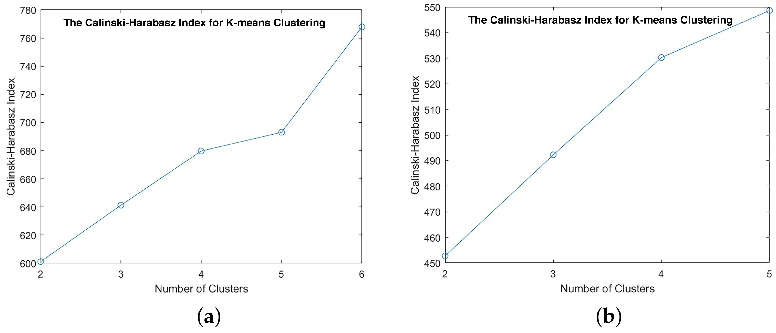
2.2. K-Means Clustering

K-means clustering is an unsupervised machine learning algorithm used for grouping data points into clusters based on similarity. The method has become a vital tool in statistical data analysis and is exploited in various disciplines, including information retrieval, pattern recognition, and machine learning. Some of the benefits of K-means clustering are its straightforward implementation, simplicity, and ability to handle large datasets with low computational complexity. The approach iteratively assigns data points to the nearest centroid based on a distance metric, commonly the Euclidean distance, and updates the centroids until convergence. The pseudocode of the K-means clustering algorithm is presented in Algorithm 2.

Algorithm 2 K-means clustering algorithm

Input: dataset of points $X=\left\{x_1,\dots ,x_n\right\}$;           number of clusters k

Output: k clusters $C_1,\dots ,C_k$ with its centroid $c_1,\dots ,c_k$ 1: repeat 2:     randomly initialize k centroid $c_1,\dots ,c_k$ 3:     for $i=1$ to n do 4:         for $j=1$ to k do 5:            assign $x_i$ to closest centroid: 6:            if $\left|\right|x_i-c_j\left|\right|<\left|\right|x_i-c_l\left|\right|$, $j\ne l$ and $1\le j,l\le k$ then 7:                $C_j=C_j\cup \left\{x_i\right\}$ 8:            end if 9:         end for 10:     end for 11:     for $j=1$ to k do 12:         centroid update $c_j=\frac{1}{|C_j|}{\sum }_{x\in C_j}x$ 13:     end for 14: until stopping criteria is met

In the process of clustering, an essential initial step is identifying the number of clusters, k. Several techniques of cluster number selection have been put forward, such as the elbow method [34], the silhouette index [35], the Calinski-Harabasz index [36], and the gap statistics [37].

This study uses the Calinski-Harabasz index or variance ratio criterion to determine the optimal number of clusters. It is defined as the ratio between the group sum of squares (BGSS) and the within-group sum of squares (WGSS). To obtain well-separated and compact clusters, BGSS is maximized and WGSS is minimized. Therefore, the suitable k number of clusters is indicated by the maximum value for Calinski-Harabasz. The BGSS and WGSS are defined as

$$\mathrm{BGSS}=\sum _{j=1}^k{n}_j\left|\right|c_j-c{\left|\right|}^2,$$

(8)

$$\mathrm{WGSS}=\sum _{j=1}^k\sum _{x\in C_j}\left|\right|x-c_j{\left|\right|}^2,$$

(9)

where k is the number of clusters, $n_j$ is the number of observations in cluster j, $c_j$ is the centroid of cluster j, c is the overall mean of the data points, $C_j$ are the set of points in the cluster j, and $\left|\right|·\left|\right|$ is the Euclidean norm. The definition of Calinski-Harabasz index (CH) is given as

$$\mathrm{CH}\left(k\right)=\frac{\mathrm{BGSS}}{\mathrm{WGSS}}\times \frac{n-k}{k-1},$$

(10)

where n is the number of observations.

3. Methodology

In this section, we develop a novel window selection approach for moving window kriging in which the clusters are quantitatively classified through the K-means clustering technique. We start by covering a background of moving window kriging and then window selection based on K-means clustering.

3.1. Moving Window Kriging

Moving window kriging is an extension of the traditional kriging methods, which allows for a localized estimation of values at target points. Its concept is to first define a window or neighborhood around each target point. The available data points inside this specified window are thereafter used to estimate the unknown quantities within the framework of kriging algorithms. In particular, OK is employed in this study. Algorithm 3 for the moving window kriging involves the following steps:

Algorithm 3 Moving window kriging algorithm

Input: observed data $Z\left(x_1\right),Z\left(x_2\right),\dots ,Z\left(x_n\right)$ at positions $x_1,x_2,\dots ,x_n$;           target points $x_{0i}$ for $i=1,2,\dots ,p$

Output: estimated values $\widehat{Z}\left(x_{0i}\right)$ of $Z\left(x_{0i}\right)$ at the target points $x_{0i}$ for $i=1,2,\dots ,p$ 1: for$i=1$ to p do 2:     define a window of $x_{0i}$, $W_{0i}$ 3:     identify the positions of observed data situated inside the window $W_{0i}$ 4:     apply the OK algorithm within the window $W_{0i}$ to obtain estimated value $\widehat{Z}\left(x_{0i}\right)$ 5: end for

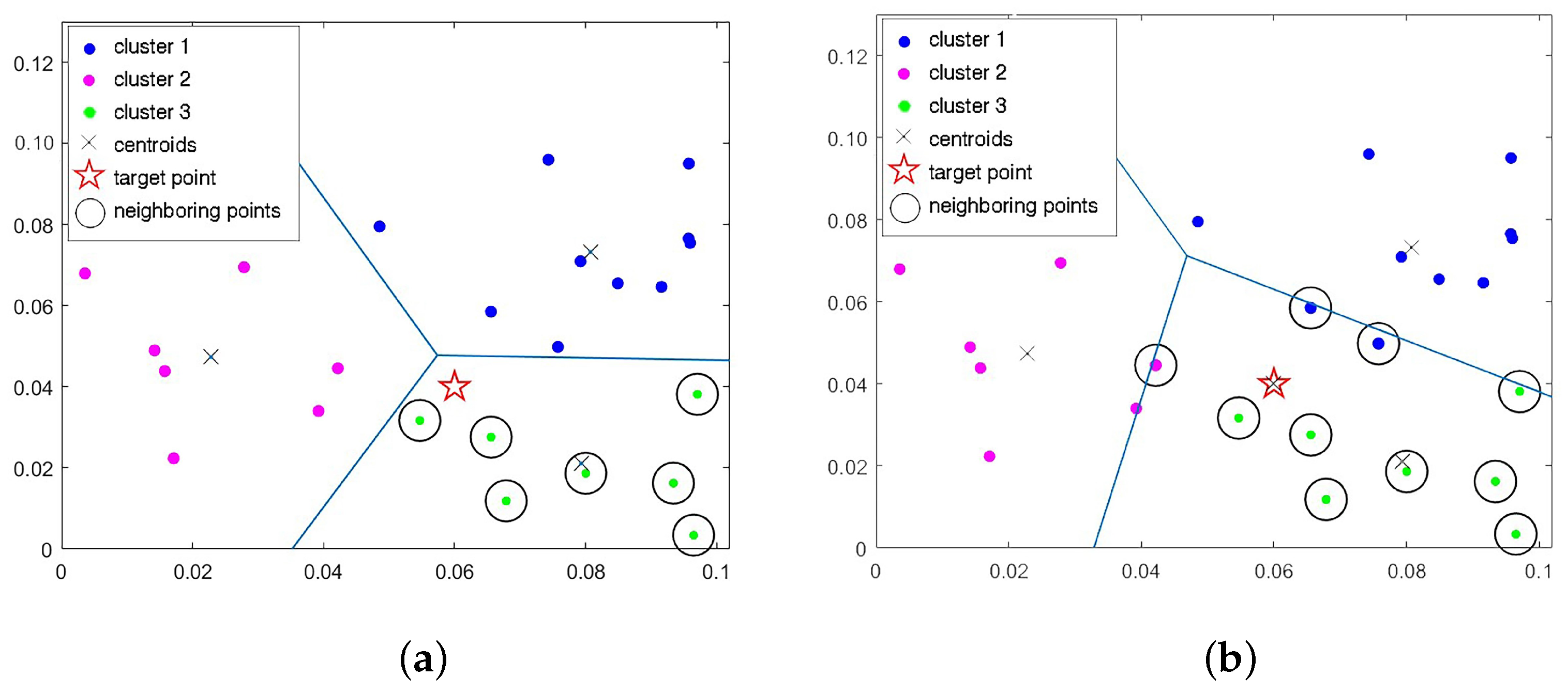
3.2. Window Selection Based on K-Means Clustering

The process of choosing a window member is of the utmost importance in the context of kriging with movable windows. Numerous factors demand careful consideration during the selection of a window. Nevertheless, there are no precise recommendations for determining the appropriate window for the moving window kriging interpolation method with different data sets. This work arose from the need to solve this practical problem. By integrating K-means clustering into the window selection process of moving window kriging, we aimed to enhance the accuracy and efficiency of spatial interpolation.

Let $Z\left(x_1\right),Z\left(x_2\right),\dots ,Z\left(x_n\right)$ be the observations at n different positions $x_1,x_2,\dots ,x_n$ in the spatial domain D. Let $x_{0i}$ for $i=1,2,\dots ,p$ be target positions, which in this study is defined as $x_{0i}=({\lambda }_{x_{0i}},{\varphi }_{x_{0i}})$, where ${\lambda }_{x_{0i}}$ is the longitude and ${\varphi }_{x_{0i}}$ is the latitude at the ith target point. The objective of the present work, known as Adaptive Moving Window Kriging using K-means Clustering (AMWKK), is to improve the cluster-based kriging introduced by Abedini et al. Instead of using centroids in a fixed manner throughout the simulation, each target site served as a cluster centroid, leading to a new set of clusters being sequentially formed. The moving window ordinary kriging method then proceeds within a cluster where the target point is located. The outline of AMWKK method for assigning appropriate neighboring points based on K-means clustering in the context of moving window ordinary kriging is presented in Algorithm 4.

Algorithm 4 Window selection based on the K-means clustering algorithm

Input: sampling positions $X=\left\{x_1,\dots ,x_n\right\}$;           number of clusters k;           target points $x_{0i}$ for $i=1,2,\dots ,p$

Output: windows $W_{0i}$ of the points $x_{0i}$ for $i=1,2,\dots ,p$ 1: apply K-means algorithm to obtain k clusters $C_1,\dots ,C_k$ with the set of its centroids $c=\left\{c_1,\dots ,c_k\right\}$ 2: for $i=1$ to p do 3:     if $x_{0i}\in C_m$ for some $m\in \left\{1,2,\dots ,k\right\}$ then 4:         $c_m=x_{0i}$ 5:         $c=\left\{c_1,\dots ,c_{m-1},x_{0i},c_{m+1},\dots ,c_k\right\}$ 6:     end if 7:     for $q=1$ to n do 8:         for $j=1$ to k do 9:            assign $x_j$ to closest centroid: 10:            if $\left|\right|x_q-c_j\left|\right|<\left|\right|x_q-c_l\left|\right|$, $j\ne l$ and $1\le j,l\le k$ then 11:                $C_j=C_j\cup \left\{x_q\right\}$ 12:            end if 13:         end for 14:     end for 15:     $W_{0i}=C_m$ 16: end for

Figure 1 depicts the conceptual difference in window selection between the Abedini et al. technique and the AMWKK approach. A pragmatic issue regarding the cluster-based kriging of Abedini et al. can be seen in Figure 1a when the target point, denoted by a star, is situated near the cluster borders. More specifically, the target point is in cluster 3, and all data belonging to this cluster are required for the estimation. However, there are points near the borders that reside in other clusters and are closer to the target point than some cluster 3 members. An adaptation of AMWKK is to select the target point to be a new centroid for the cluster instead, as shown in Figure 1b. This allows for more suitable observed data that has similar characteristics to the target point to be included through the K-means clustering algorithm.

4. Case Study: Spatial Interpolation of Meteorological Data in Thailand

4.1. Data Description

The study area is located in Thailand ($5^{°}{37}^{\prime }$ N to ${20}^{°}{27}^{\prime }$ N, ${97}^{°}{22}^{\prime }$ E to ${105}^{°}{37}^{\prime }$ E), which covers an area of 518,000 ${\mathrm{km}}^2$. The data used in this study consist of annual averages of pressure, relative humidity, and geographic locations (coordinates). The hourly data were collected from the National Hydroinformatics and Climate Data Center (NHC), developed by the Hydro-Informatics Institute (HII) over an observed period spanning from January 2018 to December 2018 [38]. Each dataset was attained from 930 meteorological stations. After identifying and eliminating the outlier samples, we used hourly averages of the remaining 318 pressure and 239 humidity data. The positions for each of the two datasets are shown in Figure 2.

4.2. Accuracy Assessment

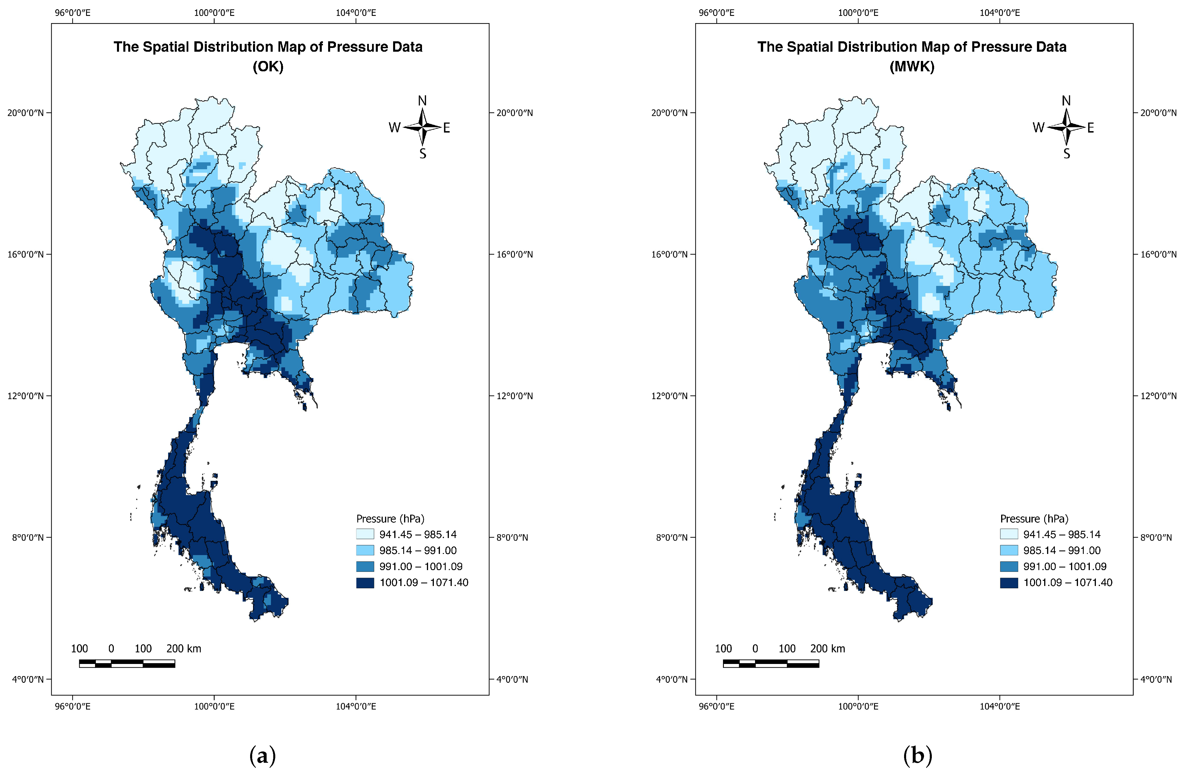
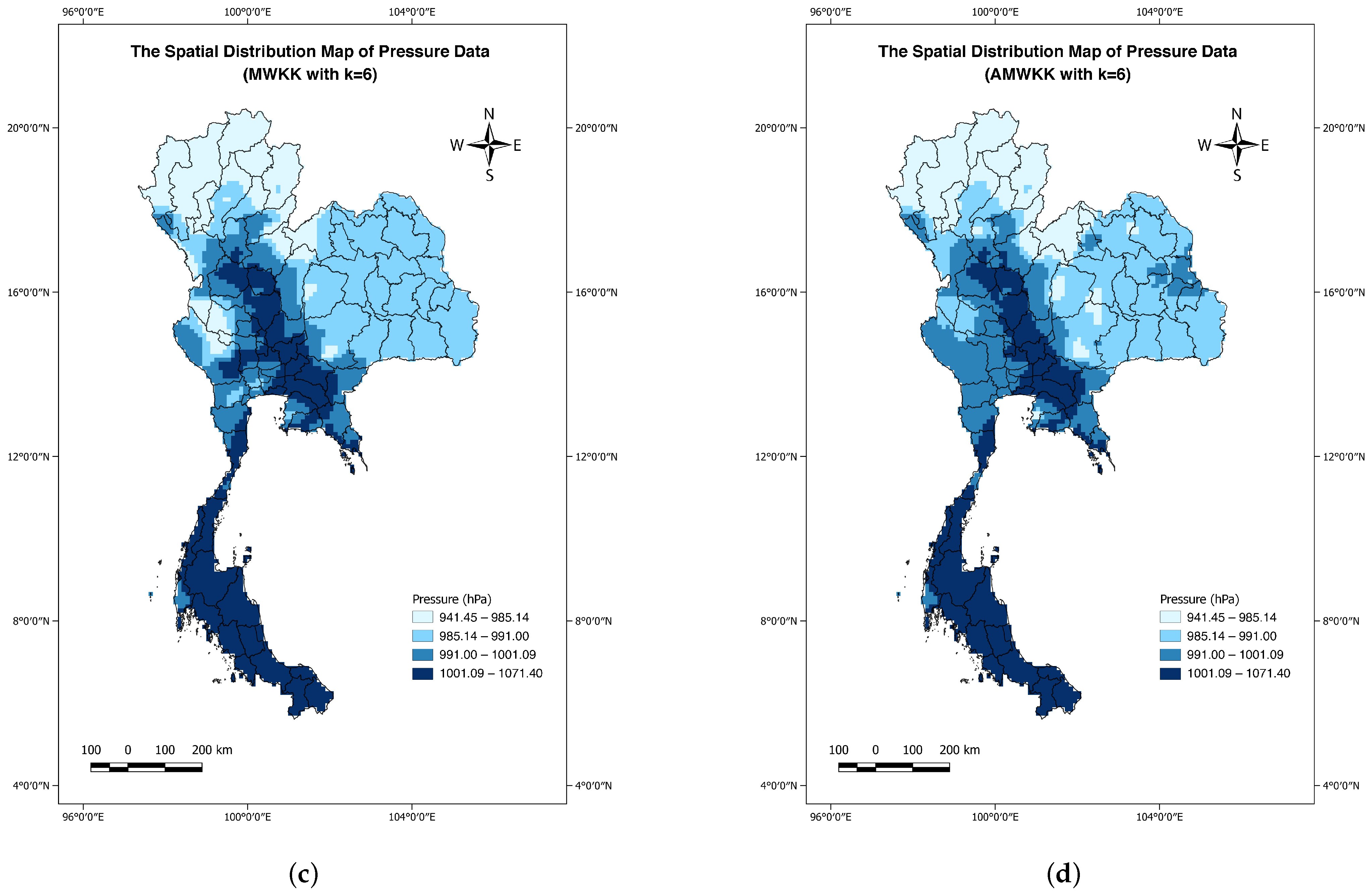
For model validation, we used the k-fold cross-validation technique, in which the data were partitioned into 10 folds of approximately equal size. Each fold was selected once for testing the model induced from the remaining nine subsets. The process was repeated 10 times until every fold was used as the testing dataset. The overall model performance was subsequently evaluated by averaging the 10 errors.

Our work compared three main kriging models: OK, moving window kriging with a fixed window size, and adaptive moving window kriging using the K-means clustering algorithm (AMWKK). In addition, two different criteria for selecting a window size for the moving window kriging were carried out, namely, the fixed prescribed number (30 positions) (MWK) and the K-means clustering algorithm (MWKK). To assess the estimation ability of each model, we computed distinct quantitative performance metrics, including the mean absolute percentage error (MAPE), root mean square error (RMSE), percentage average estimation error (PAEE), and normalized mean squared error (NMSE). They are formulated as follows:

$$\mathrm{MAPE}=\frac{1}{n}\sum _{i=1}^n\left|\frac{Z\left(x_i\right)-\widehat{Z}\left(x_i\right)}{Z\left(x_i\right)}\right|\times 100,$$

(11)

$$\mathrm{RMSE}=\sqrt{\frac{1}{n}\sum _{i=1}^n{(Z\left(x_i\right)-\widehat{Z}\left(x_i\right))}^2},$$

(12)

$$\mathrm{PAEE}=\frac{1}{n\overline{Z}}\sum _{i=1}^n\left|Z\left(x_i\right)-\widehat{Z}\left(x_i\right)\right|,$$

(13)

$$\mathrm{NMSE}=\frac{1}{n{s}^2}\sum _{i=1}^n{\left(Z\left(x_i\right)-\widehat{Z}\left(x_i\right)\right)}^2,$$

(14)

where n is the number of observations, and $Z\left(x_i\right)$ and $\widehat{Z}\left(x_i\right)$ represent the actual measured data and the estimated value at position $x_i$, respectively. $\overline{Z}$ is the average and $s^2$ is the variance of the actual measured data.

A relative improvement (${\mathrm{R}}_{\mathrm{I}}$) regarding RMSE values of moving window kriging variants over the ordinary kriging model was also exploited as another measure for accuracy evaluation, and is defined as

$${\mathrm{R}}_{\mathrm{I}}=\frac{{\mathrm{RMSE}}_{\mathrm{OK}}-\mathrm{RMSE}}{{\mathrm{RMSE}}_{\mathrm{OK}}}\times 100\%.$$

(15)

4.3. Results

The simulations were conducted using MATLAB software (version 2018a) to assess the performances of all four algorithms. Prior to the MWKK and AMWKK implementations, a predetermination of a suitable k clustering number in the K-means algorithm is required. Here, we computed the Calinski–Harabasz index to indicate the optimal k number of clusters. With the lowest number of neighboring positions suggested by Journel and Huijbregts [3] being 30 positions, the possible number k of K-means clusters for both MWKK and AMWKK approaches was thereby in the range of 2 to 6 for pressure and 2 to 5 for humidity. According to Figure 3a,b, the value of Calinski–Harabasz index increased as the number of clusters increased. The optimal numbers of clusters corresponding to the maximum Calinski–Harabasz index were 6 and 5 for pressure and humidity, respectively.

Table 1. Performance of different interpolation methods for annual pressure data in 2018.

Interpolation Method	Mean MAPE (%)	Mean RMSE	Mean PAEE	Mean NMSE	${\mathbf{R}}_{\mathbf{I}}$ (%)
OK	1.0243	14.7254	0.0101	0.6393	-
MWK	0.9910	14.4277	0.0098	0.6176	2.0218
MWKK with k = 6	0.9841	14.5030	0.0097	0.6238	1.5102
AMWKK with k = 6	0.9822	14.3834	0.0097	0.6128	2.3226

displays the pressure estimation efficiency of all of the models. Regarding diagnostic statistics, all moving window kriging variants had superior estimation performances compared with the benchmark OK model. In particular, the mean MAPE and PAEE values of the OK model were above 1.000 and 0.0100, in contrast with those of the others whose error values were below these values. The results from the moving window kriging showed a comparable improvement in which AMWKK yielded the best estimation with an improvement equal to 2.3226% relative to the OK model.

A similar trend of results was observed in the case of humidity, as shown in

Table 2. Performance of different interpolation methods for annual humidity data in 2018.

Interpolation Method	Mean MAPE (%)	Mean RMSE	Mean PAEE	Mean NMSE	${\mathbf{R}}_{\mathbf{I}}$ (%)
OK	2.2915	2.2028	0.0229	0.5170	-
MWK	2.1813	2.1124	0.0218	0.4770	4.1040
MWKK with k = 5	2.2087	2.1217	0.0220	0.4833	3.6795
AMWKK with k = 5	2.1672	2.0804	0.0216	0.4641	5.5571

. The moving window kriging approaches continued to outperform the OK method, with relative RMSE improvements between 3.6795% and 5.5571%. When comparing the moving window krigings, the AMWKK method exhibited better results than the MWK and MWKK techniques, with the estimation quality regarding NMSE statistics being improved by 2.7044% and 3.9727%, respectively.

The results from both cases indicate that the improvement in the moving window kriging was achieved by exploiting the moving centroids. To further investigate the estimation effectiveness of all methods, we present the spatial distributions of Thailand’s averages hourly pressure and humidity in 2018. The study area was systematically divided into square cells measuring 0.25 degrees per side, roughly equivalent to 5.5 square kilometers each. After the longitude and latitude of the grid center point were identified, the pressure and humidity values were then estimated using all four methods at these locations. The spatial distribution maps of the estimation results were created using the QGIS software (Version 3.34.0) [39,40,41,42,43].

The spatial interpolation maps for annual averages from hourly pressure are displayed in Figure 4. The pressure values ranged from 941.45 to 1071.40 hPa. The lowest pressure value (941.45 hPa) was found in the north, while the highest (1071.40 hPa) was in the south. Since forested mountains are the main geographical features of the northern and northeastern regions, lower pressure is observed in these areas. Conversely, the central and southern parts resembled flat areas, reflecting higher pressure levels. It was observed that pressure increased from north to south as altitude decreased and geographical features were taken into account.

A difference in pressure distribution obtained from OK and the moving kriging variants was identified in the southern region, where lower pressure levels were broadly distributed using OK. In the central region, the high-pressure intensity (1001.09–1071.40 hPa) achieved from the OK model was more widely spread than those of the AMWKK, MWKK, and MWK estimates. Meanwhile, all moving window kriging methods generated a few distinct pressure values across the region. The MWK and AMWKK methods exhibited a similar distribution pattern, except in the central region. This also supported the results in Table 1, where the most effective performance was achieved by the AMWKK model, followed by MWK.

The spatial distribution maps for the annual average of hourly relative humidity are plotted in Figure 5, with the minimum value being 70.80% in the northeast and the highest value being 82.25% in the southernmost part of the study area. In every spatial model we obtained, the southern part of the study area always had a high relative humidity, as the values changed based on their distance from the ocean. This spatial distribution map was consistent with the relative humidity pattern, which indicates that the low values in northeast Thailand were connected to the arid climatic zones, while the southern areas directly adjacent to the sea coast had high relative humidity levels. Similar to pressure, the OK interpolation provided a different distribution pattern from other moving window kriging models, especially in northeastern Thailand, where relative humidity had high-value dispersion in some areas. Meanwhile, the MWK and AMWKK methods produced indistinct geographical predictions with similar distribution maps. This corresponded to the results in Table 2, in which the AMWKK provided the best estimation performance, and MWK the second best, respectively.

5. Discussion

Despite satisfactory quantitative results in the case study, there is still room for improvement in the model efficiency. The performance of the K-means clustering algorithm relies on various factors: the suitable number of clusters k, an outlier sensitivity problem, and a selection of initial centroids. If there are many clusters, only a few data points are situated in each cluster, leading to erratic variograms. On the other hand, for a small number of k, spurious correlation can affect the model prediction. Identification of the minimum number of cluster elements is additionally required to capture spatial variability. Furthermore, outliers can cause a misspecification of cluster centroids, causing less reliable results. In this work, data preprocessing was carried out to eliminate outliers. Additionally, the Calinski–Harabasz index was also employed to ascertain the optimal number of clusters. However, the suitability of this approach may be contingent upon the specific characteristics of the data and the research objectives. Alternative methods, such as the gap statistics, the silhouette index, and the density canopy algorithm [44], could offer valuable insights and potentially yield different results. Last, but most importantly, the time complexity of OK is typically $O\left(n^3\right)$ [45,46,47] where n is the number of data points, whereas that of our algorithm depends on two processes: the ordinary kriging and the K-means clustering system. The computational complexity of the K-means algorithm is $O\left(nkt\right)$ [48,49,50] where t is the number of iterations. To mitigate such issues, some effective algorithms that can find appropriate initial centroids can simultaneously reduce the number of k and t, resulting in a reduction in computational cost. The proposed window selection algorithm is not limited to the OK model. However, it could be applied to broader ranges of kriging models that incorporate auxiliary variables influencing the target variable via the trend function, such as regression kriging (RK) and kriging with external drift (KED) [51,52]. These techniques specifically operate on a subset of data confined within the selected window for the estimation.

6. Conclusions

In this work, the AMWKK method is developed to improve the spatial prediction derived from the moving window kriging based on the K-means clustering proposed by Abedini et al. Unlike the MWK method (Journel and Huijbregts [3]) and MWKK method (Abedini et al. [29]), which employ fixed window sizes and fixed centroids, respectively, the AMWKK model utilizes a dynamic clustering approach. Here, each target site acts as a temporary cluster centroid, which initiates the formation of new clusters. These clusters serve as the window for estimating the target point’s value. This technique specifically addresses the challenge of selecting appropriate windows for target points located near the borders, which can potentially be the source of errors. This novel approach offers a computationally efficient alternative to cross-validation for window size selection presented by Fotheringham et al. [26] and Haas [20,27]. AMWKK and other interpolation approaches are used to estimate Thailand’s mean annual pressure and humidity in 2018. The results indicate the superior estimation capabilities of the AMWKK approach, with ${\mathrm{R}}_{\mathrm{I}}$ values of 2.3226% and 5.5571% for the pressure and humidity, respectively. In this regard, the advantage of using the AMWKK method for spatial interpolation can be attributed to the fact that it facilitates the automatic tuning of the window size at any estimation point, which is particularly effective when observations in the same cluster as target points are sparse.

References

1. Krige, D.G. A statistical approach to some basic mine valuation problems on the Witwatersrand. J. S. Afr. Inst. Min. Metall. 1951, 52, 119–139. [Google Scholar]
2. Matheron, G. Principles of geostatistics. Econ. Geol. 1963, 58, 1246–1266. [Google Scholar] [CrossRef]
3. Journel, A.G.; Huijbregts, C.J. Mining Geostatistics; Academic Press: London, UK, 1978. [Google Scholar]
4. Lamamra, A.; Neguritsa, D.L.; Mazari, M. Geostatistical modeling by the Ordinary Kriging in the estimation of mineral resources on the Kieselguhr mine, Algeria. In IOP Conference Series: Earth and Environmental Science; IOP Publishing: Bristol, UK, 2019; Volume 362, p. 012051. [Google Scholar]
5. Singh, R.K.; Ray, D.; Sarkar, B. Mineral deposit grade assessment using a hybrid model of kriging and generalized regression neural network. Neural Comput. Appl. 2022, 34, 10611–10627. [Google Scholar] [CrossRef]
6. Schorr, J.; Cudmani, R.; Nübel, K. Interpretation of field tests using geo-statistics and Kriging to assess the deep vibratory compaction of the Dike A21, Diavik Diamond Mine. Acta Geotech. 2023, 18, 1391–1405. [Google Scholar] [CrossRef]
7. Kingsley, J.; Lawani, S.O.; Esther, A.O.; Ndiye, K.M.; Sunday, O.J.; Penížek, V. Predictive mapping of soil properties for precision agriculture using geographic information system (GIS) based geostatistics models. Mod. Appl. Sci. 2019, 13, 60–77. [Google Scholar] [CrossRef]
8. Aryafar, A.; Khosravi, V.; Karami, S. Groundwater quality assessment of Birjand plain aquifer using kriging estimation and sequential Gaussian simulation methods. Environ. Earth Sci. 2020, 79, 210. [Google Scholar] [CrossRef]
9. Munyati, C.; Sinthumule, N. Comparative suitability of ordinary kriging and Inverse Distance Weighted interpolation for indicating intactness gradients on threatened savannah woodland and forest stands. Environ. Sustain. Indic. 2021, 12, 100151. [Google Scholar] [CrossRef]
10. Dai, H.; Huang, G.; Wang, J.; Zeng, H.; Zhou, F. Spatio-Temporal Characteristics of PM2.5 Concentrations in China Based on Multiple Sources of Data and LUR-GBM during 2016–2021. Int. J. Environ. Res. Public Health 2022, 19, 6292. [Google Scholar] [CrossRef]
11. Zhang, Z.; Du, Q. A bayesian kriging regression method to estimate air temperature using remote sensing data. Remote Sens. 2019, 11, 767. [Google Scholar] [CrossRef]
12. Zhang, G.; Tian, G.; Cai, D.; Bai, R.; Tong, J. Merging radar and rain gauge data by using spatial–temporal local weighted linear regression kriging for quantitative precipitation estimation. J. Hydrol. 2021, 601, 126612. [Google Scholar] [CrossRef]
13. Das, S.; Islam, A.R.M.T. Assessment of mapping of annual average rainfall in a tropical country like Bangladesh: Remotely sensed output vs. kriging estimate. Theor. Appl. Climatol. 2021, 146, 111–123. [Google Scholar] [CrossRef]
14. He, Q.; Zhang, K.; Wu, S.; Lian, D.; Li, L.; Shen, Z.; Wan, M.; Li, L.; Wang, R.; Fu, E.; et al. An investigation of atmospheric temperature and pressure using an improved spatio-temporal Kriging model for sensing GNSS-derived precipitable water vapor. Spat. Stat. 2022, 51, 100664. [Google Scholar] [CrossRef]
15. Cressie, N. Spatial prediction and ordinary kriging. Math. Geol. 1988, 20, 405–421. [Google Scholar] [CrossRef]
16. Wackernagel, H. Multivariate Geostatistics: An Introduction with Applications; Springer Science & Business Media: New York, NY, USA, 2003. [Google Scholar]
17. Chiles, J.P.; Delfiner, P. Geostatistics: Modeling Spatial Uncertainty; John Wiley and Sons: Hoboken, NJ, USA, 2012; Volume 713. [Google Scholar]
18. Tan, Q.; Xu, X. Comparative analysis of spatial interpolation methods: An experimental study. Sens. Transducers 2014, 165, 155. [Google Scholar]
19. Marwanza, I.; Nas, C.; Azizi, M.; Simamora, J. Comparison between moving windows statistical method and kriging method in coal resource estimation. In Journal of Physics: Conference Series; IOP Publishing: Bristol, UK, 2019; Volume 1402, p. 033016. [Google Scholar]
20. Haas, T.C. Kriging and automated variogram modeling within a moving window. Atmos. Environ. Part A 1990, 24, 1759–1769. [Google Scholar] [CrossRef]
21. Alkhaled, A.A.; Michalak, A.M.; Kawa, S.R.; Olsen, S.C.; Wang, J.W. A global evaluation of the regional spatial variability of column integrated CO2 distributions. J. Geophys. Res. Atmos. 2008, 113. [Google Scholar] [CrossRef]
22. Hammerling, D.M.; Michalak, A.M.; Kawa, S.R. Mapping of CO2 at high spatiotemporal resolution using satellite observations: Global distributions from OCO-2. J. Geophys. Res. Atmos. 2012, 117, D06306. [Google Scholar] [CrossRef]
23. Haas, T.C. Multivariate spatial prediction in the presence of non-linear trend and covariance non-stationarity. Environmetrics 1996, 7, 145–165. [Google Scholar] [CrossRef]
24. Lloyd, C.D.; Atkinson, P.M. Non-stationary approaches for mapping terrain and assessing prediction uncertainty. Trans. GIS 2002, 6, 17–30. [Google Scholar] [CrossRef]
25. Pardo-Igúzquiza, E.; Dowd, P.A.; Grimes, D.I. An automatic moving window approach for mapping meteorological data. Int. J. Climatol. 2005, 25, 665–678. [Google Scholar] [CrossRef]
26. Fotheringham, A.S.; Brunsdon, C.; Charlton, M. Geographically Weighted Regression: The Analysis of Spatially Varying Relationships; John Wiley & Sons: Chichester, UK, 2003. [Google Scholar]
27. Haas, T.C. Local prediction of a spatio-temporal process with an application to wet sulfate deposition. J. Am. Stat. Assoc. 1995, 90, 1189–1199. [Google Scholar] [CrossRef]
28. Van Stein, B.; Wang, H.; Kowalczyk, W.; Emmerich, M.; Bäck, T. Cluster-based Kriging approximation algorithms for complexity reduction. Appl. Intell. 2020, 50, 778–791. [Google Scholar] [CrossRef]
29. Abedini, M.; Nasseri, M.; Ansari, A. Cluster-based ordinary kriging of piezometric head in West Texas/New Mexico–Testing of hypothesis. J. Hydrol. 2008, 351, 360–367. [Google Scholar] [CrossRef]
30. Yasojima, C.; Protázio, J.; Meiguins, B.; Neto, N.; Morais, J. A new methodology for automatic cluster-based kriging using K-nearest neighbor and genetic algorithms. Information 2019, 10, 357. [Google Scholar] [CrossRef]
31. Cressie, N.; Hawkins, D.M. Robust estimation of the variogram: I. J. Int. Assoc. Math. Geol. 1980, 12, 115–125. [Google Scholar] [CrossRef]
32. Cressie, N. Statistics for Spatial Data; John Wiley & Sons: New York, NY, USA, 1993. [Google Scholar]
33. Cressie, N. Fitting variogram models by weighted least squares. J. Int. Assoc. Math. Geol. 1985, 17, 563–586. [Google Scholar] [CrossRef]
34. Syakur, M.; Khotimah, B.; Rochman, E.; Satoto, B.D. Integration k-means clustering method and elbow method for identification of the best customer profile cluster. In IOP Conference Series: Materials Science and Engineering; IOP Publishing: Bristol, UK, 2018; Volume 336, p. 012017. [Google Scholar]
35. Rousseeuw, P.J. Silhouettes: A graphical aid to the interpretation and validation of cluster analysis. J. Comput. Appl. Math. 1987, 20, 53–65. [Google Scholar] [CrossRef]
36. Caliński, T.; Harabasz, J. A dendrite method for cluster analysis. Commun. Stat. 1974, 3, 1–27. [Google Scholar]
37. Tibshirani, R.; Walther, G.; Hastie, T. Estimating the number of clusters in a data set via the gap statistic. J. R. Stat. Soc. Ser. B Stat. Methodol. 2001, 63, 411–423. [Google Scholar] [CrossRef]
38. OpenData. Available online: https://data.hii.or.th (accessed on 27 October 2020).
39. Valjarević, A.; Srećković-Batoćanin, D.; Valjarević, D.; Matović, V. A GIS-based method for analysis of a better utilization of thermal-mineral springs in the municipality of Kursumlija (Serbia). Renew. Sustain. Energy Rev. 2018, 92, 948–957. [Google Scholar] [CrossRef]
40. Valjarević, A.; Živković, D.; Gadžić, N.; Tomanović, D.; Grbić, M. Multi-criteria GIS analysis of the topography of the Moon and better solutions for potential landing. Open Astron. 2019, 28, 85–94. [Google Scholar] [CrossRef]
41. Sansare, D.A.; Mhaske, S.Y. Natural hazard assessment and mapping using remote sensing and QGIS tools for Mumbai city, India. Nat. Hazards 2020, 100, 1117–1136. [Google Scholar] [CrossRef]
42. Muller, A.; Gericke, O.; Pietersen, J. Methodological approach for the compilation of a water distribution network model using QGIS and EPANET. J. S. Afr. Inst. Civ. Eng. 2020, 62, 32–43. [Google Scholar] [CrossRef]
43. Elangovan, K.; Krishnaraaju, G. Mapping and Prediction of Urban Growth using Remote Sensing, Geographic Information System, and Statistical Techniques for Tiruppur Region, Tamil Nadu, India. J. Indian Soc. Remote Sens. 2023, 51, 1657–1671. [Google Scholar] [CrossRef]
44. Geng, Z.; Chengchang, Z.; Huayu, Z. Improved K-means Algorithm Based on Density Canopy. Knowl.-Based Syst. 2018, 145, 289–297. [Google Scholar]
45. Zhong, X.; Kealy, A.; Duckham, M. Stream Kriging: Incremental and recursive ordinary Kriging over spatiotemporal data streams. Comput. Geosci. 2016, 90, 134–143. [Google Scholar] [CrossRef]
46. Memarsadeghi, N.; Raykar, V.C.; Duraiswami, R.; Mount, D.M. Efficient kriging via fast matrix-vector products. In Proceedings of the 2008 IEEE Aerospace Conference, Big Sky, MT, USA, 1–8 March 2008; pp. 1–7. [Google Scholar]
47. Vlastos, P.G.; Hunter, A.; Curry, R.; Ramirez, C.I.E.; Elkaim, G. Partitioned gaussian process regression for online trajectory planning for autonomous vehicles. In Proceedings of the 2021 21st International Conference on Control, Automation and Systems (ICCAS), Jeju, Republic of Korea, 12–15 October 2021; IEEE: New York, NY, USA, 2021; pp. 1160–1165. [Google Scholar]
48. Kushwaha, M.; Yadav, H.; Agrawal, C. A review on enhancement to standard k-means clustering. In Social Networking and Computational Intelligence: Proceedings of SCI-2018; Springer: Heidelberg, Germany, 2020; pp. 313–326. [Google Scholar]
49. Fahim, A.M. An Efficient Parallel K-Means On Multi-Core Processors. Int. J. Sci. Eng. Technol. Res. (IJSETR) 2015, 4, 4234–4241. [Google Scholar]
50. Peng, C.; Guiqiong, X. A brief study on clustering methods: Based on the k-means algorithm. In Proceedings of the 2011 International Conference on E-Business and E-Government (ICEE), Shanghai, China, 6–8 May 2011; IEEE: New York, NY, USA, 2011; pp. 1–5. [Google Scholar]
51. Hengl, T.; Heuvelink, G.B.; Stein, A. Comparison of Kriging with External Drift and Regression Kriging; ITC Enschede: Enschede, The Netherlands, 2003. [Google Scholar]
52. Hengl, T.; Heuvelink, G.B.; Rossiter, D.G. About regression-kriging: From equations to case studies. Comput. Geosci. 2007, 33, 1301–1315. [Google Scholar] [CrossRef]
Figure 1. Example of the difference of window selection between the original K-means algorithm and the AMWKK approach with three clusters: (a) K-means clustering data with k = 3 and (b) Adaptive K-means clustering data with k = 3 .
Algorithms 17 00057 g001
Figure 2. Positions of the study area for meteorological data in 2018: (a) pressure (blue points) and (b) humidity (green points).
Algorithms 17 00057 g002
Figure 3. The Calinski–Harabasz index of K-means clustering: (a) pressure and (b) humidity data.
Algorithms 17 00057 g003
Figure 4. The annual pressure kriging estimate maps using the different spatial interpolation methods: (a) OK, (b) MWK, (c) MWKK with k = 6 , and (d) AMWKK with k = 6 .
Algorithms 17 00057 g004aAlgorithms 17 00057 g004b
Figure 5. The annual humidity kriging estimate maps using the different spatial interpolation methods: (a) OK, (b) MWK, (c) MWKK with k = 5 , and (d) AMWKK with k = 5 .
Algorithms 17 00057 g005