Abstract
In this paper, we recover the European option volatility function of the underlying asset and the fractional order of the time fractional derivatives under the time fractional Vasicek model. To address the ill-posed nature of the inverse problem, we employ Tikhonov regularization. The Alternating Direction Multiplier Method (ADMM) is utilized for the simultaneous recovery of the parameter and the volatility function . In addition, the existence of a solution to the minimization problem has been demonstrated. Finally, the effectiveness of the proposed approach is verified through numerical simulation and empirical analysis.
1. Introduction
The option pricing problem is an important issue in the financial field. Black and Scholes [1] introduced the Black–Scholes (BS) formula, assuming a constant risk-free rate r and that the underlying asset S satisfies the following equation
where is the expected return rate, is the volatility, and is the standard Brown motion. Under these conditions, the BS formula is derived as
where
denotes the cumulative standard normal distribution function, and K is the exercise price. However, in real financial markets, interest rates change over time. Therefore, in the option pricing process, the impact of interest rate uncertainty on option prices must be considered. There are various interest rate models, including the Constant Elasticity of Variance (CEV) model [2], Cox–Ingersoll–Ross (CIR) model [3], Vasicek model [4], etc. Specifically, our focus in this article is on the Vasicek model.
Fractional derivatives are widely used in fractal theory [5], diffusion theory [6], signal processing [7], and financial theory ([8,9,10]) due to their non-locality advantages, i.e., the current state is influenced not only by the past instantaneous state but also by the state of the past period of time, which is more in line with the options market. Fractional derivative have two main forms: the Riemann–Liouville derivative [11] and the Caputo derivative [12]. In our discussion, we are mainly concerned with fractional derivatives in the Caputo sense. Since most partial differential equations lack analytic solutions, discretization of the equations in time and space is necessary. The commonly used methods for discrete Caputo time fractional derivatives include the Grnwald–Letnikov (GL) formula and L1 formula. Specifically, the GL formula has a first-order accuracy in time direction after discretization, while the L1 formula has a (2-)-order accuracy in time direction. Subsequently, Gao et al. [13] introduced the L1-2 formula with (3-)-order accuracy, Alikhanov [14] proposed the L2- formula with (3-)-order accuracy, and Cao et al. [15] improved the accuracy of the discretization to the (3-)-order Caputo derivative. In recent studies, Cao et al. [16] and Mokhtari et al. [17] improved the accuracy to (4-)-order. It is worth noting that the process of improving accuracy involves a higher-order interpolation of the function under the integral of the Caputo derivative. Using different interpolation functions results in different levels of precision.
Nourian et al. [8] solved the time fractional Black–Scholes equation by introducing a new set of wavelet functions. Roul [9] constructed a high-order computational scheme for European option pricing; this method is (3-)-order in the time direction. Chen et al. [10] introduced a novel operator splitting method to address American options within the framework of the time-fractional Black–Scholes model. Li et al. [18] presented a Newton-linearized Galerkin finite element method for solving time-oriented nonsmooth nonlinear time-fraction parabolic problems. The optimal error estimate of L2 norm is obtained without limitation of time step of spatial mesh size. The theoretical results are verified by numerical experiments. In [19], the convergence of a class of fully implicit time-stepping Galerkin finite element method for one-dimensional nonlinear subdiffusion equations is proved by using the generalized discrete Gronwall inequality. Based on the convergence of the direct time step scheme, a simple method to prove the convergence of the fast time-stepping Galerkin finite element method is presented. Yuan et al. [20] proposed a linearized fast high-order time-stepping scheme to solve the spatiotemporal fractional Schrodinger equation. A fast L2- formula was used to approximate the time of non-uniform mesh. The Fourier spectrum method is used to discretize the space. The result of unconditional convergence is given. Zhang and Jiang [21] considered the two-dimensional nonlinear time-space fractional Schrodinger equation and applied the second-order fractional backward difference formula in the time direction and the Fourier spectrum method in the space direction to solve the model numerically. By using the generalized discrete Gronwall inequality and the space-time error splitting argument, the convergence of the fast time-step numerical method is simply proved without applying the Courant–Friedrichs–Lewy (CFL) condition.
Parameter calibration is a challenging problem in the financial field. Different from the forward problem of solving option prices with known model parameters, the parameter calibration problem refers to solving the model parameters based on the price data observed in the market. The volatility is one of the most important parameters in the option pricing, which is an indicator to measure the uncertainty of the return rate of assets and is used to reflect the risk level of financial assets. However, the volatility cannot be derived directly from market data and needs to be calibrated. This is a typical inverse problem, and it is usually ill-posed because the calibration problem may have no solution or have infinite solutions, or there may be solutions that are discontinuously dependent on observation data; many scholars have conducted research in this area. Dupire [22] proposed a local volatility model for option pricing in 1994, calibrated the volatility, and obtained an expression for volatility, which is called the Dupire formula. Xu and Jia [23] studied the Tikhonov regularization method for the volatility calibration problem under the jump diffusion model and used an iterative algorithm to solve the problem to obtain the volatility. Jiang et al. [24] reconstructed the implicit local volatility function using the optimal control framework and presented numerical experiments. Based on the Legendre pseudo-spectral method of space discretization and the finite difference method of time discretization, Li and Zhou [25] gave numerical solutions for the optimal control problem of time-fractional diffusion equations. Zhao and Xu [26] jointly recovered the mean-reversion parameter and the volatility function under the fractional Chan–Karolyi–Longstaff–Sanders (CKLS) stochastic interest rate model. At the same time, numerical experiments are presented that show the fractional CKLS model ( = 0.8451) is more suitable for SSE 50ETF than the fractional Vasicek model. Yimamu and Deng [27] investigated the inverse problem of identifying volatility in option pricing. They accomplished this problem by transforming the parabolic equation defined on an unbounded region into a degenerate parabolic equation on a bounded region through a variable substitution. The study establishes that the optimal approximate solution converges effectively to the true solution of the original problem. In our paper, we use the alternating direction multiplier method to simultaneously reconstruct fractional order and time-dependent volatility function . Numerical examples and empirical analysis demonstrate the effectiveness of this method. Our research aims to reconstruct the volatility and the fractional order in the time-fractional Vasicek model. This unique perspective, to the best of our knowledge, has not been thoroughly explored in previous studies. We aim to provide readers with a novel perspective, offering a potential reference for future studies dealing with time-fractional direct problems, and offer a valuable contribution to the field by addressing the challenges associated with the simultaneous reconstruction of the volatility and the fractional order.
The remainder of this article is organized as follows. Section 2 gives the pricing formula of European put options under the time fractional Vasicek model. Section 3 gives the existence of the solution to the minimization problem and introduces the Tikhonov regularization method and ADMM algorithm for solving the volatility and the fractional order . Section 4 combines numerical examples and empirical analysis to obtain the stability of the algorithm. Finally, Section 5 provides conclusions.
2. Pricing Formula under the Time Fractional Vasicek Model
In this section, we present some fundamental definitions for our exploration and the pricing formula of European put options under the Caputo time fractional Vasicek model, laying the foundation for the subsequent exploration and reconstruction of the volatility and the parameter .
Definition 1
(Kolmogorov [28]). Assume that the system state satisfies the stochastic differential equation
where W(t) is a Wiener process (also called Brownian motion), then the conditional mathematical expectation is the solution of the Cauchy problem (terminal value problem) of the following backward parabolic equation
Definition 2
(Feynman–Kac [28]). Let v be the conditional mathematical expectation
then it is the solution of the terminal value problem of the following backward parabolic equation
Definition 3.
The Caputo time fractional derivative is defined as follows
The pricing problem of the European option under the Vasicek model is considered. Suppose the asset price adheres to the following stochastic process
and the interest rate process satisfies
where is the volatility, and are two correlated Brown motions with and , and are constants.
Zero coupon bond is the carrier of interest rate, and we first consider the pricing of zero coupon bond. Let represent the value of zero-coupon bonds at time t. When is a stochastic process, the value of zero coupon bonds is
Therefore, from the Kolmogorov theorem and the Feynman–Kac formula, we can obtain the backward parabolic equation that the price of the zero coupon bond satisfies under the Vasicek model
Next, the pricing formula of the European put option under the Vasicek model is derived.
Lemma 1.
Proof.
Consider a portfolio , which consists of units of the underlying asset S, units of the zero coupon bond , and one option , then the value of the portfolio at time t is
Applying ’s Lemma, we obtain
To eliminate risk in this portfolio, we take
substitute it into (5), then combine Formula (3) to obtain
The no-arbitrage principle gives us
then
□
To ensure the completeness of the narrative, we first introduce the direct problem.
Replacing the term in Equation (4) that involves the integer-order derivative with the Caputo fractional-order derivative, denoted as , where order , we have
the fractional order derivative is defined as
Then, we invert the time variable as and the relationship between the Caputo derivative and the time fractional derivative given by article [29], that is, .
In this way, we obtain the pricing formula of European put options under the Caputo time fractional Vasicek model
with the conditions
Direct problem: For the given initial boundary problem, the price of the European put option can be precisely computed as long as the volatility and parameter are known. Subsequently, we can use the implicit finite difference method to numerically address this problem.
Inverse problem: Let denote the market price of an option with strike price and expiration date , where and . The inverse problem is a calibration problem, which can be formulated as finding a time-dependent volatility function and parameter such that the predicted price falls between the corresponding bid price and ask price , that is
From the above formula, the calibration problem is transformed to solve such an optimization problem:
Minimize the following error function associated with the given set of market option prices
where is the mean of the bid and ask prices.
The calibration problem can be formulated as finding the parameters that minimize the error function . However, the parameter and the volatility function are discontinuously dependent on the market price, which means that small disturbances in the market price may lead to large changes in the error function . This is an ill-posed problem, so we use regularization methods to solve it.
3. Regularization Method
In this section, we introduce the Tikhonov regularization [30,31] to make the problem well posed. We calibrate fractional order and volatility function by minimizing the following optimization problem
where , represents -norm, is the regularization parameter, and is the real market option price.
3.1. Existence of Solutions to Optimization Problems
In the following theorem, we establish the existence of a solution to the minimization problem. Let and
and we define , where .
Theorem 1.
Fix λ, and define , assume that for any , the set is bounded and is weakly lower semicontinuous. Then, the minimization problem (9) has a solution belonging to .
Proof.
Because , then there must be a minimization sequence . is a Hilbert space, that is, it is a reflexive Banach space, so we can deduce that any bounded sequence in has a weakly convergent subsequence. Therefore, contains subsequence , which weakly converges to . And because of the weakly lower semi-continuity of ,
and is weakly closed. Therefore, is a solution of the minimization problem belonging to . □
3.2. ADMM Algorithm
Now, we consider the augmented Lagrangian function
where is the Lagrange multiplier.
The ADMM algorithm consists of staring from to generate inductively a sequence as follows:
- −
- Step 1: minimization with repect to :
- −
- Step 2: minimization with repect to :
- −
- Step 3: update the Lagrange multiplier:where is the step size.
For step 1
Similar to Reference [31], introduce a ‘false’ time parameter and a function . Starting with initial guess , solve the following parabolic equation
From the necessary conditions for the existence of extreme values, we can obtain that if tends to a steady-state solution as , then this solution will satisfy the Euler Lagrange equation for the functional .
In order to solve the above equation, we need to calculate by its definition, define as the Dirac delta function, then, calculate the following expression
Solving the variational derivative is similar to the solution approach for Equation (7).
First, we define an operator as follows
where I is the identity operator.
Therefore, when the volatility function is disturbed, the expected pricing function satisfies the following equation
Then, differential (11) with and evaluating for , we have
The variational derivative adheres to both the homogeneous boundary condition and the initial condition.
Finally, we iteratively solve Equation (10)
For step 2
this optimization problem can be tackled by employing the Particle Swarm Optimization (PSO) algorithm (Algorithm 1). Alternatively, a direct exploration of from 0 to 1 can also be conducted to solve the problem.
| Algorithm 1: Particle Swarm Optimization (PSO) |
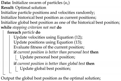 |
Equations for the velocity and the position updates:
where w is the inertia weight, and are acceleration constants typically set to , and are random values in the range [0, 1], represents the historical best position of particle , and is the global best position among all particles.
For step 3
Directly update the Lagrange multiplier .
4. Numerical Experiments
4.1. Numerical Simulation
In this part, we study the effectiveness of the reconstruction algorithm for two examples where the volatility and the fractional order are known. In our numerical experiments, we utilized the parameters mentioned in [32] for consistency; let , the initial value , and other parameters
Example 1.
Considering volatility function , , the Lagrangian multiplier and the update step size of are respectively taken as .
We will use the European put option price calculated using the exact volatility and parameter as the market price of the option. Stop iterating when , where represents the volatility generated by the d-th iteration, and the total number of iterations is not greater than 100. Figure 1 presents a graph of exact volatility versus reconstructed volatility, and the recover value of parameter is 0.7. We add noise with intensity of 0.01, 0.03, and 0.05 to the exact volatility to verify the stability
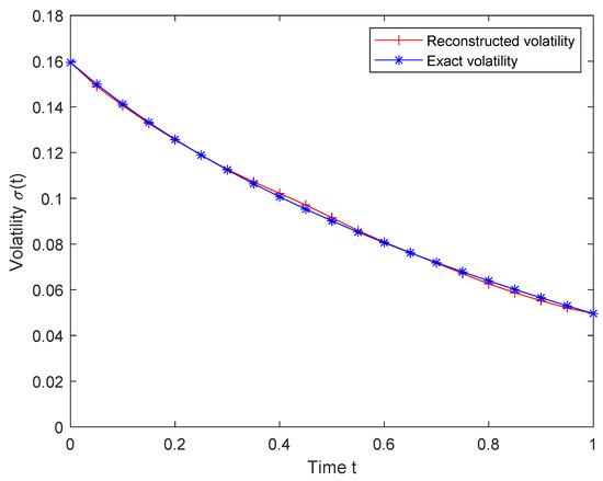
Figure 1.
Exact volatility and reconstructed volatility for Example 1.
We first use perturbed volatility to calculate option prices and then use the resulting option prices to reconstruct fractional and volatility . Figure 2 shows the comparison of real volatility and reconstructed volatility under different noise intensities. Table 1 gives the root mean square error (RMSE), the maximum volatility error, the reconstructed fractional , and the maximum option price error, where RMSE can be calculated by
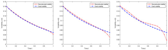
Figure 2.
Real volatility and reconstructed volatility under different noise intensities (left: = 0.01, middle: = 0.03, right: = 0.05) for Example 1.

Table 1.
Numerical results under different intensity disturbances.
Example 2.
In this example, we examine the volatility function represented as , ; the Lagrangian multiplier and the update step size of are respectively taken as
the volatility curve exhibits a smile-shaped pattern.
Figure 3 shows an image of exact volatility versus reconstructed volatility. We can obtain the precise volatility and reconstructed volatility under different noise intensities from Figure 4. Finally, Table 2 shows the RMSE, the absolute error of volatility, and the reconstructed fractional under different noise intensities.
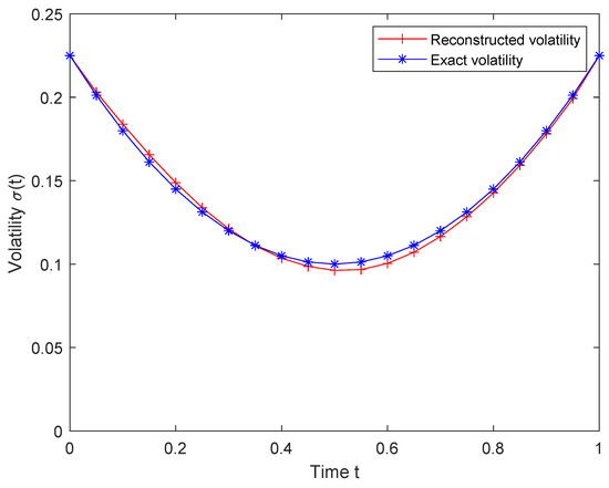
Figure 3.
Exact volatility and reconstructed volatility for Example 2.
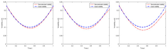
Figure 4.
Real volatility and reconstructed volatility under different noise intensities (left: = 0.01, middle: = 0.03, right: = 0.05) for Example 2.
Table 2.
Numerical results under different intensity disturbances.
4.2. Empirical Analysis
In this part, we utilize the proposed algorithm to recover the volatility function and fractional order based on the Shanghai Stock Exchange (SSE) 50ETF data on 12 December 2023. Table 3 shows real market price for SSE 50ETF put option price with respect to the maturity and strike. The maturity times are and the strike prices are for i = 1, 2, ..., 10. The current value of the underlying asset is , and the interest rate . The Lagrangian multiplier and the update step size of are respectively chosen as
and other parameters are taken as:
Table 3.
The option price of the SSE 50ETF on 12 December 2023.
Figure 5 and Figure 6 depict the comparison between the actual SSE 50ETF market prices and the reconstructed option prices at various time points, complementing the visual analysis, and Table 4 provides information on multiple parameters obtained from the experimental results, and we can obtain , consistent with the recent trends in the SSE 50ETF.
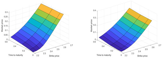
Figure 5.
Left: actual market prices; right: algorithmically reconstructed prices.
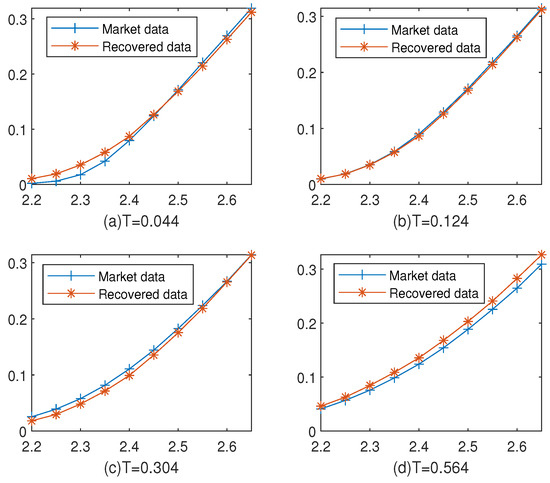
Figure 6.
SSE 50ETF option price and numerical option price at (a) T = 0.044, (b) 0.124, (c) 0.304, and (d) 0.564.
Table 4.
The error outcomes following the calibration of SSE 50ETF options.
5. Conclusions
In this article, we reconstruct both the volatility and the fractional order under the time fractional Vasicke model. Since the calibration problem is ill-posed, we used Tikhonov regularization and the ADMM algorithm for an iterative solution. At the same time, the existence of the solution to the minimization problem is given. And the effectiveness and robustness of the method can be obtained from numerical examples and empirical analysis. From empirical analysis, it can be concluded that is more suitable for the current SSE 50ETF. Furthermore, it serves as an inspiration for readers to employ the derived fractional order in solving time-fractional forward problems, given its relevance to the current Chinese options market. It is worth noting that the possibility of negative interest rates could be addressed by considering alternative models such as the CIR model or CEV model.
Author Contributions
Methodology, project administration, supervision, writing—original, software, draft preparation, Y.D.; data curation, validation, writing—review and editing, Z.X. All authors have read and agreed to the published version of the manuscript.
Funding
This research was funded by the National Natural Science Foundation of China, grant number 12071479.
Data Availability Statement
Data available on request due to restrictions (e.g., privacy, legal or ethical reasons). The data presented in this study are available on request from the corresponding author.
Conflicts of Interest
The authors declare no conflicts of interest.
References
- Black, F.; Scholes, M. The pricing of options and corporate liabilities. J. Political Econ. 1973, 81, 637–654. [Google Scholar] [CrossRef]
- Cox, J.C. The constant elasticity of variance option pricing model. J. Portf. Manag. 1996, 23, 15–17. [Google Scholar] [CrossRef]
- Cox, J.C.; Ingersoll, J.E., Jr.; Ross, S.A. A Theory of the Term Structure of Interest Rates, 2nd ed.; World Scientific: Singapore, 2005. [Google Scholar]
- Vasicek, O. An equilibrium characterization of the term structure. J. Financ. Econ. 1977, 5, 177–188. [Google Scholar] [CrossRef]
- Yao, K.; Liang, Y.S.; Zhang, F. On the connection between the order of the fractional derivative and the Hausdorff dimension of a fractal function. Chaos Soliton Fract. 2009, 41, 2538–2545. [Google Scholar] [CrossRef]
- Sene, N. Fractional model for a class of diffusion-reaction equation represented by the fractional-order derivative. Fractal Fract. 2020, 4, 15. [Google Scholar] [CrossRef]
- Cruz-Duarte, J.M.; Rosales-Garcia, J.; Correa-Cely, C.R.; Garcia-Perez, A.; Avina-Cervantes, J.G. A closed form expression for the Gaussian-based Caputo-Fabrizio fractional derivative for signal processing applications. Commun. Nonlinear Sci. 2018, 61, 138–148. [Google Scholar] [CrossRef]
- Nourian, F.; Lakestani, M.; Sabermahani, S.; Ordokhani, Y. Touchard wavelet technique for solving time-fractional Black-Scholes model. Comput. Appl. Math. 2022, 41, 150. [Google Scholar] [CrossRef]
- Roul, P. Design and analysis of a high order computational technique for time-fractional Black-Scholes model describing option pricing. Math. Method Appl. Sci. 2022, 45, 5592–5611. [Google Scholar] [CrossRef]
- Chen, C.; Wang, Z.; Yang, Y. A new operator splitting method for American options under fractional Black-Scholes models. Comput. Math. Appl. 2019, 77, 2130–2144. [Google Scholar] [CrossRef]
- Cao, J.; Li, C. Finite difference scheme for the time-space fractional diffusion equations. Open Phys. 2013, 11, 1440–1456. [Google Scholar] [CrossRef]
- Li, C.; Chen, A.; Ye, J. Numerical approaches to fractional calculus and fractional ordinary differential equation. J. Comput. Phys. 2011, 230, 3352–3368. [Google Scholar] [CrossRef]
- Gao, G.; Sun, Z.; Zhang, H. A new fractional numerical differentiation formula to approximate the Caputo fractional derivative and its applications. J. Comput. Phys. 2014, 259, 33–50. [Google Scholar] [CrossRef]
- Alikhanov, A.A. A new difference scheme for the time fractional diffusion equation. J. Comput. Phys. 2015, 280, 424–438. [Google Scholar] [CrossRef]
- Cao, J.; Xu, C.; Wang, Z. A High Order Finite Difference/Spectral Approximations to the Time Fractional Diffusion Equations. Adv. Mater. Res. 2014, 875, 781785. [Google Scholar] [CrossRef]
- Cao, J.; Li, C.; Chen, Y.Q. High-order approximation to Caputo derivatives and Caputo-type advection-diffusion equations (II). Adv. Mater. Res. 2015, 18, 735–761. [Google Scholar] [CrossRef]
- Mokhtari, R.; Mostajeran, F. A High Order Formula to Approximate the Caputo Fractional Derivative. Com. Appl. Math. Comput. 2020, 2, 1–29. [Google Scholar] [CrossRef]
- Li, D.; Wu, C.; Zhang, Z. Linearized Galerkin FEMs for nonlinear time fractional parabolic problems with non-smooth solutions in time direction. J. Sci. Comput. 2019, 80, 403–419. [Google Scholar] [CrossRef]
- Zhang, H.; Zeng, F.; Jiang, X.; Karniadakis, G.E. Convergence analysis of the time-stepping numerical methods for time-fractional nonlinear subdiffusion equations. Fract. Calc. Appl. Anal. 2022, 25, 453–487. [Google Scholar] [CrossRef]
- Yuan, W.; Zhang, C.; Li, D. Linearized fast time-stepping schemes for time-space fractional Schrödinger equations. Phys. D 2023, 454, 133865. [Google Scholar] [CrossRef]
- Zhang, H.; Jiang, X. Convergence analysis of a fast second-order time-stepping numerical method for two-dimensional nonlinear time-space fractional Schrödinger equation. Numer. Methods Partial Differ. Equations 2023, 39, 657–677. [Google Scholar] [CrossRef]
- Dupire, B. Pricing with a smile. Risk 1994, 7, 525–546. [Google Scholar]
- Xu, Z.; Jia, X. The calibration of volatility for option pricing models with jump diffusion processes. Appl. Anal. 2019, 98, 810–827. [Google Scholar] [CrossRef]
- Jiang, L.; Chen, Q.; Wang, L.; Zhang, J. A new well-posed algorithm to recover implied local volatility. Quant. Financ. 2003, 3, 451. [Google Scholar] [CrossRef]
- Li, S.; Zhou, Z. Legendre pseudo-spectral method for optimal control problem governed by a time-fractional diffusion equation. Int. J. Comput. Math. 2017, 95, 1308–1325. [Google Scholar] [CrossRef]
- Zhao, J.; Xu, Z. Simultaneous identification of volatility and mean-reverting parameter for European option under fractional CKLS model. Fractal Fract. 2022, 6, 344. [Google Scholar] [CrossRef]
- Yimamu, Y.; Deng, Z. Convergence of Inverse Volatility Problem Based on Degenerate Parabolic Equation. Mathematics 2022, 10, 2608. [Google Scholar] [CrossRef]
- Jiang, L.; Li, C. Mathematical Modeling and Methods of Option Pricing, 1st ed.; World Scientific: Singapore, 2005. [Google Scholar]
- Zhang, H.; Liu, F.; Turner, I.; Yang, Q. Numerical solution of the time fractional black-scholes model governing European options. Comput. Math. Appl. 2016, 71, 1772–1783. [Google Scholar] [CrossRef]
- Tikhonov, A.N. On the solution of ill-posed problems and the method of regularization. Russ. Acad. Sci. 1963, 151, 501–504. [Google Scholar]
- Lagnado, R.; Osher, S. A technique for calibrating derivative security pricing models: Numerical solution of an inverse problem. J. Comput. Financ. 1997, 1, 13–25. [Google Scholar] [CrossRef]
- Kharrat, M.; Arfaoui, H. A new stabled relaxation method for pricing European options under the time-fractional Vasicek model. Comput. Econ. 2023, 61, 1745–1763. [Google Scholar] [CrossRef]
Disclaimer/Publisher’s Note: The statements, opinions and data contained in all publications are solely those of the individual author(s) and contributor(s) and not of MDPI and/or the editor(s). MDPI and/or the editor(s) disclaim responsibility for any injury to people or property resulting from any ideas, methods, instructions or products referred to in the content. |
© 2024 by the authors. Licensee MDPI, Basel, Switzerland. This article is an open access article distributed under the terms and conditions of the Creative Commons Attribution (CC BY) license (https://creativecommons.org/licenses/by/4.0/).