
A Particle Swarm and Smell Agent-Based Hybrid Algorithm for Enhanced Optimization
 ,
,  , , and
Abstract
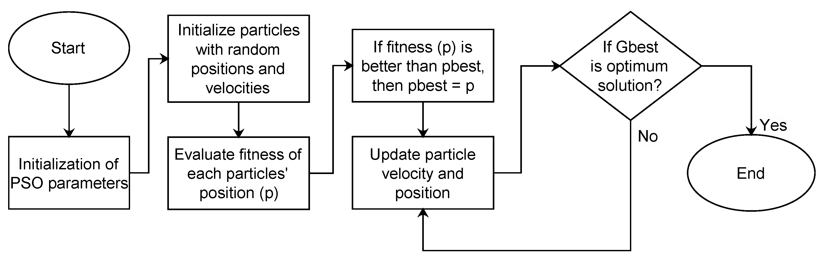
1. Introduction
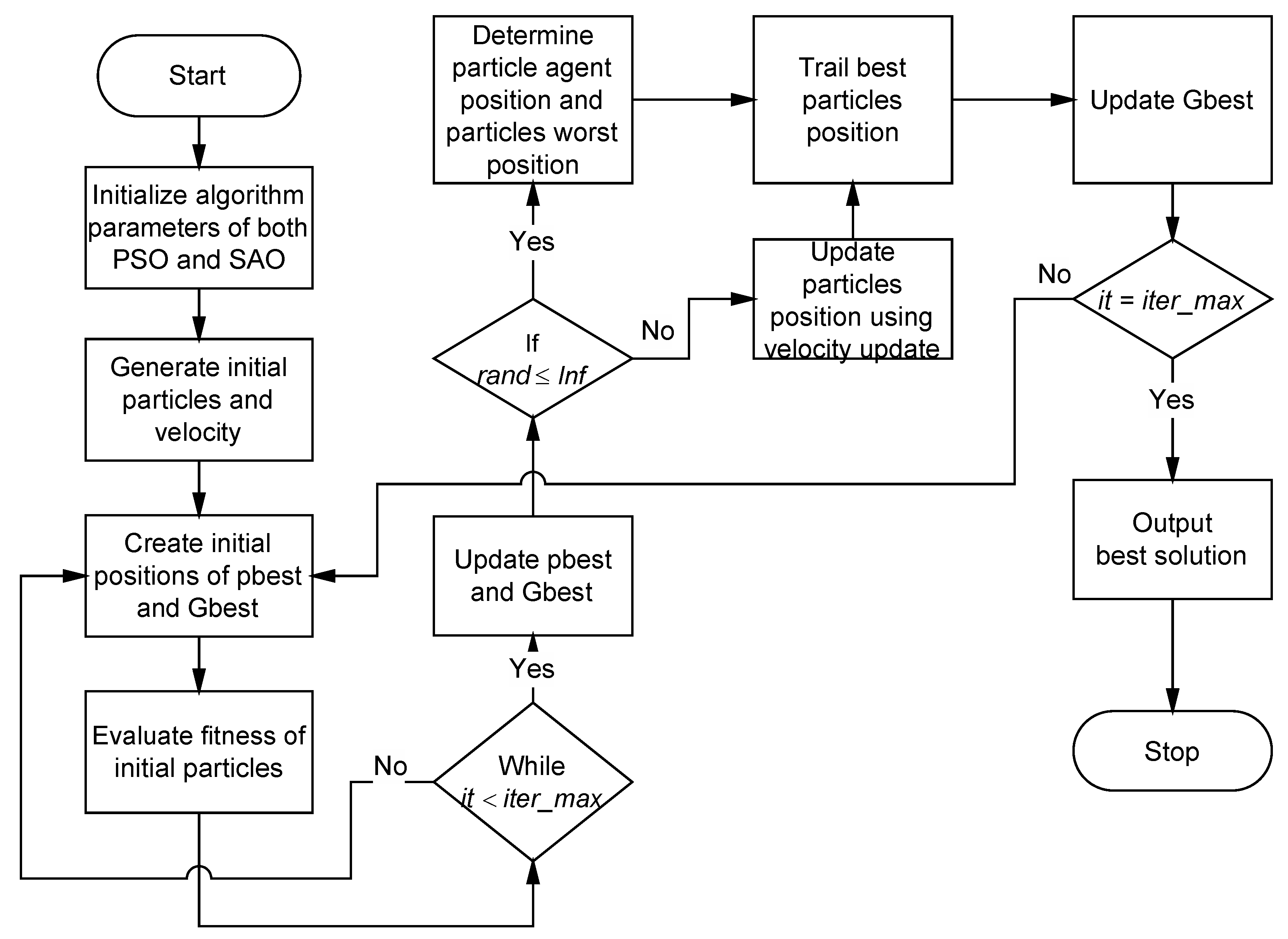
2. Hybridization of PSO and SAO Algorithms
| Algorithm 1: Hopping frequency mechanism deployed in the PSO-SAO for position update |
|
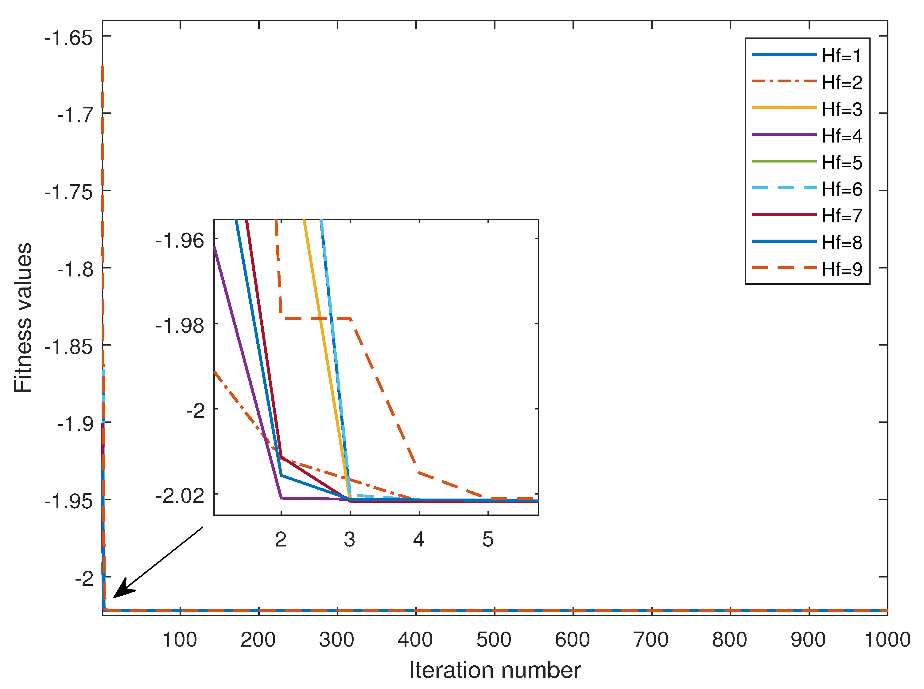
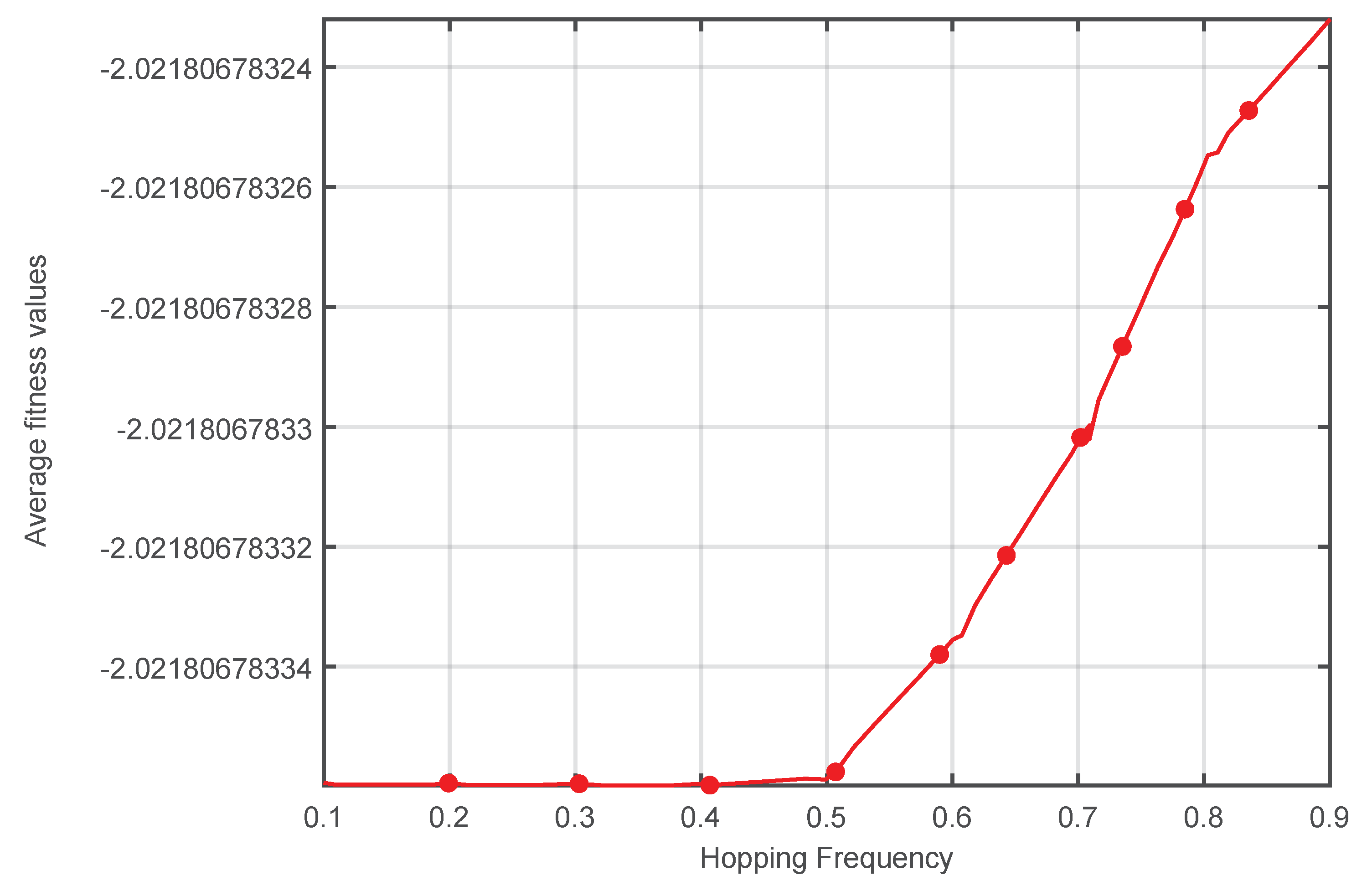
3. Results and Discussion
4. Conclusions
Author Contributions
Funding
Data Availability Statement
Conflicts of Interest
References
- Kennedy, J.; Eberhart, R. Particle swarm optimization. In Proceedings of the ICNN95—International Conference on Neural Networks, Perth, WA, Australia, 27 November–1 December 1995; IEEE: Piscataway, NJ, USA, 1995. ICNN-95. [Google Scholar] [CrossRef]
- Wang, D.; Tan, D.; Liu, L. Particle swarm optimization algorithm: An overview. J. Soft Comput. 2018, 22, 387–408. [Google Scholar] [CrossRef]
- Juneja, M.; Nagar, S. Particle swarm optimization algorithm and its parameters: A review. In Proceedings of the 2016 International Conference on Control, Computing, Communication and Materials (ICCCCM), Allahbad, India, 21–22 October 2016; pp. 1–5. [Google Scholar] [CrossRef]
- Rathod, S.; Saha, A.; Sinha, K. Particle Swarm Optimization and its applications in agricultural research. Food Sci. Rep. 2020, 1, 37–41. [Google Scholar]
- Mythili, K.; Rangaraj, R. Deep Learning with Particle Swarm Based Hyper Parameter Tuning Based Crop Recommendation for Better Crop Yield for Precision Agriculture. Indian J. Sci. Technol. 2021, 14, 1325–1337. [Google Scholar] [CrossRef]
- Raji, I.D.; Bello-Salau, H.; Umoh, I.J.; Onumanyi, A.J.; Adegboye, M.A.; Salawudeen, A.T. Simple deterministic selection-based genetic algorithm for hyperparameter tuning of machine learning models. Appl. Sci. 2022, 12, 1186. [Google Scholar] [CrossRef]
- Bello-Salau, H.; Onumanyi, A.; Sadiq, B.; Ohize, H.; Salawudeen, A.; Aibinu, M. An Adaptive Wavelet Transformation Filtering Algorithm for Improving Road Anomaly Detection and Characterization in Vehicular Technology. Int. J. Electr. Comput. Eng. (IJECE) 2019, 9, 3664–3670. [Google Scholar] [CrossRef]
- Bello-Salau, H.; Aibinu, A.M.; Wang, Z.; Onumanyi, A.J.; Onwuka, E.N.; Dukiya, J.J. An Optimized Routing Algorithm for Vehicle Ad-hoc Networks. Eng. Sci. Technol. Int. J. 2019, 22, 754–766. [Google Scholar] [CrossRef]
- Bello-Salau, H.; Onumanyi, A.J.; Abu-Mahfouz, A.M.; Adejo, A.O.; Mu’Azu, M.B. New Discrete Cuckoo Search Optimization Algorithms for Effective Route Discovery in IoT-Based Vehicular Ad-Hoc Networks. IEEE Access 2020, 8, 145469–145488. [Google Scholar] [CrossRef]
- Valdez, F.; Vazquez, J.C.; Melin, P.; Castillo, O. Comparative Study of the Use of Fuzzy Logic in Improving Particle Swarm Optimization Variants for Mathematical Functions Using Co-evolution. Appl. Soft Comput. 2017, 52, 1070–1083. [Google Scholar] [CrossRef]
- Zheng, R.Z.; Zhang, Y.; Yang, K. A transfer learning-based particle swarm optimization algorithm for the traveling salesman problem. J. Comput. Des. Eng. 2022, 9, 933–948. [Google Scholar]
- Zhong, Y.; Lin, J.; Wang, L.; Zhang, H. Discrete comprehensive learning particle swarm optimization algorithm with Metropolis acceptance criterion for the traveling salesman problem. Swarm Evol. Comput. 2018, 42, 77–88. [Google Scholar] [CrossRef]
- Song, B.; Wang, Z.; Zou, L. An Improved PSO Algorithm for Smooth Path Planning of Mobile Robots Using Continuous High-Degree Bezier Curve. Appl. Soft Comput. 2021, 100, 106960. [Google Scholar] [CrossRef]
- Song, B.; Wang, Z.; Zou, L. On Global Smooth Path Planning for Mobile Robots Using a Novel Multimodal Delayed PSO Algorithm. Cogn. Comput. 2017, 9, 5–17. [Google Scholar] [CrossRef]
- Shami, T.M.; El-Saleh, A.A.; Alswaitti, M.; Al-Tashi, Q.; Summakieh, M.A.; Mirjalili, S. Particle Swarm Optimization: A Comprehensive Survey. IEEE Access 2022, 10, 10031–10061. [Google Scholar] [CrossRef]
- Yang, X.; Jiao, Q.; Liu, X. Center Particle Swarm Optimization Algorithm. In Proceedings of the 2019 IEEE 3rd Information Technology, Networking, Electronic and Automation Control Conference (ITNEC), Chengdu, China, 15–17 March 2019; pp. 2084–2087. [Google Scholar] [CrossRef]
- Bansal, J.C. Particle Swarm Optimization. In Evolutionary and Swarm Intelligence Algorithms; Springer International Publishing: Berlin/Heidelberg, Germany, 2018; pp. 11–23. [Google Scholar] [CrossRef]
- You, Z.; Chen, W.; He, G.; Nan, X. Adaptive Weight Particle Swarm Optimization Algorithm with Constriction Factor. In Proceedings of the 2010 International Conference of Information Science and Management Engineering (ISME), Shaanxi, China, 7–8 August 2010; IEEE: Piscataway, NJ, USA, 2010; Volume 2, pp. 245–248. [Google Scholar] [CrossRef]
- Lu, Y.; Liang, M.; Ye, Z.; Cao, L. Improved Particle Swarm Optimization Algorithm and Its Application in Text Feature Selection. Appl. Soft Comput. 2015, 35, 629–636. [Google Scholar] [CrossRef]
- Wang, F.; Zhang, H.; Li, K.; Lin, Z.; Yang, J.; Shen, X.-L. A Hybrid Particle Swarm Optimization Algorithm Using Adaptive Learning Strategy. Inf. Sci. 2018, 436, 162–177. [Google Scholar] [CrossRef]
- Singh, A.; Sharma, A.; Rajput, S.; Bose, A.; Hu, X. An Investigation on Hybrid Particle Swarm Optimization Algorithms for Parameter Optimization of PV Cells. Electronics 2022, 11, 909. [Google Scholar] [CrossRef]
- Harrison, K.R.; Engelbrecht, A.P.; Ombuki-Berman, B.M.J.S.I. Self-Adaptive Particle Swarm Optimization: A Review and Analysis of Convergence. Swarm Intell. 2018, 12, 187–226. [Google Scholar] [CrossRef]
- Liang, X.; Li, W.; Zhang, Y.; Zhou, M.J.S.C. An Adaptive Particle Swarm Optimization Method Based on Clustering. Soft Comput. 2015, 19, 431–448. [Google Scholar] [CrossRef]
- Zhang, Y.; Gong, D.-W.; Cheng, J. Multi-Objective Particle Swarm Optimization Approach for Cost-Based Feature Selection in Classification. IEEE/ACM Trans. Comput. Biol. Bioinform. 2015, 14, 64–75. [Google Scholar] [CrossRef]
- Cui, Y.; Meng, X.; Qiao, J. A Multi-Objective Particle Swarm Optimization Algorithm Based on Two-Archive Mechanism. Appl. Soft Comput. 2022, 119, 108532. [Google Scholar] [CrossRef]
- Lin, Q.; Li, J.; Du, Z.; Chen, J.; Ming, Z. A Novel Multi-Objective Particle Swarm Optimization With Multiple Search Strategies. Eur. J. Oper. Res. 2015, 247, 732–744. [Google Scholar] [CrossRef]
- Salawudeen, A.T.; Mu’azu, M.B.; Yusuf, A.; Adedokun, E.A. A Novel Smell Agent Optimization (SAO): An Extensive CEC Study and Engineering Application. Knowl. Based Syst. 2021, 232, 107486. [Google Scholar] [CrossRef]
- Mahareek, E.A.; Cifci, M.A.; El-Zohni, H.; Desuky, A.S. Rhizostoma Optimization Algorithm and Its Application in Different Real-World Optimization Problems. Int. J. Electr. Comput. Eng. (IJECE) 2023, 13, 4317–4338. [Google Scholar] [CrossRef]
- Jamil, M.; Yang, X.S. A Literature Survey of Benchmark Functions for Global Optimisation Problems. Int. J. Math. Model. Numer. Optim. 2013, 4, 150–194. [Google Scholar] [CrossRef]
- Salawudeen, A.T.; Mu’azu, M.B.; Yusuf, A.; Adedokun, E.A. From Smell Phenomenon to Smell Agent Optimization (SAO): A Feasibility Study. In Proceedings of the International Conference on Global and Emerging Trends (ICGET 2018), Abuja, Nigeria, 2–4 May 2018. [Google Scholar]


| FNo | Name | D | Formula | C | Range | Fmin |
|---|---|---|---|---|---|---|
| F1 | Adjiman | 2 | NS, MM | [−1, −1; 2, 1] | −2.0218 | |
| F2 | Beale | 2 | NS, UM | [−4.5, 4.5] | 0 | |
| F3 | Bird | 2 | NS, MM | −106.7645 | ||
| F4 | Bohachevsky1 | 2 | NS, MM | [−100, 100] | 0 | |
| F5 | Booth | 2 | NS, UM | [−10, 10] | 0 | |
| F6 | Branin RCOS1 | 2 | NS, MM | [−5, 0; 10, 15] | 0.3979 | |
| F7 | Branin RCOS2 | 2 | NS, MM | [−5; 15] | 5.5590 | |
| F8 | Brent | 2 | NS, UM | [−10; 10] | 0 | |
| F9 | Bukin F6 | 2 | NS, MM | [−15, −3; −3, 3] | 0 | |
| F10 | Camel-Six Hump | 2 | NS, MM | [−5; 5] | −1.0316 | |
| F11 | Chichinadze | 2 | S, MM | [−30; 30] | −43.3159 | |
| F12 | Deckkers-Aarts | 2 | NS, MM | [−20; 20] | −24777 | |
| F13 | Easom | 2 | S, MM | [−100, 100] | −1 | |
| F14 | Matyas | 2 | NS, UM | [−10,10] | 0 | |
| F15 | McComick | 2 | NS, MU | [−10, 10] | −1.9133 | |
| F16 | Michalewicz | 2 | NS, MM | [0, ] | −1.8013 | |
| F17 | Quadratic | 2 | NS, MM | [−10, 10] | −3873.7243 | |
| F18 | Scahffer | 2 | NS, MM | [−100, 100] | 0 | |
| F19 | Styblinski-Tang | 2 | NS, MM | [−5, 5] | −78.332 | |
| F20 | Box-Betts | 3 | NS, MM | [0.9, 1.2; 9, 11.2; 0.9, 1.2] | 0 | |
| F21 | Colville | 4 | NS, MM | [−1,1] | 0 | |
| F22 | Csendes | 4 | S, MM | [−1,1] | 0 | |
| F23 | Michalewicz | 5 | NS, MM | [0, ] | −4.6877 | |
| F24 | Miele Cantrell | 4 | NS, MM | [−1, 1] | 0 | |
| F25 | Step | 5 | S, UM | [−100, 100] | 0 | |
| F26 | Michalewicz | 10 | NS, MM | [0, ] | −9.6602 | |
| F27 | Shubert | 5 | S, MM | [−10, 10] | −186.7309 | |
| F28 | Ackley | 30 | NS, MM | [−32, 32] | 0 | |
| F29 | Brown | 30 | NS, UM | [−1, 4] | 0 | |
| F30 | Ellipsoid | 30 | NS, UM | [−5.12, 5.12] | 0 | |
| F31 | Griewank | 30 | NS, MM | [−100, 100] | 0 | |
| F32 | Mishra | 30 | NS, MM | [0,1] | 2 | |
| F33 | Quartic | 30 | S, MM | [−1.28, 1.28] | 0 | |
| F34 | Rastrigin | 30 | NS, MM | [−5.12, 5.12] | 0 | |
| F35 | Rosenbrock | 30 | NS, UM | [−30, 30] | 0 | |
| F36 | Salomon | 30 | NS, MM | [−100, 100] | 0 | |
| F37 | Sphere | 30 | S, MM | [−100, 100] | 0 |
| S/N | Initialization Parameters | Values |
|---|---|---|
| 1 | Wmax | 0.9 |
| 2 | Wmin | 0.2 |
| 3 | C1 | 2 |
| 4 | C2 | 2 |
| 5 | Olf | 0.75 |
| 6 | hf | 0.3 |
| Function | F1 | F2 | F3 | ||||||
| Metrics | Average | Std | Error | Average | Std | Error | Average | Std | Error |
| SAO | −2.0218 | 9.11 × 10⁻¹⁶ | 0 | 3.81 × 10⁻² | 1.70 × 10⁻¹ | 0.0381 | −106.75 | 6.37 × 100 | 0.0145 |
| PSO | −2.0134 | 6.19 × 10⁻¹ | 0.0084 | 7.62 × 10⁻² | 2.35 × 10⁻¹ | 0.0762 | −105.82 | 4.31 × 100 | 0.9445 |
| PSO-SAO | −2.0218 | 0.00 × 100 | 0 | 1.54 × 10⁻⁷ | 4.73 × 10⁻⁶ | 0.000000154 | −106.78 | 8.63 × 10⁻¹⁵ | 0.0155 |
| Function | F4 | F5 | F6 | ||||||
| Metrics | Average | Std | Error | Average | Std | Error | Average | Std | Error |
| SAO | 0.00 × 100 | 0.00 × 100 | 0 | 4.90 × 10⁻²⁰ | 1.22 × 10⁻¹⁵ | 4.9 × 10⁻²⁰ | 0.3979 | 0.00 × 100 | 0 |
| PSO | 4.59 × 10⁻²⁰ | 4.59 × 10⁻²⁰ | 4.59 × 10⁻²⁰ | 1.52 × 10⁻¹⁵ | 9.00 × 10⁻⁸ | 1.52 × 10⁻¹⁵ | 0.3979 | 0.00 × 100 | 0 |
| PSO-SAO | 0.00 × 100 | 0.00 × 100 | 0 | 0.00 × 100 | 0.00 × 100 | 0 | 0.3979 | 0.00 × 100 | 0 |
| Function | F7 | F8 | F9 | ||||||
| Metrics | Average | Std | Error | Average | Std | Error | Average | Std | Error |
| SAO | −0.2066 | 8.26 × 10⁻² | 5.7656 | 2.88 × 10−78 | 8.58 × 10−78 | 2.88 × 10−78 | 5.10 × 100 | 1.03 × 10⁻¹⁶ | 5.1 |
| PSO | −0.2058 | 6.10 × 10⁻² | 5.7648 | 1.38 × 10−87 | 4.58 × 10−103 | 1.38 × 10−87 | 5.10 × 100 | 1.03 × 10⁻¹⁶ | 5.1 |
| PSO-SAO | −0.2058 | 6.10 × 10⁻² | 5.7648 | 1.38 × 10−87 | 4.58 × 10−103 | 1.38 × 10−87 | 5.10 × 100 | 1.03 × 10⁻¹⁶ | 5.1 |
| Function | F10 | F11 | F12 | ||||||
| Metrics | Average | Std | Error | Average | Std | Error | Average | Std | Error |
| SAO | 5.10 × 100 | 1.03 × 10⁻¹⁶ | 6.1316 | −42.2974 | 42.274 | 1.0185 | −24776.51 | 7.40 × 10⁻¹⁰ | 0.49 |
| PSO | 5.10 × 100 | 1.03 × 10⁻¹⁶ | 6.1316 | −42.2974 | 42.4975 | 1.0185 | −24769.78 | 1.69 × 10⁻⁵ | 7.22 |
| PSO-SAO | 5.10 × 100 | 1.03 × 10⁻¹⁶ | 6.1316 | −42.2974 | 42.4975 | 1.0185 | −24776.51 | 7.40 × 10⁻¹⁰ | 0.49 |
| Function | F13 | F14 | 15 | ||||||
| Metrics | Average | Std | Error | Average | Std | Error | Average | Std | Error |
| SAO | −1.00 × 100 | 0.00 × 100 | 0 | 6.36 × 10−82 | 1.91 × 10−92 | 6.36 × 10−82 | −1.9132 | 4.56 × 10⁻¹⁶ | 1 × 10⁻⁴ |
| PSO | −0.9958 | 3.07 × 10⁻¹ | 0.0042 | 1.67 × 10⁻⁷ | 1.07 × 10⁻⁷ | 0.000000167 | −1.9132 | 4.56 × 10⁻¹⁶ | 1 × 10⁻⁴ |
| PSO-SAO | −1.00 × 100 | 0.00 × 100 | 0 | 3.31 × 10−77 | 1.21 × 10−91 | 3.31 × 10−77 | −1.9132 | 4.56 × 10⁻¹⁶ | 1 × 10⁻⁴ |
| Function | F16 | F17 | F18 | ||||||
| Metrics | Average | Std | Error | Average | Std | Error | Average | Std | Error |
| SAO | −1.9998 | 6.15 × 10⁻¹ | 0.1985 | −3873.72 | 0.00 × 100 | 0.0043 | 1.31 × 10⁻⁹ | 8.11 × 10⁻¹⁰ | 1.31 × 10⁻⁹ |
| PSO | −2 | 0.00 × 100 | 0.1987 | −3497.13 | 1.39 × 100 | 376.5943 | 2.45 × 10⁻¹⁰ | 7.11 × 10⁻¹⁰ | 2.45 × 10⁻¹⁰ |
| PSO-SAO | −2 | 0.00 × 100 | 0.1987 | −3873.72 | 0.00 × 100 | 0.0043 | 2.55 × 10⁻⁷ | 4.10 × 10⁻⁷ | 0.000000255 |
| Function | F19 | F20 | F21 | ||||||
| Metrics | Average | Std | Error | Average | Std | Error | Average | Std | Error |
| SAO | −78.3322 | 1.46 × 10⁻¹⁴ | 0.0002 | 1.26 × 10² | 3.87 × 100 | 126 | 0.00 × 100 | 0.00 × 100 | 0 |
| PSO | −78.3162 | 2.41 × 10⁻¹ | 0.0158 | 1.26 × 10² | 4.37 × 10⁻¹⁴ | 126 | 1.38 × 100 | 1.39 × 100 | 1.38 |
| PSO-SAO | −78.3322 | 1.46 × 10⁻¹⁴ | 0.0002 | 1.26 × 10² | 4.37 × 10⁻¹⁴ | 126 | 0.00 × 100 | 0.00 × 100 | 0 |
| Function | F22 | F23 | F24 | ||||||
| Metrics | Average | Std | Error | Average | Std | Error | Average | Std | Error |
| SAO | 6.71 × 10⁻²⁴ | 0.00 × 100 | 6.71 × 10⁻²⁴ | 4.99 × 10⁻⁹ | 1.43 × 10³ | 4.687700005 | 1.63 × 10⁻⁷ | 1.61 × 10⁻² | 0.000000163 |
| PSO | 3.69 × 10⁻¹⁴ | 4.35 × 10⁻⁹ | 3.69 × 10⁻¹⁴ | −5 | 0.00 × 100 | 0.3123 | 0.00 × 100 | 0.00 × 100 | 0 |
| PSO-SAO | 1.24 × 10⁻²³ | 6.50 × 10⁻⁷ | 1.24 × 10⁻²³ | −5 | 0.00 × 100 | 0.3123 | 0.00 × 100 | 0.00 × 100 | 0 |
| Function | F25 | F26 | F27 | ||||||
| Metrics | Average | Std | Error | Average | Std | Error | Average | Std | Error |
| SAO | 0.00 × 100 | 0.00 × 100 | 0 | −9.9991 | 3.73 × 10⁻³ | 0.3389 | −186.73 | 2.53 × 10⁻¹⁴ | 0.0009 |
| PSO | 0.00 × 100 | 0.00 × 100 | 0 | −10 | 0.00 × 100 | 0.3398 | −170.45 | 5.75 × 10⁻³ | 16.2809 |
| PSO-SAO | 0.00 × 100 | 0.00 × 100 | 0 | −10 | 0.00 × 100 | 0.3398 | −186.73 | 3.91 × 10⁻¹⁴ | 0.0009 |
| Function | F28 | F29 | F30 | ||||||
| Metrics | Average | Std | Error | Average | Std | Error | Average | Std | Error |
| SAO | 8.88 × 10⁻¹⁶ | 0.00 × 100 | 8.88 × 10⁻¹⁶ | 3.00 × 100 | 6.93 × 10−117 | 3 | 9.93 × 10−155 | 3.69 × 10−144 | 9.93 × 10−155 |
| PSO | 8.88 × 10⁻¹⁶ | 0.00 × 100 | 8.88 × 10⁻¹⁶ | 1.41 × 10⁻¹⁵ | 1.48 × 10⁻⁵ | 1.41 × 10⁻¹⁵ | 7.17 × 10−56 | 2.21 × 10⁻¹² | 7.17 × 10−56 |
| PSO-SAO | 8.88 × 10⁻¹⁶ | 0.00 × 100 | 8.88 × 10⁻¹⁶ | 7.00 × 100 | 1.46 × 10−128 | 7 | 1.09 × 10−158 | 4.10 × 10−158 | 1.09 × 10−158 |
| Function | F31 | F32 | F33 | ||||||
| Metrics | Average | Std | Error | Average | Std | Error | Average | Std | Error |
| SAO | 1.02 × 10−38 | 4.48 × 10⁻²² | 1.02 × 10−38 | 2.38 × 10−294 | 0.00 × 100 | 2 | 1.57 × 10⁻⁴ | 0.00 × 100 | 0.000157 |
| PSO | 0.00 × 100 | 0.00 × 100 | 0 | 6.82 × 10² | 2.45 × 10² | 680 | 1.67 × 10⁻² | 1.40 × 10⁻³ | 0.0167 |
| PSO-SAO | 0.00 × 100 | 0.00 × 100 | 0 | 9.00 × 100 | 3.58 × 10⁻⁷ | 7 | 1.34 × 10⁻³ | 0.00 × 100 | 0.00134 |
| Function | F34 | F35 | F36 | ||||||
| Metrics | Average | Std | Error | Average | Std | Error | Average | Std | Error |
| SAO | 0.00 × 100 | 1.90 × 10⁻¹ | 0 | 2.72 × 10⁻¹⁷ | 5.86 × 10⁻¹⁷ | 2.72 × 10⁻¹⁷ | 1.22 × 10−59 | 4.86 × 10−56 | 1.22 × 10−59 |
| PSO | 1.22 × 10⁻¹ | 8.83 × 10⁻¹ | 0.122 | 1.19 × 100 | 1.32 × 100 | 1.19 | 4.00 × 10⁻¹ | 1.13 × 10⁻¹ | 0.4 |
| PSO-SAO | 0.00 × 100 | 0.00 × 100 | 0 | 6.48 × 10⁻²⁵ | 1.49 × 10⁻²⁴ | 6.48 × 10⁻²⁵ | 1.11 × 10−60 | 9.60 × 10−61 | 1.11 × 10−60 |
| Function | F34 | ||||||||
| Metrics | Average | Std | Error | ||||||
| SAO | 5.00 × 10−152 | 2.71 × 10−133 | 5 × 10−152 | ||||||
| PSO | 5.36 × 101 | 1.35 × 10⁻⁵ | 53.6 | ||||||
| PSO-SAO | 1.27 × 10−162 | 5.35 × 10−152 | 1.27 × 10−162 | ||||||
| Ranking | Algorithms | Count of Best Values | Percentage (%) |
|---|---|---|---|
| 1 | PSO-SAO | 28 | 76 |
| 2 | SAO | 23 | 62 |
| 3 | PSO | 15 | 41 |
Disclaimer/Publisher’s Note: The statements, opinions and data contained in all publications are solely those of the individual author(s) and contributor(s) and not of MDPI and/or the editor(s). MDPI and/or the editor(s) disclaim responsibility for any injury to people or property resulting from any ideas, methods, instructions or products referred to in the content. |
© 2024 by the authors. Licensee MDPI, Basel, Switzerland. This article is an open access article distributed under the terms and conditions of the Creative Commons Attribution (CC BY) license (https://creativecommons.org/licenses/by/4.0/).
Share and Cite
Sulaiman, A.T.; Bello-Salau, H.; Onumanyi, A.J.; Mu’azu, M.B.; Adedokun, E.A.; Salawudeen, A.T.; Adekale, A.D. A Particle Swarm and Smell Agent-Based Hybrid Algorithm for Enhanced Optimization. Algorithms 2024, 17, 53. https://doi.org/10.3390/a17020053
Sulaiman AT, Bello-Salau H, Onumanyi AJ, Mu’azu MB, Adedokun EA, Salawudeen AT, Adekale AD. A Particle Swarm and Smell Agent-Based Hybrid Algorithm for Enhanced Optimization. Algorithms. 2024; 17(2):53. https://doi.org/10.3390/a17020053
Chicago/Turabian StyleSulaiman, Abdullahi T., Habeeb Bello-Salau, Adeiza J. Onumanyi, Muhammed B. Mu’azu, Emmanuel A. Adedokun, Ahmed T. Salawudeen, and Abdulfatai D. Adekale. 2024. "A Particle Swarm and Smell Agent-Based Hybrid Algorithm for Enhanced Optimization" Algorithms 17, no. 2: 53. https://doi.org/10.3390/a17020053
APA StyleSulaiman, A. T., Bello-Salau, H., Onumanyi, A. J., Mu’azu, M. B., Adedokun, E. A., Salawudeen, A. T., & Adekale, A. D. (2024). A Particle Swarm and Smell Agent-Based Hybrid Algorithm for Enhanced Optimization. Algorithms, 17(2), 53. https://doi.org/10.3390/a17020053