1. Introduction
Testing whether a point is enclosed by a polygon is a problem that many programmers in numerous fields, such as in computer graphics, geographic information systems, machine vision, or robotics, among others, have certainly come across more than once, as many authors have been asserting for a long time [
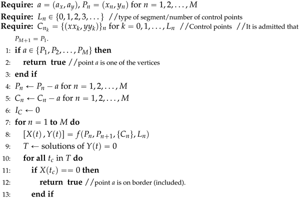
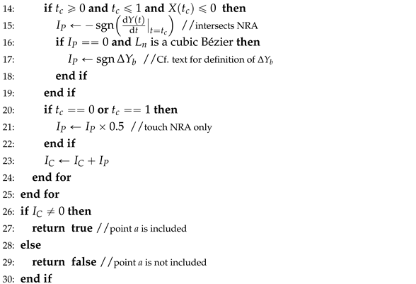
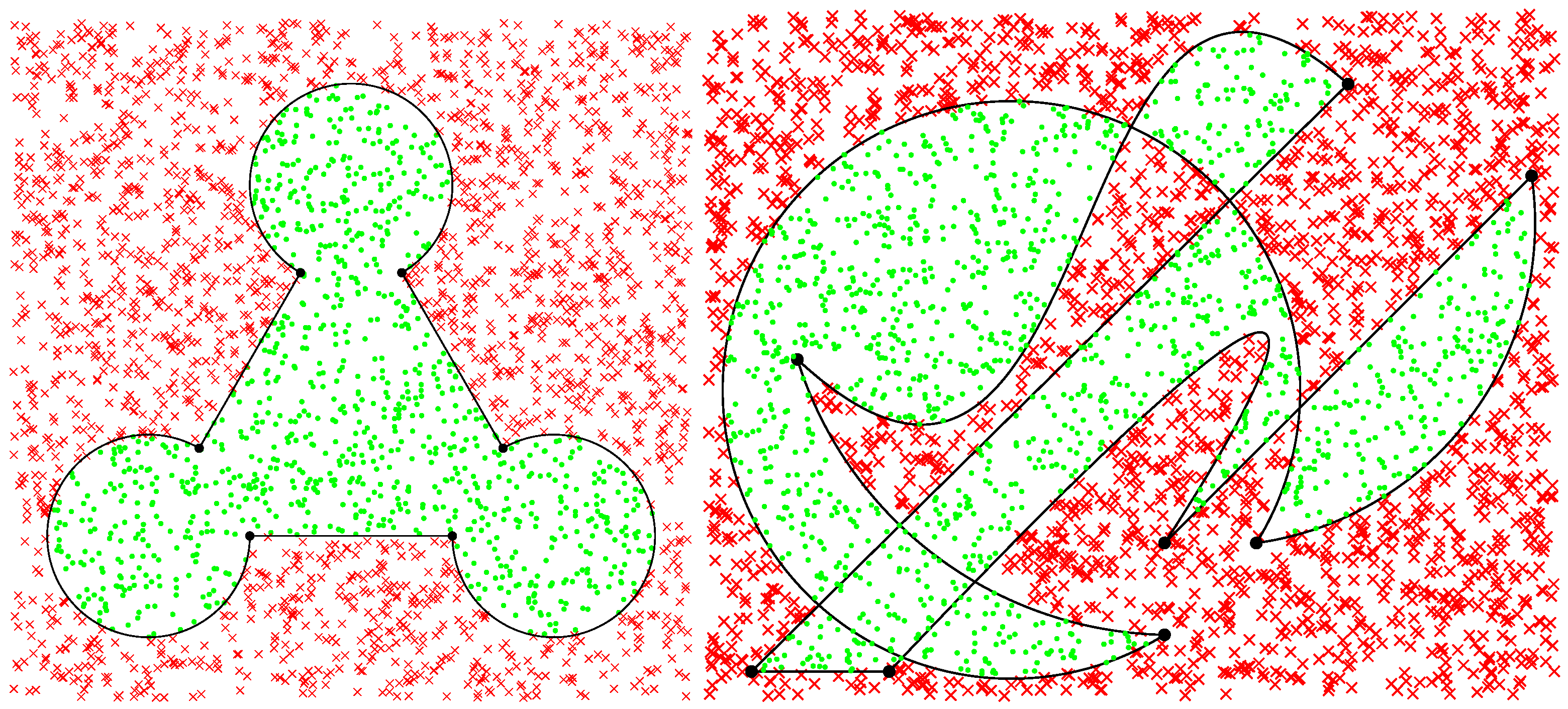
1]. Indeed, the issue is very important and is the object of several concerns in Computational Geometry. It has already been studied and solved for practically all cases of polygonal regions, despite the fact that some earlier algorithms occasionally needed iterative computations, were ambiguous in special cases of on-boundary point locations, or show numerical instability in situations of extreme proximity to borders and vertices. Nonetheless, these limitations are often not very relevant in terms of practical implementation, and the algorithms are actually used on many applications in the software industry. What these algorithms are not aimed at, though, is the analytical evaluation of whether a point lies inside a more complex region bounded by mixed linear and curved segments. Actually, there is no published solution known to the author that indicates how it is possible, with the very same base algorithm and in a straightforward and scalable procedure, to determine analytically, i.e., without linearizing the contour or performing geometric approximations, whether a point is inside or outside regions such as those illustrated in
Figure 1.
2. Related Work
The first known reference to an algorithm for the point location problem dates back to 1962 by M. Shimrat [
2]. That early algorithm had some limitations pointed out soon after by R. Hacker [
3], and later by W. Randolph Franklin, who also states to have delivered, in 1970, a code written in FORTRAN for this same problem [
4]. The books by Preparata and Shamos, published in 1985 [
5], and by Sedgewick, published in 1990 [
6], also covered the point in the polygon problem and have been useful references for many other authors and programmers who have developed specific implementations with adaptations for their own set-ups. Still, nowadays, it is easy to find papers in conferences and journals—in very diverse contexts—where this problem is addressed, even if the novelties have stabilized a long time ago around the two main principles, as described further below.
Eventually, what has become one of the most well-known references in the literature was the publication
Point in Polygon Strategies, in 1994, by Eric Haines [
7], and also some years later, the work of Hormann and Agathos, in 2001 [
8], which is the algorithm being used in Matlab for point location in arbitrary polygons.
A clarification is recommended here to better focus the scope of the paper. Actually, there are two kinds of challenges in this problem: the “point in region” problem, and the “point location in subdivisions of the plane”. Although related, there are some formal differences in these problems.
In the first problem, there is only one region, and we are testing whether a point lies inside or outside of it. In the second problem, there is a group of regions (typically a subdivision of the plane), and we need to identify which specific region the point belongs to. The first problem is to be solved using containment tests specific to the region (e.g., point-in-polygon), and it has constant-time complexity relative to the number of regions but may depend on the complexity of the region’s boundary. The second problem typically involves building a data structure for efficient spatial querying across many regions, with logarithmic or sublinear complexity relative to the number of regions in the subdivision. The second problem usually involves triangulated regions (using Delaunay triangulation), and several works stand out in that front, ranging from the fundamentals from Voronoi diagrams [
9] and Delaunay triangulation, including later optimizations for better data structure management [
10], up to actual point location algorithms in such triangular subdivisions of the plane [
11,
12].
This paper focuses specifically on the first problem and proposes an alternative solution by including additionally the ability to extend the regions to general curve-shaped boundaries. So, in this paper, the expression “point location” refers to assessing whether some point lies inside or outside a given planar region.
2.1. Ray-Crossing Approaches
For a long time, one of the most popular algorithms was the one based on the idea of defining an infinite line starting at the point being analyzed: the number of intersections with the polygon boundary gives indications for the solution, as described, for example, by Preparata and Shamos [
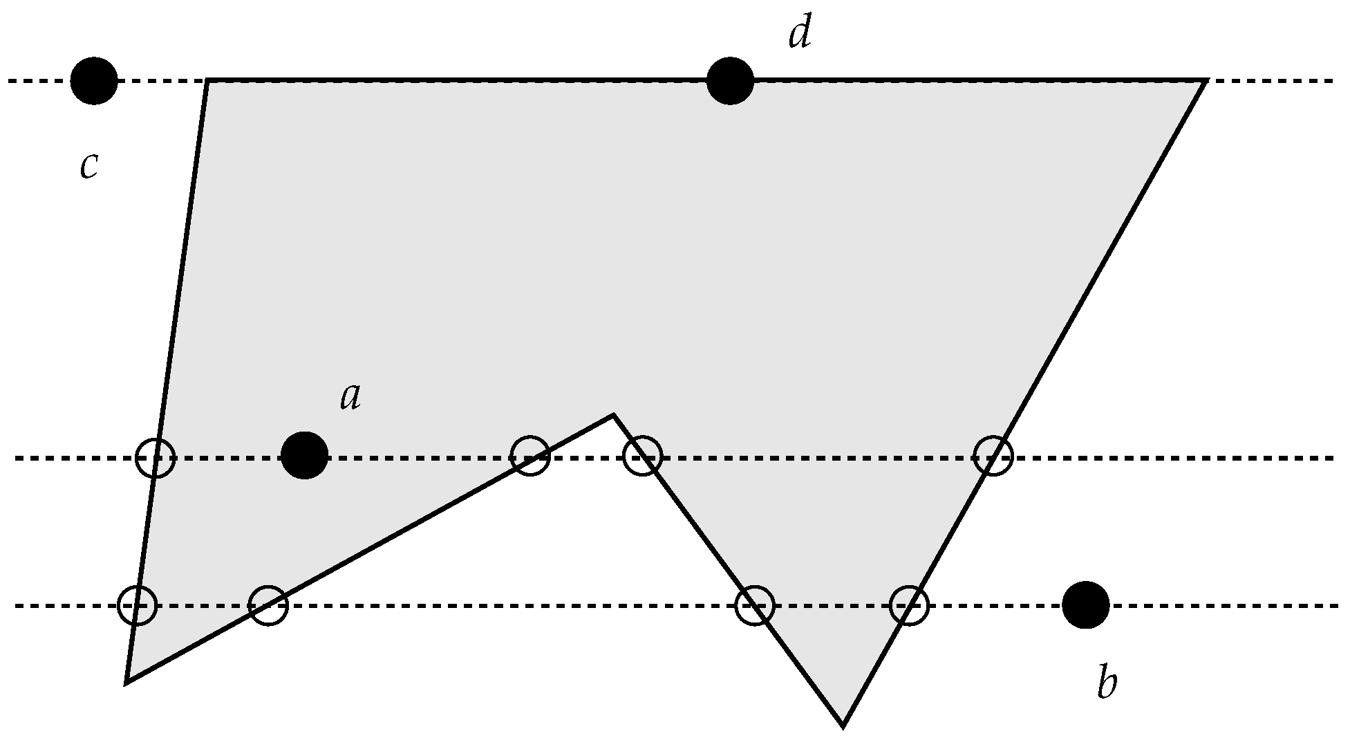
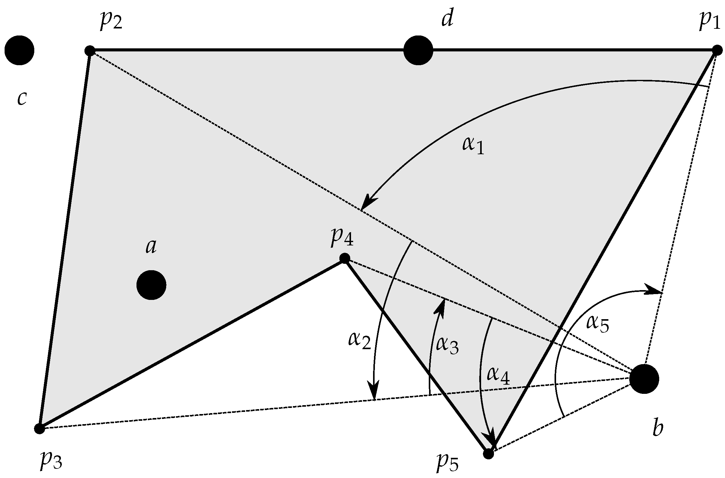
5]. Briefly stated, a point belongs to a polygon if an infinite straight line starting on it intersects the polygon an odd number of times in one direction (
Figure 2). This algorithm is also known as the ray-crossing [
13], the crossing number [
14] algorithm, and the even-odd rule algorithm [
15].
One traditional issue with the ray-crossing algorithm was that it may require further tests to account for the cases where the intersections of the line coincide with one or more vertices or even with an entire edge of the polygon itself. Implementations of this algorithm can be found in many places, and the earlier most well-known implementations occur in the works of Sedgewick [
6], Haines [
7], and O’Rourke [
16].
The ray-crossing algorithm is simple and of limited computational cost,
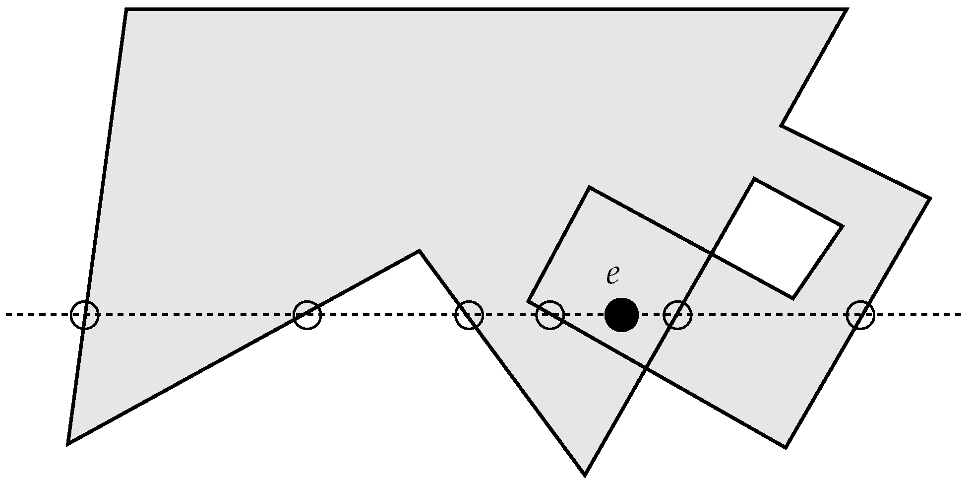
, but, for more functionality, it may require additional steps, hence reducing its elegance. Additionally, applying its technique to generally shaped areas other than polygons, although possible in theory, could pose huge computational and practical difficulties since systems of simultaneous equations might need to be managed and solved. Still, and although it surely has not been intended for that, its applicability for more general self-intersecting (non-simple) domains may fail, as illustrated in
Figure 3, where the point
e would be evaluated as being in the “outside”, which contradicts both the mathematical concept based on the winding number [
17], and the human perception of “insideness” on a folded (and/or twisted) polygon.
2.2. Winding Number Based Approaches
The problem of non-simple polygons (self-intersecting) has nonetheless been practically solved with algorithms based on the winding number [
7], also named nonzero-rule algorithms, which have been refined and even made as efficient as the ray-crossing approach [
14]. Its formulation, based on the sum of all the oriented angles with a center in the test point and delimited by each pair of successive vertices of the polygon, allows to obtain the winding number around a point (the number of times a closed curve winds around a given point in the positive sense), and then conclude whether the point is inside or outside the region. If
are the
M oriented angles defined by the testing point and the
M segments defined with the
M vertices of a polygon, the winding number is calculated by
. If
is equal to zero, then the number of winds of the polygon around the point is zero, meaning that the point is “outside” the polygon. Any other value for
will indicate that the point is “inside” the polygon.
Figure 4 illustrates the geometric principle of the procedure for a simple polygon.
However, the traditional winding number-based algorithms may be ambiguous if the point lies on the boundary and nearly all implementations show some degree of false positives and missed detections, as demonstrated by S. Shirra in [
18]. The technique described generically in
Figure 4 is often seen in the literature as the calculation of the winding number contribution of each linear segment (
) relative to a point
a, where all of the contributions are added up. Mathematically, the procedure is simple, as presented, for example in [
19], and can be easily understood as the calculation of the winding number contribution of that segment relative to the given test point
a:
Demonstration of (1) is straightforward because
and
. In this context
is actually supposed to mean the third component of the actual cross product
. Possible alternative notations would be to replace
in (1) by
, where
, or
or, of course,
.
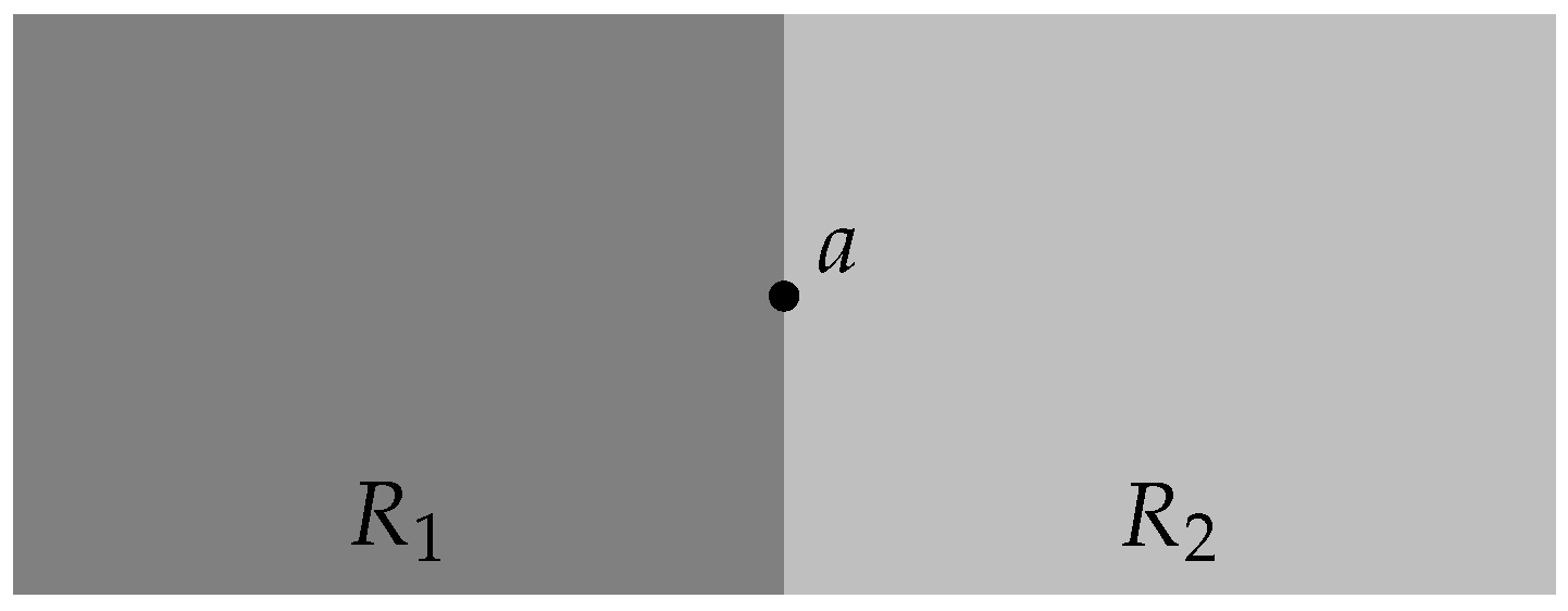
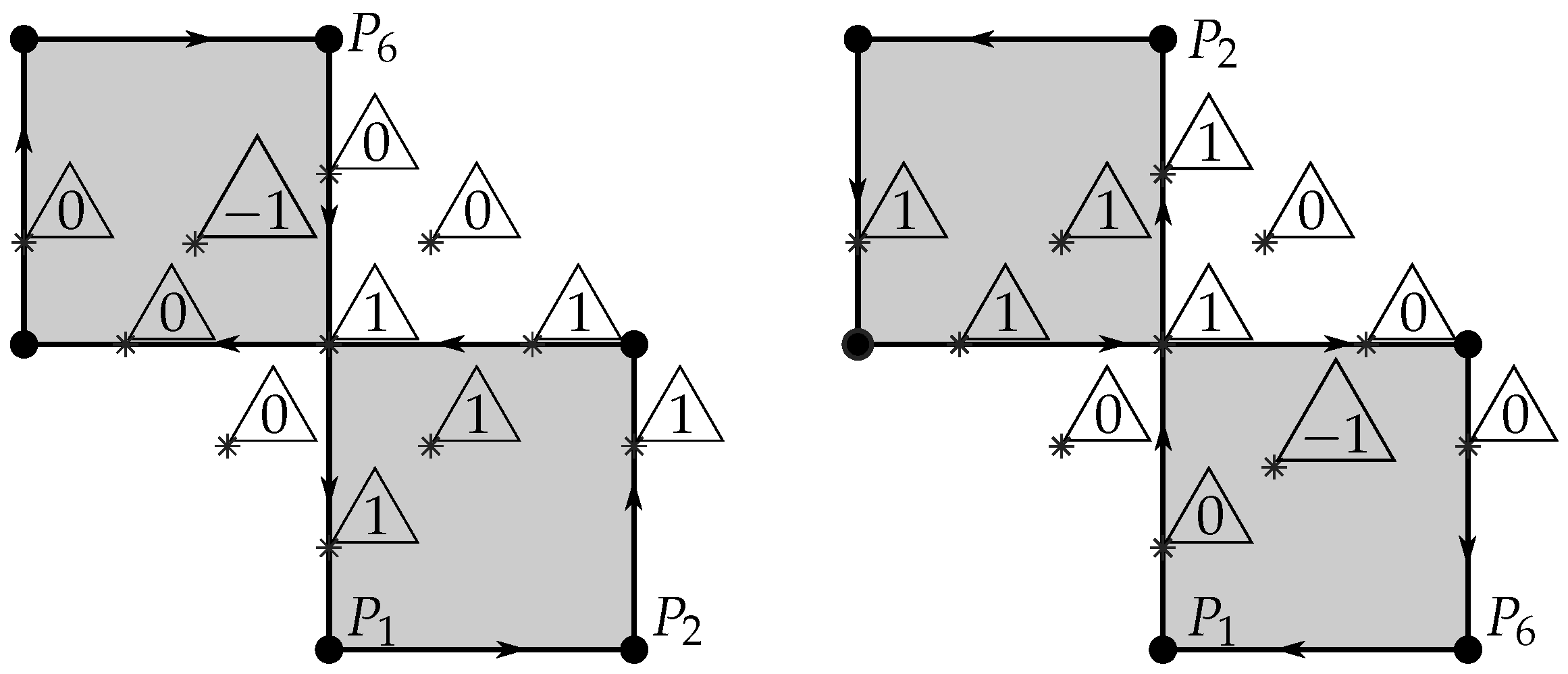
When a point falls over the boundary of a region, more than one interpretation may arise. An example of that occurs in
Figure 5, where two adjacent regions
and
(delimited by different shades and without the border lines being drawn to visually enhance the effect) seem to share a point
a because it falls precisely on the boundaries of the regions. This raises the question of whether point
a belongs to both regions, to only one of them, or neither of them!
The possibility of belonging to neither of the regions must be discarded since a lies in a area covered by both regions altogether, seeming absurd to affirm that a does not belong to neither of the regions and at the same time belonging to their union. So, there remains the possibility of belonging to only or , or both at the same time. This is where the variation of interpretation can take place. If regions are analyzed independently, and using the winding number approach, any conclusion (belonging or not to or ) can be taken depending on the circulation sense of the polygonal lines, as described next. If, on the other hand, the two regions are taken as a degenerate self-intersecting polygon where the common edge is actually a double edge, it will be demonstrated further that a belongs naturally to the compound region (), independently of the circulation sense.
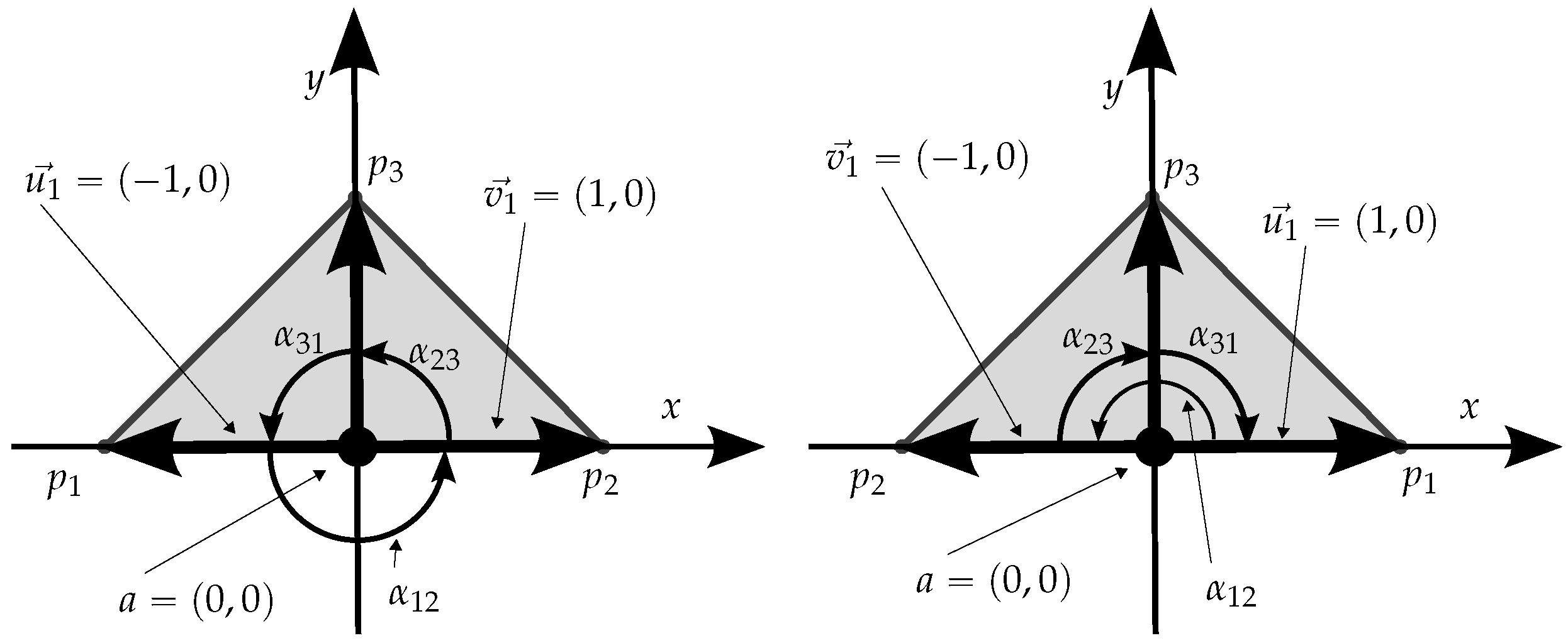
As mentioned earlier, when the testing point is over the boundary, the winding number approach has a variable behavior, depending on the circulation sense, which can be illustrated with this simple example based on a triangle with vertices
,
,
and a test point
. For the triangle longer segment, we have
and
. Also,
and
, and consequently
. If we swap
with
, which is equivalent to reversing the circulation sense, the result is the same for this segment (because it still holds
), which indicates that the approach does not distinguish the sense of circulation (winding number contribution) along a segment when the point is over it. But, for the remainder two segments, the winding number contribution is detected accordingly in different values and, therefore, the overall winding number changes! In conclusion, there are cases where the point will be considered inside and others outside the polygon, depending on the circulation sense.
Figure 6 shows the elements that provide a simple example demonstrating this situation, which is occasionally mentioned by some authors, but also usually dismissed as irrelevant or avoided with specific argumentation, such as in [
4].
Although apparently inconvenient and potentially unexplainable (the sense of circulation was not expected to determine the conclusion of the point inclusion test), this behavior is actually predicted by the Jordan curve theorem.
Indeed, an important concept related to the problem of point location is the well-known Jordan curve theorem (JCT) that, in a simple redaction, as is done in [
20], states that “Every Jordan curve (a non-self-intersecting continuous loop in the plane) separates the plane into exactly two components”. This means that any point is either in one region or in the other, and implicitly, there is no distinct third region, like, for example, “the border”. So, formally, any results derived from the JCT, namely those based on the winding number, may find ambiguity in assessing which of the two regions is the point lying on the boundary, and this is an unavoidable fact that must be managed when using techniques based on circulation or winding number. Actually, for simple curves, when the observer is traveling along the curve counter-clockwise, the points on this curve (boundary), by convention, will belong to the region on the left hand side; so, the identification of which is the “inside” region depends on the traveling (circulation) sense of the observer, and this is where the ambiguity may take place.
2.3. Generalization to Generic Shapes
The generalization of the problem for domains beyond polygons (simple or non-simple) can be carried out by using the winding number approach. However, the literature has not shown a definitive viable implementation to do it, which includes the case of S. Gatilov in [
19], who gives a methodology to calculate the winding angle associated with a circular arc. But Gatilov’s approach counts on the winding number technique described in (1), with its ambiguity for points over segments, which in the case of arcs would be points over the chord of the arc. That is not viable since the point will not even be on the boundary, and the calculation may fail depending on the sense of the circulation! Let us consider the example in
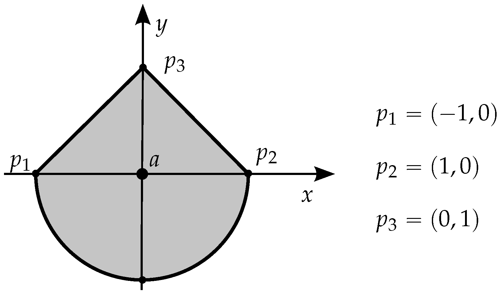
Figure 7 with
. The contribution for the winding number only by the arc
depends on the circulation sense, as happens with any segment, but in case of this arc, the value is not symmetric: it is
or 0! Since the contributions of the other two segments are symmetric depending on the circulation sense (
), this all adds up to ambiguity in detecting whether
a lies inside or outside the region, which is absurd because point
a is clearly inside the region.
Actually, the problem of point location in regions that may have curve segments was first mentioned, although not actually solved in practice, by Edelsbrunner and Maurer in 1981 [
21], and the general problem is seen by Kirkpatrick in 1983 as a challenge that may require a completely new approach:
[…] While the algorithm [proposed by Kirkpatrick] can be adapted to certain other situations (for example, when all internal regions are star shaped), the general problem of optimal search in subdivisions formed from arbitrary curve segments may require a totally new approach. ([
22])
The winding number approach has been a well-accepted solution for the problem of point location, and the calculation of the winding number of a polygonal curve
around some point
a is easy to calculate by determining the number of intersections of
with the real (horizontal) axis, as first pointed out in [
23] and later implemented into a specific algorithm by [
1]. However, in the literature, nothing specific is added concerning the winding number of other curves for the purpose of point inclusion, although algorithms exist to calculate the winding number contribution of Bézier curves [
24].
2.4. Background and Scope of This Paper
This paper demonstrates and gives implementations of a unified approach that covers the traditional solutions based on ray-crossing or winding numbers, solves the cases where those algorithms may find limitations or ambiguities, and extends and demonstrates a practical, viable solution for generic contours that can be expressed in a parametric form, which is its major novelty.
In the early 1990’s, information was not so easy to obtain or track, and faced with the need, the author proposed, during his Ph.D. Thesis [
25], an approach for the problem of point location in polygons based on the Cauchy and Residue theorems, which is closely related to the winding number approach, although unfamiliar at the time.
The algorithm operates by explicitly evaluating contour integrals in the complex plane of a specially chosen function. The solution, found by accidental simplification (it was not fully demonstrated then), proved to work well with a very simple and elegant mathematical formulation. Only later, when formal full mathematical demonstrations were needed, was the current solution developed, as presented in this paper. Hence, it can be said that the solution came to be after the usage of the Cauchy and Residue theorems, but it later became as it it now in its present state. The next sections describe in detail the foundations of the technique, including algorithmic implementations, followed by illustrative results and conclusions.
Code for this research and demonstrations of the algorithms described in the remainder of this paper are publicly available in a GitHub repository (
https://github.com/vitoruapt/PointInclusion (accessed on 2 October 2024)).
3. Base Approach and Related Theorems
The relative location of a point in a polygon, or actually any other form of closed contour in the plane, can be explored by the results provided by the theorem of Residue and the theorem of Cauchy, which are introduced next.
Theorem 1 (Residue Theorem). If is a closed curve of the plane, and is an analytic function in the domain enclosed by Γ (included), except in a finite number of points inside R, then:being the residues of at the singular points inside R (being ). The residue r of a complex function at a point a, which is a pole of order n of f, is calculated by . A complex function is analytic on a region R if it is complex differentiable at every point in R. A common alternative designation is “holomorphic function”, usually the preferable variant by some mathematicians.
Another important fact is given by the Cauchy theorem (or Cauchy–Goursat theorem, since Edouard Goursat (1858–1936) proved this theorem without imposing the condition that
should be continuous inside
and on the boundary, which was an additional condition left by Cauchy [
26]) that states the following:
Theorem 2 (Cauchy–Goursat Theorem). If is a simply or multiply connected region whose boundary Γ is sectionally smooth, and if is analytic in , then the following result applies: The previous statement is actually the formalization of the common expression, which states that a line integral of any analytic function is independent of the path. So, the advantage here is to use non-analytic functions on the regions of interest. After selecting a function that is non-defined in only one point inside
, and whose residue is non-null on that point, by using the Residue and Cauchy theorems, the following reasoning can be engaged:
or, conversely:
Asserting that
is not analytic inside
means that
has at least one discontinuity inside
. Consequently, and being aware that
a is the unique pole (discontinuity) of
in
, i.e., the unique point where it is not defined, a function such as
allows us to state this final and most valuable conclusion: if the contour integral of
along a given contour
is not null, then its pole lies in the region delimited by that contour, or, in mathematical terms:
It is now necessary to draw some considerations to select an appropriate function and the procedures to apply and take advantage of the previous result. Let a boundary
be decomposed in
M parts
with
. After reminding ourselves that a contour integral is no more than a line integral where the integration path is a closed curve, the following is clear:
Although other possibilities exist, we can adopt for
the one suggested earlier and presented in (8):
The residue of at pole a has the value 1. The option for given in (8) is due to the fact that the integrand function should be simple for concerns of computational cost, and that it must possess a non-null residue, which would otherwise lead to inconclusive results. For example, all functions of the type , with , or the type , with , have a residue of 0 on point a, making them useless for this purpose. On the other hand, there are many other possibilities, all with residue 1 at point a, such as the following: , or . However, in all these (usable) alternatives, there would always be the need to calculate a complex logarithm for the anti-derivative. Therefore, the simplest and most obvious case found was precisely the function in expression (8), but, indeed, the principle is independent of the function, which is, however, useful only if it has poles and non-null residues.
4. Calculation of the Contour Integral
If
is analytic in any path between
and
, then the fundamental theorem of calculus along curves applies:
Expression (9) states a very well-known and useful technique, where
is the anti-derivative of
; however, it can be directly applied only if
is continuous along the integration path and
is defined over the integration path; this later condition may not be satisfied when the point being tested is over the contour. Nonetheless, and based on the definition of the Cauchy Principal Value (CPV), the contour integral can still be calculated even if the function being integrated has a pole on the contour. That can be performed by using expression (10) assuming that the pole is enclosed by a circle of radius
, and the fraction of the path outside that circle is named
, where the function
is always integrable independently of how small
becomes [
27]:
Having solved the possible problem of the non-definition of in a finite number of points, it only remains the issue of the continuity of , which is going to be managed with a methodology derived further.
4.1. The Complex Logarithm
The anti-derivative of the chosen function (8) is the logarithm of a complex number, which, formally, is a multi-valued result. By definition, the logarithm of a complex number
z is the number
w that satisfies the expression
. After this definition, it is then clear that the logarithm of
z,
, is multi-valued; if
, using
, and being true that
, the following arises:
It must be noted that the logarithm of a complex number is here graphed with a capital letter to stress its multi-valued nature. With multi-valued expressions, it is not possible to establish comparisons or other relational operations without precautions. The meaning of
depends on the branch where the logarithm is being evaluated, that is, the value of
k in (11). However, the logarithm can be restricted to a single branch, called the principal value, where the imaginary part is unique, hence with only one possible argument, called the principal argument (often designated by the mathematical
function). The principal value is obtained by making
in (11) resulting in:
When restricted to the principal values, logarithms exhibit some particularities like, for example,
equals
rather than
, and, as well,
and not
! As expected, the restriction of the function output to an interval will certainly cause discontinuity of that function and, indeed,
is not continuous for all points of the non-positive real axis because it is clear that:
These issues of the principal value and continuity also affect the logarithms of products (or quotients) when expanded to sums (or subtractions) of logarithms; subtraction or addition of complex logarithms may not always give a result with the imaginary part restricted to the principal value and that is why the following definitions are stated for the logarithm of a quotient, or equivalently, subtraction of logarithms:
and, conversely,
4.2. Line Integral for Linear Segments
Resuming back to the genesis of the algorithm, the essence of the entire procedure is then to evaluate explicitly
and verify whether its value is null or not. It will not be null if
a lies within or over the contour
. By applying (9) to a segment of a path between points
and
, the following result would potentially occur:
4.2.1. Concerns When Calculating the Line Integral
Despite the elegant solution given by (16), there remains the uncertainty of its applicability due to the possible non-continuity of
along the path
. That non-continuity will occur precisely when the path from
to
crosses the negative real axis (NRA), that is, in a neighborhood where
z on the path passes from the 2
nd quadrant (
) to the 3
rd quadrant (
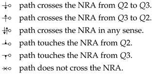
) or vice-versa. The following notation is adopted to define the situations of a path crossing the NRA:
So, the problem is then to calculate the line integral in such conditions of discontinuity, which is explained next. The discontinuity of
occurs when
z crosses the negative real axis, but this effect may occur with other functions apart from the logarithm. So, let us assume that some generic function
f can be parametrized on
(to ease the practical calculation, knowing that
), and its definite integral is to be evaluated from
to
, where
and
are positive angles smaller than
radians, i.e.,
. Being
an infinitesimal positive value, then the following can be written:
From the three terms on the right side of (18), the first and the last are always defined for any value of
(for the functions involved in this analysis). So, taking the limit when
will also force the middle term to be zero because the following holds true for any function
:
Therefore, and being
the anti-derivative of
, expression (18) can be developed into (20):
Expression (20) shows that, when the integration path crosses the negative horizontal axis, the line integral of a function
f, has an additional term of
, whose concrete value depends obviously on the continuity of
. If
happens to be continuous on the value
, then that additional term is null, and we fall back to the fundamental theorem (9). Resuming to the case in discussion, using
=
, then, by taking into account (13), the following holds:
which, by recovering the original variable (
), yields:
A similar reasoning is easy to replicate for the case where the sense of the path is reversed, e.g., swap the integral limits in (20), that is, when the crossing occurs from 3rd quadrant (
) to 2nd quadrant (
), and the result for that case is:
In summary, it can be concluded that the line integral for a path between two points
and
of
is given by:
Considering points
and
to be such that
makes it simple to assert that, for this case, we have:
and consequently, the following always holds true:
Similarly, if we have the reverse situation,
then, the following can also be demonstrated:
In summary, when NRA intersection occurs from
to
(
![Algorithms 17 00444 i023 Algorithms 17 00444 i023]()
), we have the first case in (24) which, by using the equality of case 3 from (15), certified by (27), allows to state the following:
Similarly, when NRA intersection occurs from
to
(
![Algorithms 17 00444 i024 Algorithms 17 00444 i024]()
), we have the second case in (24), which allows us to state the following by using the equality of case 2 from (15), as confirmed by (29):
In conclusion, and by comparing expressions (24) and (15), the following final result is obtained for any
:
A non-null value for expression (32) as the indicator of point inclusion in polygons is precisely the methodology firstly used by the author in [
25] (pp. 149–152), in the early 1990’s, as mentioned before, and whose validity has just been formally demonstrated.
4.2.2. Simplifying the Calculation of the Contour Integral
The result expressed by (32) allows to assert the full methodology because it calculates, directly and in a straightforward mode, the circulation of a path made up of linear segments. In the particular case of
defined as
M linear segments, and with
, expression (7) with the results of expression (32) yields the following generic result:
Furthermore, to simplify the calculation and avoid using at all the complex logarithms, the previous calculations can be even more simplified since the possible variations of the contour calculations only occur in the imaginary part, as it is intuitive from previous statements, and easily demonstrable by expression (34). Indeed, being
and
and therefore
, the calculation of the real part of (33) for the polygon with
M vertices is always null, as shown next:
Finally, it may then be stated that the circulation can be obtained by simply calculating
operations using (35):
Reminding the definition in (14), and being
and
, the definition of the
function for a quotient of two complex numbers is, of course, given by (36):
Resorting to the actual geometric problem, and denoting the testing point by
, and a generic point to delimit segments by
, it is immediate to state that
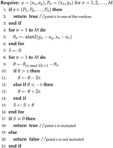
and, hence, Algorithm 1 on the following page can be promptly established. Moreover, since the circulation of
always has a null real part (34), only the imaginary part is relevant and, therefore, the variant for the calculation given by (35) is preferred (simpler) than the calculation using expression (33).
| Algorithm 1: Polygon inclusion test using real |
![Algorithms 17 00444 i005 Algorithms 17 00444 i005]() |
In conclusion, in a closed contour, the neat value of (35) will be null if, along the path, there are no transitions between quadrants and , but if they occur, additional terms of must be added at each time, as expressed by (36). So, the following proposition can be asserted:
Theorem 3 (NRA intersection theorem). In a region enclosing a singularity of a function , the value of the contour integral (hence, the point inclusion) depends exclusively on the number and sense of path transitions over the negative real axis (NRA).
This section has demonstrated how the contour integral is indeed the translation of the winding number approach introduced earlier as one of the well-known techniques for point location in polygons. Moreover, as stated in the NRA intersection theorem, it is also clear that the issues of the winding number calculation (angle contributions) occur only when the path crosses the NRA, which resembles very much the ray crossing method.
4.2.3. Points on the Boundary of Polygons with Undefined Orientation
Algorithm 1 is valid for all combinations of point a and polygon , and requires no post-processing; however, there can be ambiguity in a special situation described next, which is nevertheless easily solvable with a more general approach.
The special situation just mentioned concerns the points over the boundary when the orientation of the polygon (coarsely, the order in which the vertices are browsed) is not the direct orientation, which may give ambiguous results, as expected by the Jordan curve theorem, and mentioned at the beginning of this paper. Indeed, the contour integral
, when
a is over the path
, can result either in 0 or
or, equivalently, a winding number of 0 or 1. Additionally, if the polygon is not simple (i.e., is self-intersecting), the polygon orientation is not adjustable (by reversing the order of vertices, for example) because the orientation changes locally after each self-intersection of the boundary line! For those cases, the contour integral is nonetheless always defined, and
Figure 8 shows several examples of points near a self-intersecting polygon.
In
Figure 8, several observations immediately arise: the first is that clear “outside” and “inside” points are always well determined (winding number of zero or non-zero, respectively). A second observation is that points on the boundary may yield a winding number of 0 or 1, depending on the circulation sense.
There is also a particular case of a point being twice on the boundary (in the intersections), which is always considered “inside”, no matter the sense of circulation. The mentioned ambiguity is however not unsolvable since it is detectable: simply, in case of doubt about the sense of the polygon orientation, to cover even for points over the boundary, a double calculation can be performed: one with the given vertex point order, and the other with its reverse sense; in case one of the calculations yields zero and the other non-zero, then it is the case of a point over the boundary, and further decision can be taken (normally to be considered included in the polygon). This avoids the need of special analysis to detect points on the boundary, which could be absolutely not recommend on general shaped contours, as managed ahead in this paper.
The challenge of points over the boundary is recurrent in all algorithms in the literature. Even one of the most common approaches in the state of the art (the already cited work of Hormann and Agathos [
8] used in Matlab) has a special treatment for the points on the boundary that the authors call
boundary version and is included in Algorithm 7 in their paper, and deals efficiently with points on boundaries of polygons.
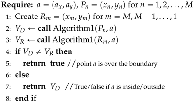
In conclusion, if there can be points anywhere on the boundary that need to be precisely assessed, and there is no knowledge whether a sequence of points of a simple polygon is not given in the positive circulation sense, or whether the polygon is not simple, then Algorithm 1 must be called twice, being the second time done with the polygon vertices in the reverse order. If the two calls of the algorithm yield different results, then we are in the presence of a point over the boundary, and it is (usually) to be considered inside the polygon (Algorithm 2 on the following page).
Algorithm 2 on the next page requires double the computation resources since it calls the actual calculation algorithm twice. This is required only for the absolutely general case of totally random polygons and testing points, although total randomness will hardly generate situations of points exactly over the border. Anyway, alternatives will be presented ahead.
Despite being effective and elegant, in practice, Algorithm 1 is computationally demanding because one trigonometric function (arctan) is used per each side of the polygon, making it less efficient computationally than other alternatives. That, too, is a reason for a change in the paradigm of the calculation, which will align with the existing state of the art algorithms for polygons but also go beyond their performance, not only by outperforming the computational cost but also going where they do not go actually, that is, extension for shapes other than polygons with linear segments. That paradigm is the parametric definition of the integration path.
| Algorithm 2: Unambiguous test for generalized polygons |
![Algorithms 17 00444 i006 Algorithms 17 00444 i006]() |
4.3. Parametric Definition of the Integration Path
An observation that can be made about the technique described in the previous sections is that calculating the line integral for a function with a non-continuous anti-derivative requires care because of the sense of the integration path crossing the NRA, which results in different contributions, as seen. Anyway, for linear segments, the method just described circumvents that issue; however, for non-straight paths to be discussed further, that may not be so clear. Hence, let us adopt an alternative approach to obtain (32) by using parametric integration paths because that explicitly defines a path from a start to an end, along with the variation of the parameter that describes the curve. Let us use a parameter
t that varies from 0 to 1 to cover the full path segment, and let us start with the case of linear segments. Being
and
the extremities of a linear path, any point of the path from
to
is given by:
After adjusting the integration variable,
, the line integral can now be calculated as follows:
that results in:
which is the same as (16), but shares the same risks of discontinuity because the anti-derivative is still a logarithm, despite the fact that the integration variable is now
t. Therefore, the solution is exactly the same as before, given in (22) and (23). In the case of NRA crossing, and depending on the sense (
![Algorithms 17 00444 i010 Algorithms 17 00444 i010]()
or
![Algorithms 17 00444 i011 Algorithms 17 00444 i011]()
), there will be a contribution of
to the contour integral, or
in the NRA crossings counter.
Although it could have been stated and adopted earlier, working for a segment in respect to a point a is actually equivalent to working with segment in respect to . So, from now onwards, when z points are used, it is assumed that they result from the original points subtracted from a, i.e., (), and that the reference point in analysis is the system origin .
5. NRA Crossing in Parametric Paths
We can now settle the procedures to calculate the contour integral along a closed path or, equivalently, the inclusion of a point by a region based solely on the intersection of that path with the NRA.
5.1. NRA Crossings and Their Sense for Linear Segments
What we seek to detect is whether there is an intersection and what is its sense. And this is straightforward to calculate after (38), which can be expanded into:
A NRA intersection occurs at some point
when
and
in
, i.e., intersection occurs for the value
that verifies:
Notice that the case
represents a horizontal segment, and “intersection” only occurs for
. However, that is not actually an intersection of the NRA, as explained later, and this special situation is to be discarded early in the algorithms (also to avoid the division by 0). Apart from that case, if a valid
is found, then it is necessary to determine the sense of the NRA crossing, and that is easily verifiable by the derivative of the imaginary component
in relation to
t. If the derivative is positive for that value of
, it means that the
component is increasing with
t, therefore the path segment is passing from
to
, or
![Algorithms 17 00444 i012 Algorithms 17 00444 i012]()
, that is, there is a contribution of
to the intersection counting (
), or
for the reverse case (
to
, or
![Algorithms 17 00444 i013 Algorithms 17 00444 i013]()
). This can be formalized as:
For linear segments, the previous expression is constant for any point of the segment where the NRA crossing might occur:
If, by chance, the testing point happens to be an intersection point of the polygon boundary with the NRA, either along the path segment ( and ) or strictly on a vertex ( is 0 or 1), that can be promptly detected because its real coordinate would be zero: . This indicates that the point is over the boundary, and a decision can be made immediately without further calculations. Formally: if , then the point is on the boundary, and can be dispatched earlier in the algorithm.
There are also the particular cases of
or
; these represent the cases where the segment starts or ends exactly on the NRA (
![Algorithms 17 00444 i014 Algorithms 17 00444 i014]()
or
![Algorithms 17 00444 i015 Algorithms 17 00444 i015]()
). In those cases, this means that another segment starts or ends there too! To leave the contributions separate, but allowing them to add up or cancel, for those cases, the intersection contribution calculated above should be halved, that is, a
contribution for segments that originate or end on the NRA is to be applied. In other words, each crossing of the NRA can be accounted with
, but reaching or leaving it can be accounted as a half-crossing, or
. Formally, this can be stated as in (45):
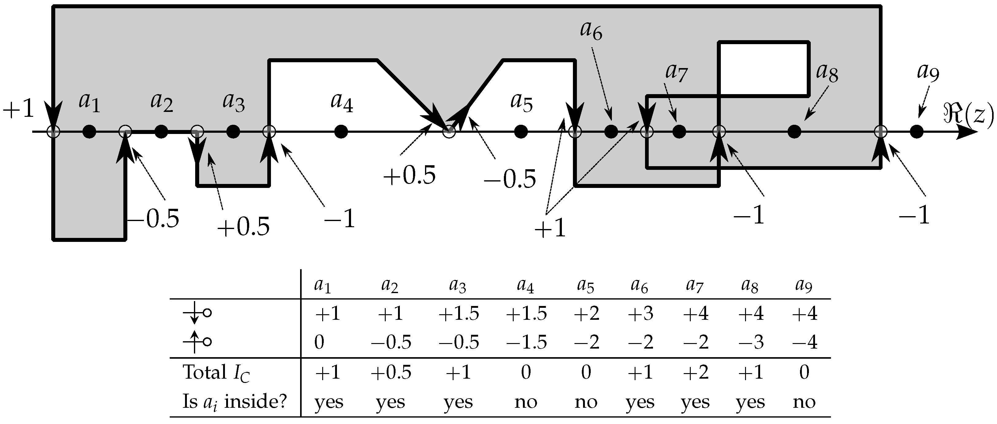
Figure 9 illustrates the situation of
values for several testing points (
) in a polygonal self-intersecting region; the associated table details the partial and total values of NRA intersection counting. At each case (point
), the imaginary axis would be a vertical line that crosses the enclosed domain exactly at each of the
points.
In summary, if a path does not intersect the NRA (
![Algorithms 17 00444 i016 Algorithms 17 00444 i016]()
), the calculation of the line integral is simple (actually, not necessary in practice) because there are no discontinuities in the process and, in the end, all terms of the closed path will cancel altogether; only the intersections of the path with the NRA will affect contour evaluation or the winding number. Also, notice that horizontal segments (
) never intersect NRA; they may even lie over it but never actually cross it, so their contribution to the
is null, as can be seen in the segment that contains the
point in
Figure 9.
The major novelties in this approach for polygonal regions are that the existence of NRA crossing can be determined by detecting the value of a single parameter t and the sense of crossing can be determined by a simple comparison operation.
5.2. The Case of Points on the Border, Again!
In
Figure 9 specific situations arise if the testing point is exactly a NRA crossing point or, which is to say, the testing point is over the border. Once again, this situation forbids the possibility of seamlessly applying a unique algorithm for points on the border. For example, still in
Figure 9, if the testing point occurs on the first crossing point (the one on the left of
), since it has no other crossing on its left, this implies being outside the region; so, its own intersection contribution (
) should be counted to consider it inside. But, if this reasoning is applied to the 4
th intersection (between
and
), then the overall contribution at that point (
) would result in 0 and that point would be considered outside the region, contrarily to the intention of considering it as inside. The conclusion is that there is no unique solution to distinguish with the same operation whether a point on the border is always considered inside or outside the region: this is unavoidable, as supported by the Jordan curve theorem presented earlier, where the sense of crossing (circulation) affects the winding contribution, and therefore the conclusion about inclusion. The solution, as already mentioned, is to check those situations before further calculation.
5.3. Universal Algorithm for Arbitrary Polygons
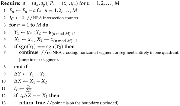
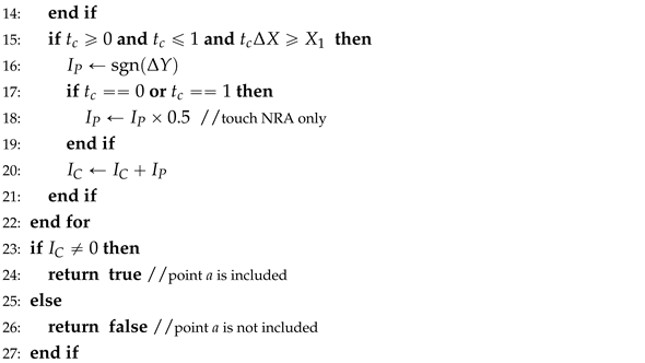
All of the previous procedures are integrated in Algorithm 3, which shows all the steps to test polygonal inclusion of any point
a on any polygon with
M vertices (for any
, but only
is really meaningful), normal or self-intersecting.
| Algorithm 3: Universal inclusion test in arbitrary polygons |
![Algorithms 17 00444 i007a Algorithms 17 00444 i007a]() ![Algorithms 17 00444 i007b Algorithms 17 00444 i007b]() |
The computational cost of Algorithm 3 is , and the arithmetic operations involved are only sums (or subtractions) and at most M floating point divisions per polygon, although optimizable, as described further.
In Algorithm 3, the points on the border, including vertices, are considered inside the polygon, but, if wanted otherwise, this can be easily modified to exclude them. It can be done either with an optional initial checking for a being one of the vertices or during the normal flow of the algorithm after test from line 12 that results from the NRA crossing conditions in expression (42). The decision on line 13 of Algorithm 3 could be set to false if the point on the boundary is defined as being outside.
Notice also that the apparent risk of division by zero in line 11 of the algorithm never occurs because of early analysis in line 6 of the algorithm; indeed, if , we also have and the algorithm skips to the next segment since there is no contribution of the current linear segment to the value of . Illustration of the functionality and results of Algorithm 3 can be found in the GitHub repository indicated earlier.
5.4. Multi-Ring Polygons and Multi-Polygons
There is a category of planar domains commonly used in Geographical Information Systems (GIS), namely to represent contours of countries and other geographical entities, that accounts both for multiple separate polygons (multi-polygons) or for polygons that include “holes” defined by one (or more) separate closed lines fully included in the outer polygon; each of these separate contours is named a ring. A simple polygon has one ring, and a polygon with two “holes” has three rings [
28]. There are also strict cases of multi-ring multi-polygons where rings nest inside each other. All these situations can be handled with the same concepts described earlier using the sense or circulation of a contour.
Figure 10 illustrates three situations of multi-ring polygons.
The figure also illustrates the need for defining correctly the sequence of the polygon vertices in order to apply the same concepts of winding sense and, therefore, obtain the number of NRA intersections. Extension of the algorithm to this type of region is achieved by simply applying the procedure on each of the 2, 3, or more contours (rings) and sum up the separate results of NRA intersections.
5.5. Optimizing Algorithm 3
Algorithm 3 on the preceding page can be computationally alleviated by avoiding unnecessary divisions in case the NRA intersection does not occur. Indeed, as required by expression (42), for NRA intersection to occur we must have the following:
. In other words, if either
or
, then the NRA intersection does not occur, and no more calculations need to be performed. So, a few comparisons (3 at most) can be made before asserting the need to perform the division to find the actual
of NRA intersection. Since
, consider the following:
which can be combined. We are allowed to state that there is no NRA intersection if the following occurs:
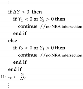
Hence, just before line 11 of Algorithm 3 a few lines could be added to optimize the procedure, demonstrating also that at most 3 comparisons are needed to conclude whether there is NRA intersection or not before calculating
, as proposed next:
![Algorithms 17 00444 i025 Algorithms 17 00444 i025]()
Previous expressions can be further optimized because when they are reached, it is already known that . Therefore, is equivalent to only one of them, e.g., . A similar reasoning applies to the “else”. This further reduces the number of comparisons from 3 to 2.
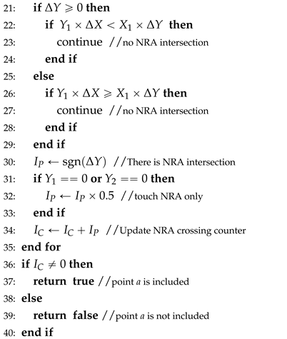
In case there is intersection (i.e., the previous tests concluded that there may be a NRA intersection because ), it is then necessary to calculate its precise value to test the second requirement of expression (42), that is, check the condition , which at first glance seems unavoidable to calculate through the division. But, actually, that division operation can be avoided and replaced by two multiplications and a comparison, as is shown next: being and , if then, for NRA crossing, we need to have: , otherwise, we need to have the following: .
The conclusion is summarized by expression (49):
This last simplification not only avoids the mathematical division butalso allows the algorithm to fully operate in integer arithmetic representation, which would improve its usage in an approach based purely on the integer representation of points/vertices.
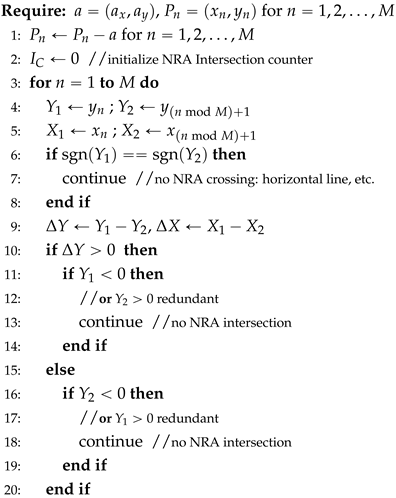
Yet, in line 17, Algorithm 3 still requires to check whether is equal to 0 or to 1 to conclude if the “crossing” is actually a “touching”, which would imply an adjustment on the intersection counter. But that checking turns out redundant because those cases correspond to or , that is, there is no need to calculate for those cases either.
In summary, the algorithm in its full extension and covering all these optimizations, is detailed as Algorithm 4 on the next page. It can be noted, in line 32, that a multiplication by is present, which, although being a statistically rare situation, could be modified for further optimization; that would be to count each full crossing as an integer of value , by, for example, changing line 30 into , and a half crossing being half of that value () with the final conclusions still holding, and integer computations could be present throughout the entire algorithm.
In conclusion, besides the simplicity of the formulation, the algorithm has also the virtue of a straightforward operation with degeneracy situations, such as point over segments or over vertices, or even as null length segments, which could happen in situations of rounding the point representation to integers.
5.6. Vectorization of Algorithm 4
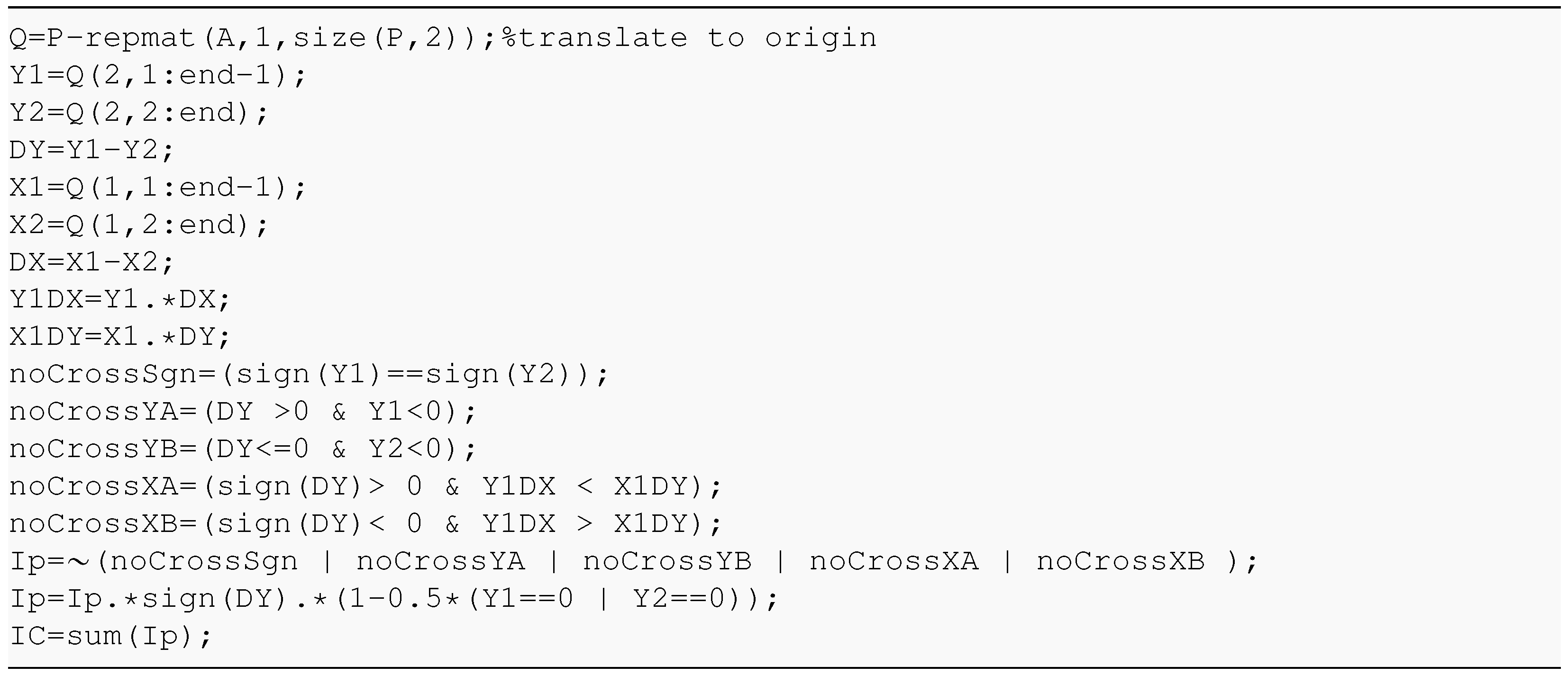
Although not necessarily a breakthrough in reducing computational costs, Algorithm 4 on the following page can be easily vectorized for parallel computing, at least for the test of the inclusion of one point. Follows in
Figure 11 a fully operational excerpt in Matlab code (listing) that accepts a matrix
P with the polygon vertices (with the last vertex replicated from the first) and a point
A. The procedure is vector based and operates with an entire polygon “at once”.
Despite the possibility of some finer tuning, the vectorized approach, nevertheless, forces all the operations to be performed through the entire chain of tests. Some tests could be dismissed early in a sequential approach, but the vector approach forces all the operations for all cases. Hence, it may not be suited for better performance in all computational setups.
| Algorithm 4: An optimized version of Algorithm 3 |
![Algorithms 17 00444 i008a Algorithms 17 00444 i008a]() ![Algorithms 17 00444 i008b Algorithms 17 00444 i008b]() |
5.7. Comparison to the State-of-the-Art Algorithm
For several years, Matlab has been using a version based on the algorithm from Hormann and Agathos [
8], valid for point location in arbitrary polygons. According to the original paper, that algorithm is based on three steps, which, on the optimized variant, includes the following operations:
Evaluation of the determinant: performs 2 multiplications and 1 subtraction per segment;
Quadrant classification: uses 6 comparisons per vertex;
Determination of winding number: performs 2 subtractions/sums and up to 4 + 1 comparisons per vertex.
Algorithm 4 has more steps (though simpler) than Algorithm 3 and requires:
Initial test: 1 sign comparison per vertex;
Coordinate differences: 2 per vertex;
Y coordinate conditions: up to 3 comparisons per vertex;
Test NRA: 2 multiplications and 2 comparisons per vertex;
Test special cases end points: 2 comparisons with zero;
Crossing counter: 1 addition per NRA crossing.
The comparison is given side-by-side in
Table 1, where it can be seen that Algorithm 4 has fewer comparisons (1 + 2 + 2 + 2 = 7 vs. 10 + 1 = 11) and potentially much less if tests dismiss early; there is a similar number of additions/sums: 2 + 1 vs. 3; the multiplications are in equal number but the advantage is that in Algorithm 4 they are needed only when x-axis intersection occurs. In the previous analysis,
subtractions were omitted, reporting to the relocation of the polygon around point
, but which is a common operation to all.
An illustrative example of simple benchmarking is shown in
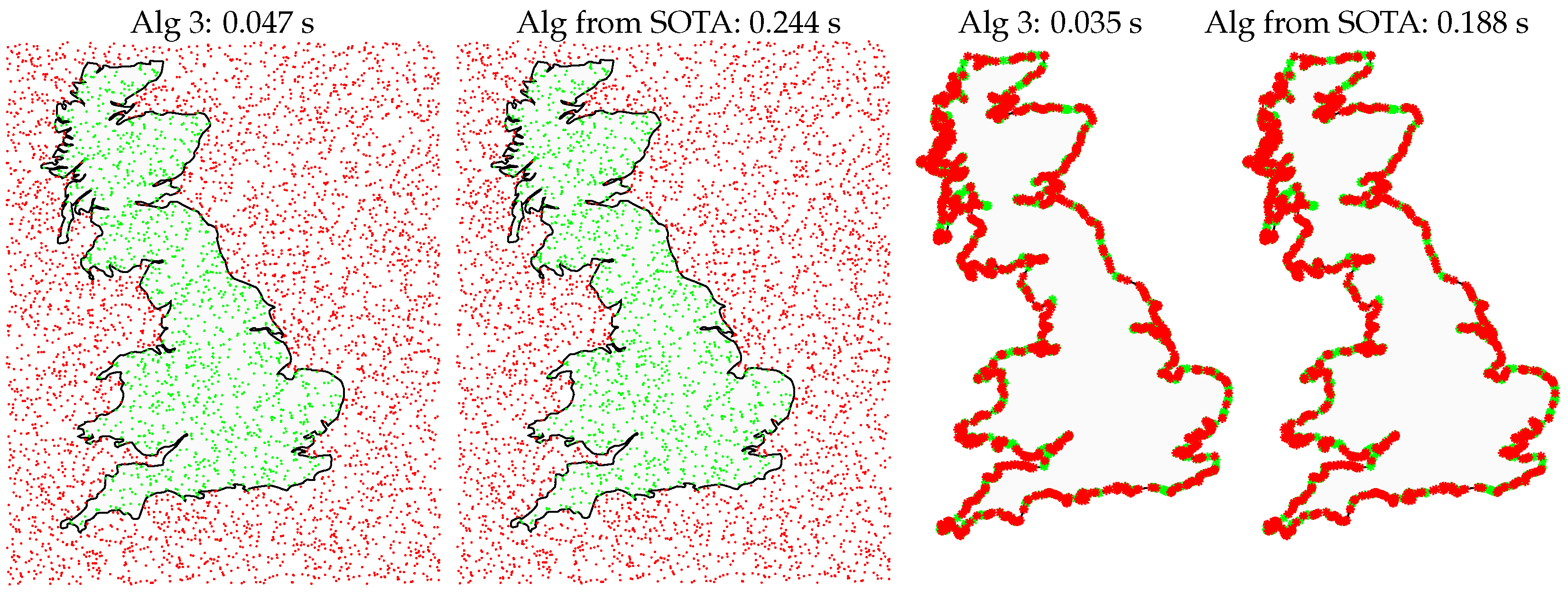
Figure 12 with a polygon with more than 2200 sides and thousands of testing points in two situations: on the left, 5000 completely random points, and on the right more than 2200 points near the border. Results are shown for Algorithm 3 and the state-of-the-art algorithm in Matlab [
8]. The result shown is the average of 100 runs and had the same outcome in both algorithms. In both cases, Algorithm 3 proposed in this paper outperforms by a factor of about 5.
6. NRA Crossing and Sense for Circular Arcs
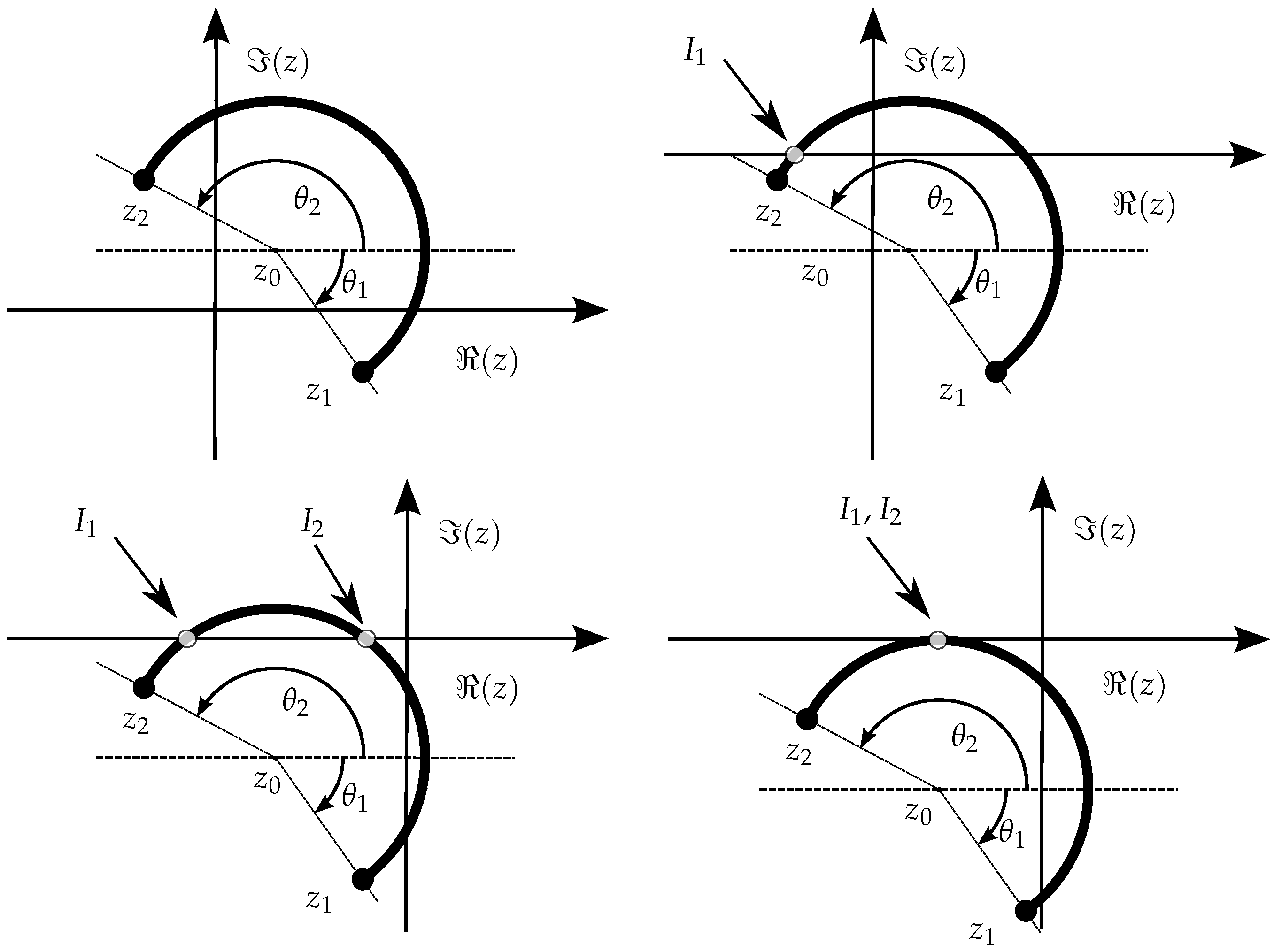
For circular arcs, a few changes occur relative to linear segments. What is the most apparent is the fact that circular arcs can cross the NRA more than once or may even be tangent (
Figure 13). Moreover, the parametric definition of arcs is a little more elaborate than for straight lines, as described next.
6.1. Parametric Expression for Circular Arcs
Any point of a circular arc with center at , and evolving in the positive sense (counter-clockwise—), between point and point is expressed by , where covers the interval defined by and , and .
To simplify the parametrization and unify the procedures used for the linear segment, the following parametric representation is used:
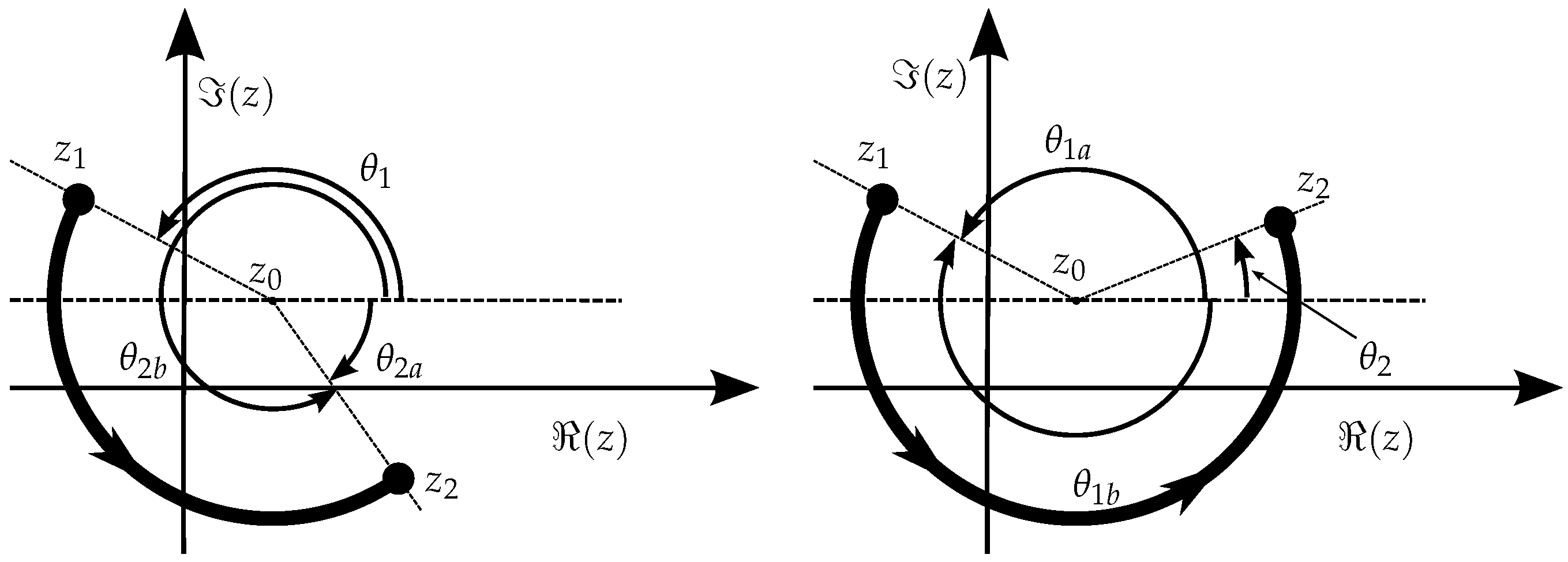
However, to ensure an unambiguous interpretation of the path described for the positive sense, it must be where it is expected that the angles are obtained by the following operations: and . But if that is not the case, then one of the angles must be converted by modulus , that is, force and to fall in the interval , by applying either or , depending on the necessary case.
All the situations in
Figure 13 respect the proper condition,
, but different situations are illustrated in
Figure 14 where
encounters a discontinuity if restricted to the interval
. As the figure explains, in one case the solution for a proper parametrization is to convert
into
and the other to convert
into
.
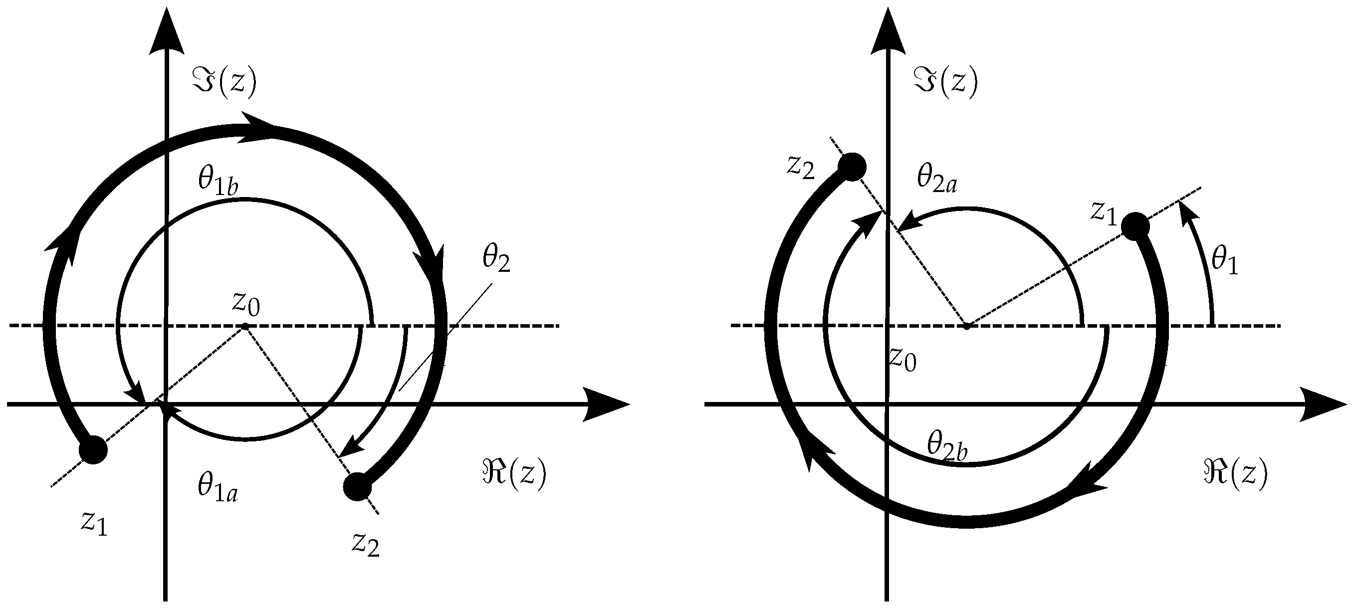
On the other hand, if a negative (or clockwise,
) sense is intended, an equivalent operation must be taken into account, as illustrated in
Figure 15.
In summary, to ensure the proper and unambiguous parametrization of a circular segment, the following steps have to be carried out when defining a circular boundary segment:
Indicate , , and the center (or some other means to obtain , like a third point , or a radius and the relative placement of the center);
Obtain and ;
Define circulation sense ( or );
Check the potential angle adjustments given by (51):
In expression (51), the verification of the equality between and is also considered to include the situation of complete circles (where and would coincide, but actually one of them should be larger than the other to ensure that the possibility of a full circle is covered).
Having the circular path segments duly defined and parametrized, the calculation of the NRA intersections is as straightforward as for the linear segment. Hence, to adapt for the circular arc, there must exist one (or two) values for
t that generate an NRA crossing, and let us call them
:
or in expanded view:
For the same conditions as before,
and
as seen in Section sec:NRAcrossingParametricPaths, we then have:
However, since the circle can cross the NRA twice, two solutions would be expected for
in the second equation of (54); indeed, the total number of solutions in
of an equation of the type
is given by the following:
that, when restricted to the
interval, simplifies into, at most, the following 5 solutions:
Resuming to the variables from (54), we have
where all those potential solutions, besides needing to verify the condition
, must also verify the first condition of (54), that is,
.
Naturally, at most two of the solutions from (57) are valid (two intersections of the x axis), but there can be only one, or even no, solutions at all. As just mentioned, both potential solutions (let us name them and ) must be tested whether they verify expression (54). Nonetheless, there are obvious cases that can be tested beforehand to accelerate the numeric algorithms: one is , resulting in a clear impossibility, and the other case is when , implying that the arc is tangent to the x axis.
For the case of circular arcs, the situation of tangency may be interpreted as either a non-intersection or a double touching of the NRA (entering and leaving the NRA at the same point). The net additional contribution for the calculation of the line integral is, therefore, zero. Hence, if , then the circular segment does not affect the intersection counter . The exception occurs in case the tangency point () happens for being 0 or 1, which is a “half intersection”, as described next.
6.2. Sense of NRA Crossing for Circular Arcs
As before, in case there is an NRA intersection, its sense must be determined, and expression (43) can be used and adapted for the case of arcs:
Expression (58) can be further simplified avoiding the need to calculate the trigonometric function. Knowing that
and being
, we have:
Also, as occurred for the linear segments, the particular cases of or correspond to “half intersections” (one extremity of the arc is over the NRA) and, therefore, the calculated with (59) must be adjusted the same way, as given by (45), or formally stated:
7. Application to Bézier Curves
Most planar domains can be defined by closed splines or other arbitrary curve segments, delimited by two extreme (anchor) points and some control points in a parametric way, which is most frequently of a polynomial nature.Each segment can however be treated the same way as was demonstrated earlier for linear and circular segments. For example, Bézier curves of order
n in the complex plane can be defined by:
where
are the control points, starting at
and ending at
(the anchor points), and with
.
Segments are described by polynomials, making it easy both to differentiate and find roots, except for higher orders (like 5, 6, or more), and in that case, it can represent a challenge for analytical approaches, although numerical approaches are always possible. Bézier curves can also be expressed in the more compact notation:
from which follows an example of a Bézier segment of the 3
rd order, which is one of the most commonly used, thus, representative of many challenges in computational geometry:
or, in full expansion:
As described earlier, detecting the NRA crossing of such a segment requires the solution of
, which would yield up to 3 results for
t in the
interval. If less than 3 NRA intersections occur, this means that some solutions for
t are complex, and are to be discarded. To determine the sense of growing at the intersection points with the NRA, the derivative of
in order to
t is required, and that too is a direct operation easily allowed by the polynomial representation of the curve segment:
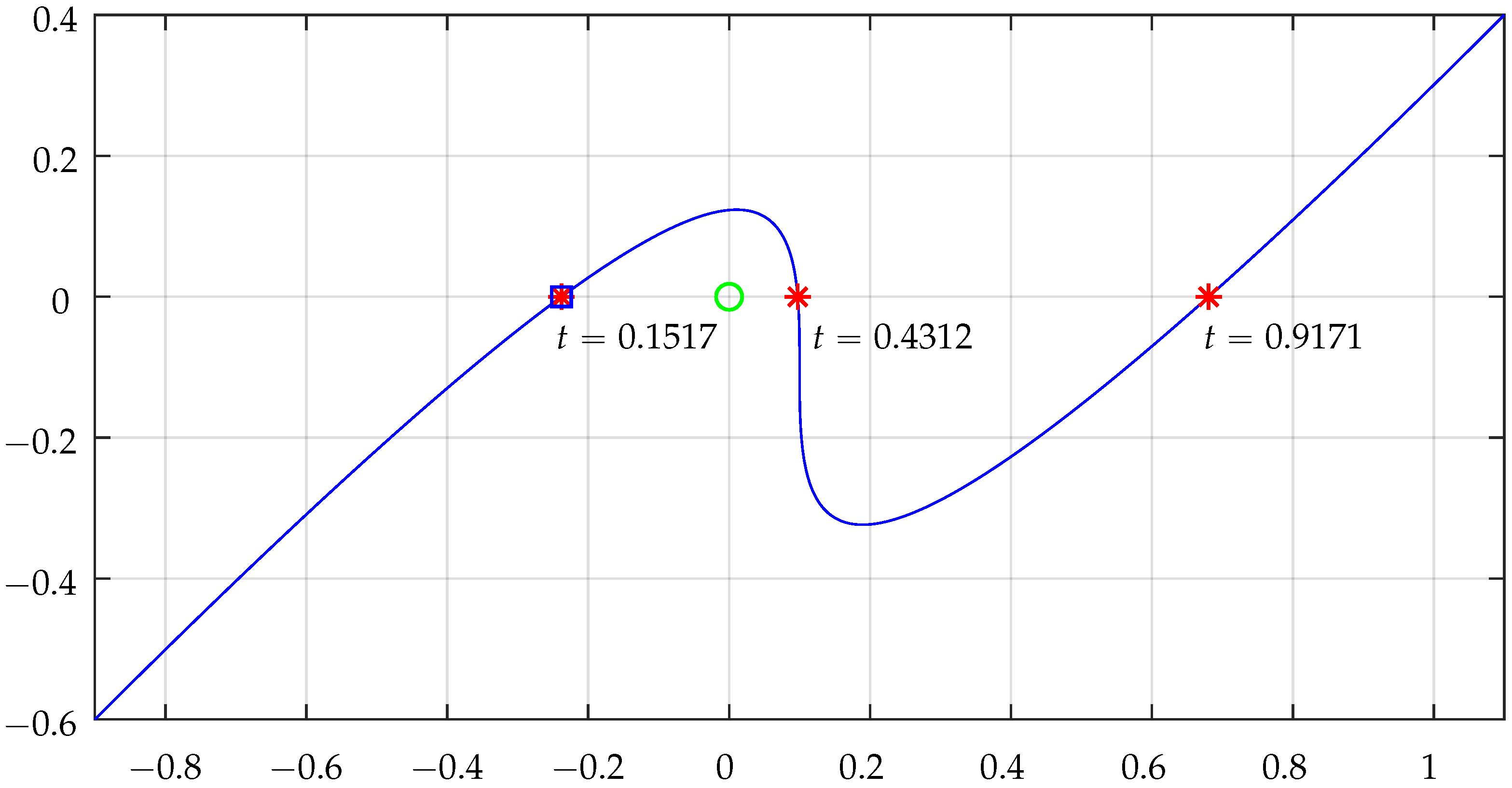
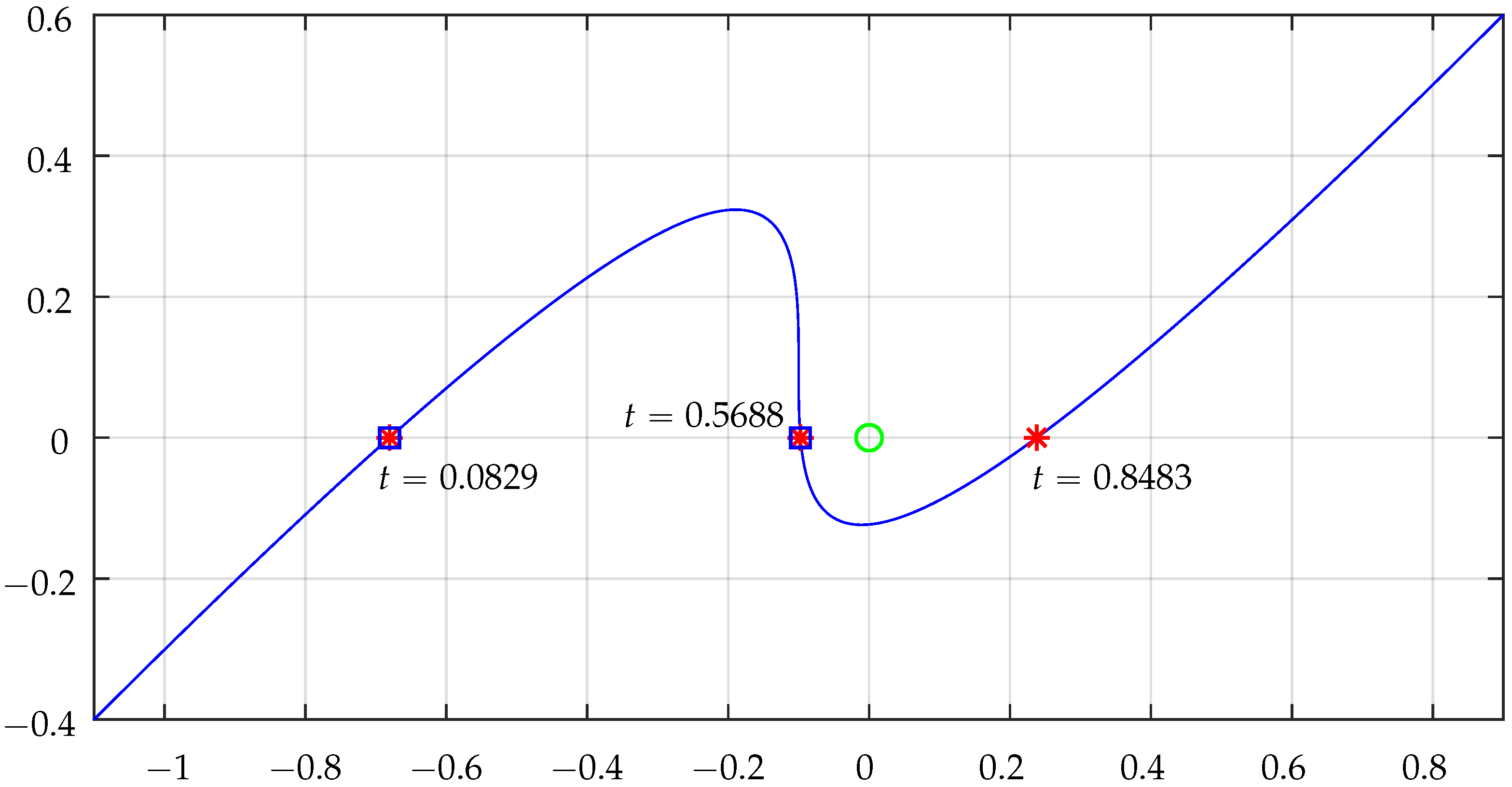
Figure 16 shows a region defined by a cubic Bézier curve and two linear segments. In this case, the Bézier anchor points are
and
and the two control points are
and
. The two linear segments are
and
. Points
and
will be tested but only
is included in the region.
To test points and , the procedure seems to require the adjustment of the “vertices” values reported to each testing point and calculate the new resulting polynomials. Actually, that turns out unnecessary in the parametric form because the new polynomial only changes by an offset, and the generic expression (63) simply becomes , where is the point being tested.
An additional relevant aspect for computational purposes is that the expression for the Bézier polynomial derivative (64) remains the same whatever the testing point
, which saves computation resources when testing the inclusion of many different points for the same region. The generic equations to test the NRA crossing and contributions (
) for a given
are:
To solve the problem for this particular situation, the procedure is implemented as follows:
Find the roots of ;
Test whether the found roots satisfy the condition of NRA intersection, that is, ;
For each root that satisfies the previous expression there is a NRA intersection whose sense needs to be assessed by the sign of .
Table 2 shows some numerical results that illustrate the functionality of the algorithm for a cubic Bézier segment for two test points
and
.
Figure 17 and
Figure 18 illustrate the plots concerning NRA intersections by the cubic Bézier segment for the cases of point
and
, respectively.
The intersection contributions
(detailed in
Table 2) clearly translate the situations of inclusion of the tested points. For
, total
is
and for
total
is
. Actually, the
contributions from the two linear segments were not analyzed, but it is simple to confirm that they do not contribute at all because they do not cross the NRA: the horizontal segment will never contribute, and the vertical segment does not cross the NRA for the points being tested.
With higher order curves, such as these 3rd order Bézier, it may happen that the intersection point is tangent to the NRA and expression (43) would result in 0 (inconclusive). This is an easy situation to detect (one further comparison) and concerns a case where all three roots are equal. There are two solutions for that very special case to allow the detection of the intersection sense: one would be to calculate expression (43) in a “small” neighborhood of , for example, instead of (where the value of can be on the range of the precision involved—e.g., 10−6); the other solution, formally more elegant, is simply to check the quadrants of and , i.e., use the value of .
Application to the Challenges Given
By using the previous techniques for linear, circular, and Bézier segments in an integrated and complementary form, it is possible to test situations as those illustrated in
Figure 1 for a set of random points, which results as shown in
Figure 19.
From the point of view of programming, three functions were created and used: NRAintLin(), NRAintArc() and NRAintBez(), whose source code is also available at the GitHub repository indicated earlier. These functions return the NRA counting for each respective segment when invoked accordingly to the type of segment: 3 linear and 3 circular arcs on the region on the left, and 2 linear, 3 circular arcs and 2 Bézier segments on the region on the right. These three functions are essential to establish the general algorithm for regions delimited by linear, circular, or Bézier segments, which is the subject of the next section.
8. Algorithm for Arbitrary Planar Domains
After the statements, demonstrations, and examples described in the previous sections, it is now straightforward to establish the basis of a general algorithm for arbitrary planar domains that can be described by parametric equations, which have associated a sense of circulation along the boundary. The procedure can be stated as follows:
Set up the closed region by segments defined parametrically in such a way that each segment is defined by two extremes and , a parameter t, being , and optional points or parameters depending on the type of the segments (linear, circular arcs, Bézier curves, etc.)
Linear segments do not require any further parameters or points;
Circular arcs require a third point (center), or else a radius along with the definition of its orientation;
Other curves (of second or higher order) require additional elements to fully define them (3rd order Bézier curves require two more points).
Normalize the domain delimiting points (vertices) relative positions by subtracting the test point a to all vertices.
Check the intersections of this newly relocated region with the negative half part of the horizontal axis (x). Intersections occur from to or vice-versa.
Full intersections are accounted for an integer value (
or
, depending on the sense,
to
(
![Algorithms 17 00444 i019 Algorithms 17 00444 i019]()
) or
to
(
![Algorithms 17 00444 i020 Algorithms 17 00444 i020]()
), respectively), or a partial value (
or
) if the segment starts or ends on the very horizontal axis (
![Algorithms 17 00444 i021 Algorithms 17 00444 i021]()
,
![Algorithms 17 00444 i022 Algorithms 17 00444 i022]()
), and the positive or negative contribution is determined once again if the segment goes or comes to/from quadrants
or
.
The verification of the sense of the evolution of the path must be asserted in these intersection/touching points: it is straightforward for linear segments, but for other types of segments, the descendant gradient of y with respect to t must be used at that point to determine the sense of cross/approach to the horizontal axis.
Algorithm 5 formalizes the required steps
| Algorithm 5: Universal inclusion test in arbitrary regions |
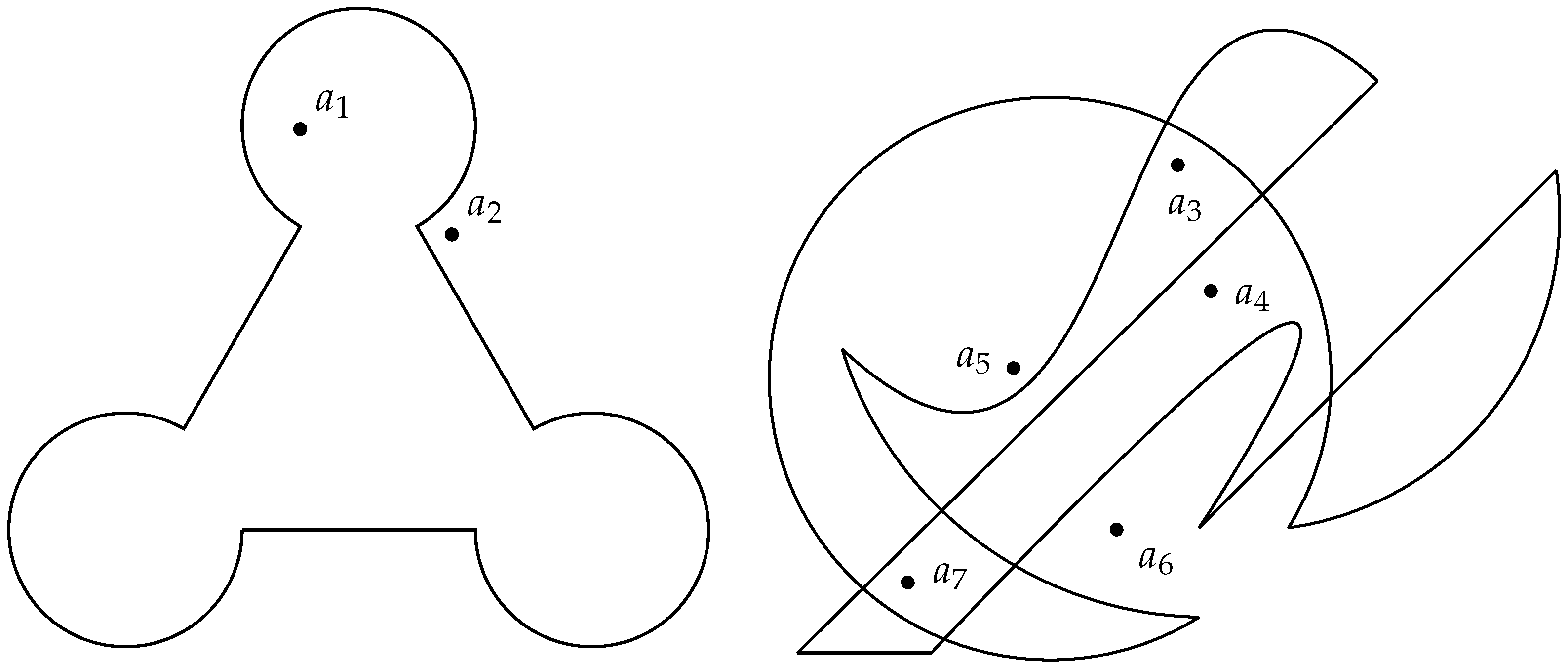
![Algorithms 17 00444 i009a Algorithms 17 00444 i009a]() ![Algorithms 17 00444 i009b Algorithms 17 00444 i009b]() |
A most relevant point when comparing this general algorithm to the algorithms presented in the preceding sections is the input of data: besides the testing point and the list of vertices that require no changes at all, there are now more parameters to be given to distinguish and define the types of segments.
The algorithm then requires the following data as inputs:
The testing point a (same as before)
The vertices (extreme points) of the region segments (same as before)
A set of numbers indicating the type of segment or number of control points (e.g., 0 for linear, 1 for circular, 2 for 3rd order Bézier segments, etc.)
A set of control points for each segment
The steps of the algorithm that vary with the type of segment occur mainly in lines 8 and 9, where the parametric equations of the segment must be obtained and solved, and also in line 15 to calculate a derivative and obtain the sense of NRA crossing.
As mentioned before, the GitHub repository made available also includes the code and illustration of the application of this general algorithm with several examples besides the ones in
Figure 19. No benchmarking is performed with this general algorithm because, in the literature, there are no other algorithms for this same purpose to compare with.
9. Discussion and Conclusions
This paper presents a methodology to solve, in analytical form, the problem of point inclusion in planar domains for regions of virtually unlimited complexity, namely with boundary curves of order greater than linear segments. Specifically, for the cases for regions bounded arbitrarily by polygonal, circular arcs and Bézier lines have been derived and implemented, and the methodology for regions with other shapes has been described and is ready to be applied to the general algorithm.
The approaches described are handled in analytical form, so they are independent of any numerical approximations, hence independent of scale. Nonetheless, when performing actual calculations in floating point operations, the limitation of the numeric representation of the computational system naturally occurs. However, due to the nature of the operations (sums and multiplications in the Algorithms 3 and 4 for polygonal regions only), the propagation of uncertainty is minimal, and operations can even be performed in integer representation, which is suitable for some embedded systems. On the other hand, this is not the case for the general approach of non-linear segments (covered in Algorithm 5) because boundary segments are non-linear, and non-linear calculations are required, including trigonometric or root operations. Since the accumulated chain of non-linear operations is short, uncertainty propagation is contained, and results have shown that very good accuracy (in 12 or more decimal places) is kept in the final outcome. This can be checked, for example, by “zooming” into the plots extensively and verifying the correct result of point inclusion. The mentioned GitHub repository allows these tests to be performed by other users.
The paper also demonstrates why a simple winding number based technique for detecting point inclusion will always be ambiguous if the testing point is on the border. Nonetheless, the proposed algorithms detect those situations early, and the technique relies on the need of a single pass operation, i.e., it requires no iterative procedure or further verifications.
Besides this advantage of a single operation, the possibility of extending the algorithm to regions of more complex shapes opens wider directions in the field of simulation and computational geometry. The usage for curves of high orders needs to deal with negative real axis intersection, which is equivalent to finding the roots of polynomials or other transcendental curves. This implies unavoidable additional computational costs when compared to straight polygonal shapes. Nevertheless, the pure analytical formulation of the method may remain an advantage against the alternatives of linearization or approximation of curves to polygonal lines.
Along these lines, a final remark is worth mentioning, which concerns a potential alternative to this approach for general shapes. We could think of the possibility of triangulating a region such as the ones shown in
Figure 19 and apply point location techniques cited in
Section 2. Although the technique is usually applied for a problem not addressed in this paper, a region could be triangulated and the test of inclusion of a point in the overall region could be performed by identifying which subregion, if any, includes that point. Besides the variable computational costs of this extreme solution, two main limitations immediately arise. The first is concerning self-intersecting regions and regions with holes (like the ones in
Figure 10) that require additional care and pre-processing to be triangulated. Secondly, and even more relevant, if the region boundaries are curved, they must be linearized (sampled) to perform the triangulation. This has two drawbacks: the computational demands of the preprocessing and an additional computational cost that depends on the scale. The dependency on scale is particularly relevant near the boundaries: if very high accuracy is required, the samples over the curved boundaries must be more dense; hence, a larger number of triangles is generated in the mesh. This dependency on scale (with consequences on the accuracy in areas closer to the borders) does not occur in the proposed approach because it is analytical.
The next list of topics explains the advantages of the proposed approach in this paper, the reasons for better performance than existing solutions, and the reason for that to happen.
It involves fewer operations: besides the common sums and subtractions, at most only one floating point division is required per segment (or two multiplications instead) and also fewer comparisons, for the case of polygonal shaped regions. This makes it faster than state of the art solutions (about 5 times as fast was demonstrated for polygons with many sides and a large number of data points for the algorithm implemented in Matlab [
8]).
It has no restrictions on which points define the polygons (or the generically shaped region) nor on the testing points that can be over the border, or being themselves the very vertices, and no particular post processing or operations are required.
It accepts the geometry of boundary segments to be other than straight lines and is applicable virtually to any type of curve that can be expressed parametrically.
The parametric formulation of the boundary makes it straightforward to define the curve segments and their extremes (anchor points).
The parametric definition is intrinsically associated with the concept of sense or circulation, which allows the detection of the sense of axis intersection, and not only the fact that there are intersections; and the sense of intersection is crucial to obtaining the global winding number.
The parametric description allows a separation of coordinates, making algebraic operations independent, and allows us to overcome limitations in degenerate situations that would occur in two coordinate point representations but do not occur in separate coordinate representations.
Although the formal and analytic procedures for point location in generic planar domains have been fully established and demonstrated in this paper, the future may hold improvements in the computational component of the algorithms for specific curves. This can be true, namely for some curves of very high complexity, as well as for the detection of specific situations of point location relative to those more complex boundaries, in order to accelerate the calculation operations.


 ), we have the first case in (24) which, by using the equality of case 3 from (15), certified by (27), allows to state the following:
 ), we have the second case in (24), which allows us to state the following by using the equality of case 2 from (15), as confirmed by (29):
 or
or  ), there will be a contribution of to the contour integral, or in the NRA crossings counter.
 , that is, there is a contribution of to the intersection counting (), or for the reverse case ( to , or
  ). This can be formalized as:
 or
or  ). In those cases, this means that another segment starts or ends there too! To leave the contributions separate, but allowing them to add up or cancel, for those cases, the intersection contribution calculated above should be halved, that is, a contribution for segments that originate or end on the NRA is to be applied. In other words, each crossing of the NRA can be accounted with , but reaching or leaving it can be accounted as a half-crossing, or . Formally, this can be stated as in (45):
 ), the calculation of the line integral is simple (actually, not necessary in practice) because there are no discontinuities in the process and, in the end, all terms of the closed path will cancel altogether; only the intersections of the path with the NRA will affect contour evaluation or the winding number. Also, notice that horizontal segments () never intersect NRA; they may even lie over it but never actually cross it, so their contribution to the is null, as can be seen in the segment that contains the point in Figure 9.


) or to (
), respectively), or a partial value ( or ) if the segment starts or ends on the very horizontal axis (
,
), and the positive or negative contribution is determined once again if the segment goes or comes to/from quadrants or .
