Efficient Multi-Objective Simulation Metamodeling for Researchers

Abstract

Solving multiple objective optimization problems can be computationally intensive even when experiments can be performed with the help of a simulation model. There are many methodologies that can achieve good tradeoffs between solution quality and resource use. One possibility is using an intermediate “model of a model” (metamodel) built on experimental responses from the underlying simulation model and an optimization heuristic that leverages the metamodel to explore the input space more efficiently. However, determining the best metamodel and optimizer pairing for a specific problem is not directly obvious from the problem itself, and not all domains have experimental answers to this conundrum. This paper introduces a discrete multiple objective simulation metamodeling and optimization methodology that allows algorithmic testing and evaluation of four Metamodel-Optimizer (MO) pairs for different problems. For running our experiments, we have implemented a test environment in R and tested four different MO pairs on four different problem scenarios in the Operations Research domain. The results of our experiments suggest that patterns of relative performance between the four MO pairs tested differ in terms of computational time costs for the four problems studied. With additional integration of problems, metamodels and optimizers, the opportunity to identify ex ante the best MO pair to employ for a general problem can lead to a more profitable use of metamodel optimization.

1. Introduction

A simulation model of a physical and/or social system of interest can unlock useful experimental capabilities [1]. Not only are the costs of simulation experimentation in general much lower than an equivalent series of real-world experiments, but there are also scenarios where the latter are simply unfeasible—for example, if the system does not yet exist. However, there always exists a frontier where computational costs limit viable use cases [2].

An Agent-Based Simulation (ABS) usually features decision-making entities who interact with their environment and, directly or indirectly, with one another. When the decisions of many so-called “agents” are critical to system dynamics, utilizing an ABS approach for extending standard models would be a good option, but also a computationally expensive one.

Complicating problem-solving further, many real-world problems, from designing ships to chemical engineering or saving energy, cannot be neatly simplified into a single objective to be maximized or minimized [3]. If one option performs worse in all objectives compared to another option, the first one is “dominated” and would never be worth picking even when both are feasible. At the same time, it is possible to have two options such that neither dominates the other; in this scenario, the decision between them is external to the optimization that produced the options. A collection of all the non-dominated options is most commonly known as a Pareto front but also as Pareto frontier, and Pareto set [4], and as in the two-option case above, does not allow improvements in any objective(s) without having to suffer a worsening of other objective(s). This presents distinctive challenges [5], in particular, the need to thoroughly explore a greater proportion of the input space to generate a Pareto front [6] compared to the single objective problem.

Fortunately, for many optimization problems, a “model of a model”, commonly referred to as a metamodel, can enable experimentation and thus optimization that is less costly than directly using a simulation model. Metamodels are “a mathematical approximation to the implicit input-output function of a simulation model” [7]. They have been adopted in various domains, and depending on the context are referred to as surrogate models, response surface models, or proxy models. Some domains have a rich literature on the use of metamodels within their context [8], but such findings do not necessarily apply to other domains in terms of the most effective use of a metamodel and optimizer. A more general way to make comparisons is by using benchmark problems [9] which may involve a mathematical function [10], domain-specific models [11] or data sets [12]. However, the issue still remains when moving outside domains or problems that are “similar” to these, which led to some siloing and duplication of effort in terms of optimization research in general [13], although there have been efforts to compile this work in a more practitioner-salient form [14].

1.1. Simulation Optimization

The use of simulation in optimization has a long history of development and deployment, and there are a variety of simulation-capable or focused platforms. AnyLogic [15,16] is a popular choice in Operations Research (OR), and options are available for ABS-focused applications [17]. Platforms with more general capabilities like R [18] can also be employed in this role.

Simulation-optimizer methodologies (also known as simheuristics or metaheuristics [19]) are the most direct way to employ a simulation model and optimizer to solve problems, with packages integrating these components like OptQuest and Witness Optimizer being commercially available [20] and open-source options such as SimOpt [21] enabling more user-driven development.

1.2. Metamodeling

When a good balance is struck between efficient exploration of the input space (“learning” the behavior of the system) and focusing on potential areas of optimization interest, a metamodel allows to minimize the use of any costly simulation model evaluations, as described in the work of [22]. Additionally, techniques reviewed by [23] such as variable screening, dimensionality reduction, and use of multiple metamodels can further extend the legs of metamodels, increasing the number of scenarios where they can be profitably employed.

Similar to simulation optimization, methodologies employing metamodels and comparisons between them exist [24]. However, the points of comparison such as between setups, problem types and domains, or specifics of the simulation models used differ between the observed case studies, making it hard to draw fully generalizable conclusions regarding performance or cost characteristics.

Of course, some domains have long-established and well-explored metamodels. For example, the domain of energy prediction models [25] extends standard surrogate energy prediction models by incorporating household preferences into the underlying simulation model and using an artificial neural network metamodel. In engineering designs, kringing regression is popular, as demonstrated in applications such as vacuum/pressure swing adsorption systems [26]. Polynomial-based surrogates are also seeing advancements in engineering applications [27]. These are not the only options, as metamodeling does not have a “one size fits all” methodology. Technique selection comes with various trade-offs. Ref. [28] compares a number of these trade-offs for the scenario of building design optimization while [29,30] do the same for the water resources modeling case.

There is a growing number of studies on deep learning to fully exploit the power of neural networks. Deep learning has been applied to many real-world problems successfully, however, two main issues, among others, raised by [31] are relevant to consider. First of all, deep learning techniques require a large amount of data. As one of the goals of this work is a methodology that minimizes the use of expensive simulation model evaluation, gathering this data to train a deep learning system would not be ideal. Secondly, deep learning models can have high memory and computational requirements. As a result, while deep learning can provide a high level of flexibility, when simpler metamodels, where the best is selected from a variety of options, can achieve good final Pareto front performance, the approach that requires less data and incurs lower computational costs might be more appropriate.

1.3. Optimizers

Implicit in the above discussion is the need for an optimizer heuristic to decide which experiments to run and at which level of model; evolutionary methodologies [32] like genetic algorithms are a popular choice. The ability to algorithmically test and evaluate various Metamodel Optimizer (MO) pairs would also bring benefits for researchers and practitioners in terms of reproducibility and avoiding reliance on excessive problem- or domain-specific tuning; finely tailored heuristics can exhibit improved performance but with less visible costs of requiring specific knowledge or reducing the generalizability of the solution method, something pointed out by the review of [13].

1.4. Aim

The aim of this paper is to introduce a comprehensive methodology designed to facilitate the systematic application and evaluation of metamodeling and optimization heuristics. While platforms exist to handle setups utilizing metamodels, such as OPTIMIZE [33], these focus more on enabling users without specialist optimization knowledge to employ metamodeling to solve optimization problems. In contrast, our methodology enables researchers to compare setups experimentally, determining which MO pair is the best performer at each tested time limit for a given problem, in a way that allows drawing specific and in some cases general conclusions about the optimal MO pairs.

2. Test Environment and Methods

The primary feature of the test environment is to enable researchers to run experiments on discrete multiple objective optimization problems using a simulation model and metamodel. These experiments evaluate the relative performance of MO pairs on a time and solution quality basis. As many such experiments may need to be conducted and the main goal of employing a metamodel is to economize on simulation model costs, the test environment utilizes a specific method for generating and storing simulation model Full Evaluations (FEs), or FE, for all future users. For each problem, corresponding to a simulation model, an exhaustive list of input–output data (including evaluation times) allows for faster-than-FE lookup, and reproducible FEs. In addition, this mechanism takes a stochastic simulation model and provides all future users with a deterministic response to any set of inputs, namely the mean of the simulation repetitions for that specific set of inputs.

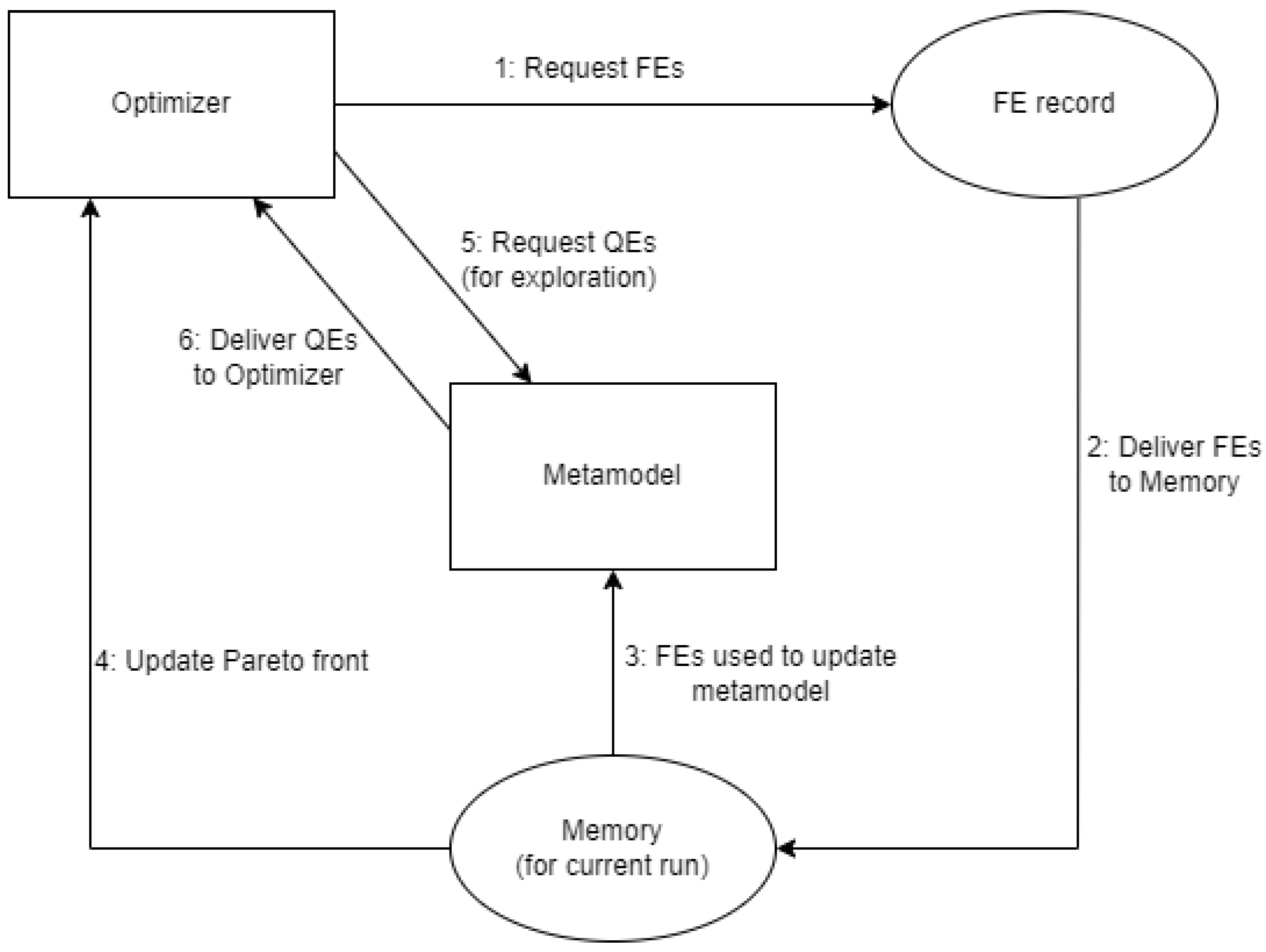
The components of the test environment interact as illustrated in Figure 1. Notably, while the external simulation models are evaluated on another platform (AnyLogic or SimOpt), users will use the FE record, meaning that only R needs to be actively executed for experiments. This record is separate from what the optimizer has in “memory” for each experiment run, which only consists of FEs it has already requested and “paid for” in terms of time costs and any Quick Evaluations (QEs) it has made via the latest updated metamodel.

The overall sequence followed to complete an experiment run is as follows:

• Optimizer requests FEs;
• Requested FEs are delivered to memory;
• All FEs in memory are used to update the metamodel;
• Optimizer updates its current Pareto front, using all FEs in memory;
• Optimizer requests QEs from metamodel (this is an exploration step);
• Metamodel delivers QEs to the optimizer;
• If any of the QEs would be part of the Pareto front, they will be listed and requested by returning to step 1.

For each experiment run, the first time step 1 occurs, the FEs requested correspond to the initial sample. Step 4 can be considered the exploitation step each time it occurs except the first time, as this is when the Pareto front actually improves. Although QEs are used to identify potential additions to the Pareto front, the objective values from a QE must be “confirmed” with FEs for those inputs.

If an experiment run reaches the time limit while going through a list of requested FEs, only the FEs that would have been done before the time limit can be part of the final Pareto front. Otherwise, reaching the time limit means that the most recent Pareto front is the one that is stored and evaluated.

For each problem investigated, a set of experiments is run on the simulation model, using different combinations of metamodel, optimizer and time limits. Each experiment run produces a Pareto front as output, which will be stored for later use. Once the experiment is completed, all Pareto fronts can be evaluated using the metrics detailed below. This allows the user to compare the evolution of solution quality against the time limit for each MO pair.

2.1. Metamodels

Two different popular metamodeling methodologies are integrated into the test environment. The first is based on Gaussian regressions, and the second is using a neural network approach. It should be noted that the solution Pareto fronts will only contain points that have been obtained through FE.

2.1.1. Gaussian Regression (GR) Metamodel

This metamodel employs the “GPFDA” package (https://github.com/gpfda/GPFDA-dev, accessed on 23 May 2023) for R [34] and treats outputs as independent, though this is not a restriction on all Gaussian regressions.

For an objective x, the FEs in memory relate values of the objective to values of the inputs, so if there are n FEs in memory, we can express $Memory=\{(x_1,t_1),(x_2,t_2),\dots (x_n,t_n)\}$ where $t_j$ is a vector of input values corresponding to $x_j$.

The Gaussian regression model for x is then:

$$\begin{array}{cc}\hfill x_i& =f\left(t_i\right)+{ϵ}_i,i=1,\dots ,n\hfill \\ \hfill e_i& \sim i.i.d.N(0,{\sigma }_{ϵ}^2)\hfill \\ \hfill f(.)& \sim GP(\mu (.),k(.,.))wherek(t_i,t_j)=COV(f\left(t_i\right),f\left(t_j\right))\hfill \end{array}$$

(1)

The mean function used is $\mu (.)=0$, which means the covariance function of a Gaussian process is the only item that has to be estimated in order to characterize that Gaussian process.

The Matern covariance function is used here, so:

$$\begin{array}{cc}\hfill k(t_i,t_j)& =v_0\frac{{\left(d\sqrt{2\nu }\right)}^{\nu }}{\mathsf{\Gamma }\left(\nu \right)2^{\nu -1}}{K}_{\nu }\left(d\sqrt{2\nu }\right)\hfill \\ \hfill d& =|t_i-t_j{|}^2\hfill \end{array}$$

(2)

where $K_{\nu }$ is the modified Bessel function of order $\nu$, and $\nu =1.5$ is used.

2.1.2. Neural Network (NN) Metamodel

This metamodel employs the “neuralnet” package (https://github.com/bips-hb/neuralnet, accessed on 23 May 2023) for R [35] and uses a back propagation algorithm. Specifically, the neural network used here consists of input neurons $x_{IN,1},x_{IN,2},\dots ,x_{IN,n_{IN}}$ corresponding to the inputs, output neurons $x_{OUT,1},x_{OUT,2},\dots ,x_{OUT,n_{OUT}}$ corresponding to the number of objectives, and $n_H$ layers of hidden neurons, where $x_{i,j}$ correspond to the jth neuron on the ith hidden layer. Input neurons interact only with neurons on the first hidden layer, and neurons on each hidden layer interact only with neurons on the following hidden layer, with neurons on the final hidden layer interacting with the output neurons.

As a result, in a system with $N_H$ hidden layers, where the ith hidden layer has $n_i$ neurons, the value of the first output neuron (dropping the $OUT,1$ notation for clarity) might be expressed as:

$$x=f(w_0+\sum _{j=1}^{n_{N_H}}{w}_j\ast x_{N_H}).$$

(3)

Every neuron has a weight for each neuron on the previous layer, and a constant neuron. The weighted sum of neuron values on the previous layer (for output neurons, the previous layer is the $N_H$th hidden layer) is the input to $f\left(\right)$, the activation function. In this case, the activation function is the logistic function: $f\left(u\right)=\frac{1}{1+e^{-u}}$ as it gives final outputs in the interval $[0,1]$ and the metamodel works on inputs and objectives scaled to this interval.

In keeping with the design intent to minimally adjust component settings, the main default options are used for training the model. In particular, the algorithm used is the resilient backpropagation with weight backtracking by [36] on two layers of hidden neurons (five in the first layer and three in the second).

2.2. Optimizers

The two implemented optimizers make use of a metamodel to explore potential solutions before deciding which ones to request FEs for. At the start of each run, the optimizer starts off with no FEs and thus cannot train a metamodel. This is why the first step for all optimizers is to draw an initial sample of FEs from the input space in proportion to its size. For our experiments, the initial sample size is always fixed at 5% of the input space. Other than this initial sample, optimizers only request FEs for solutions that are expected to improve their Pareto front. When the time limit is reached, optimizers will stop and record the Pareto front from all the obtained FEs.

2.2.1. Basic (B) Optimizer

The algorithm is as follows:

• Perform initial sampling;
• Using the list of all prior FEs, train metamodel;
• Populate the full list of candidate solutions by requesting QEs;
• Remove all Pareto-dominated solutions to generate a potential Pareto front;
• If any solutions of the Pareto front are from a QE, request FEs, store the results and return to step 2, else;
• If all solutions on the Pareto front are from FEs, the optimizer terminates successfully.

If step 6 is reached, the optimizer has no FEs to request. This means there is no new data to update the metamodel, and as it already in step 3 used the metamodel exhaustively for QEs, the input space is fully explored. As a result, it will terminate even if the time limit has not yet been reached.

2.2.2. Genetic Algorithm (GA) Optimizer

The algorithm is as follows:

• Perform initial sampling;
• Using the list of all prior FEs, train metamodel;
• Remove all Pareto-dominated solutions to generate a Pareto front—this is the “parent population”;
• Generate new “children” solutions;
• Request QEs for all children solutions;
• Generate a new Pareto front from the combined parents and children population;
• If any solutions of the Pareto front are from a QE, request FEs, store the results and return to step 2, else;
• If all solutions on the Pareto front are from FEs, return to step 4.

The population for the genetic algorithm consists of all solutions on the Pareto front. These always consist of FEs. Children are generated by randomly selecting two parent individuals at random. Each time step 4 occurs, up to twice the number of the parent population or the number of the initial sample size (whichever is greater) of children will be generated.

There is a 10% chance for each input to undergo crossover, and a 10% chance for each input to mutate by 1, subject to input constraints. In step 8, all “children” from the previous step 4 become part of the next “parent” generation. This optimizer always utilizes the full allowed time limit, even if it constantly generates new “children” that do not meet expected improvements.

2.2.3. Normalized Hypervolume

The hypervolume measure is calculated by defining a section of the problem’s output space bounded by each objective’s minimum and maximum as observed from the optimal Pareto front, the set $A\subset {\mathbb{R}}^d$ (d is the number of objectives). Any Pareto front is a set of points, B, with each point $b\in B$ dominating a portion of A, the set $D(b,A)\subset A$. The hypervolume of the Pareto front B is thus:

$$H{V}_B=\mathsf{\Lambda }\left({\cup }_{b\in B}D(b,A)\right)$$

(4)

where $\mathsf{\Lambda }$ is the Lebesgue measure.

The hypervolume measure is normalized by dividing the hypervolume of a Pareto front by the hypervolume of the optimal Pareto front. The maximum is 1. Thus, a higher normalized hypervolume indicates a better-quality solution.

2.2.4. Normalized Hausdorff Distance

The Hausdorff distance [37] measures how close two sets are to each other. For finite sets (which the Pareto fronts here all are due to the discrete problem construction) the Hausdorff distance between sets X and Y can be expressed as:

$$dis{t}_H=max[\underset{x\in X}{max}d(x,Y),\underset{y\in Y}{max}d(y,X)]$$

(5)

where $d(a,B)$ is the minimum Euclidean distance between a point a and any member of set B. The Hausdorff distance is normalized by dividing the Hausdorff distance between a Pareto front and the optimal Pareto front by the maximum Hausdorff distance between any Pareto front from the experiment set and the optimal Pareto front. The minimum (between a set and itself) is 0. Thus a lower normalized Hausdorff distance indicates a better-quality solution.

2.2.5. Normalized Crowding Distance

The crowding distance [38] measures how close points on a Pareto front are to each other. In the case where there are $N_o$ objectives and $N_p$ Points on the Pareto front, every point on the Pareto front will have a series of rankings $(x_1,x_2,\dots x_j,\dots x_{N_o})$ where each $x_j$ is its ranking in objective j ($x_j\in [1,2\dots N_p]$). Let $I\left[a\right].b,b\in [1,2\dots N_o]$ denote the objective value of element a in the ranking corresponding to objective b.

For every non-boundary point (not at the maximum or minimum for any one objective as observed on the Pareto front) with the per-objective rankings as above, we can define its crowding distance as:

$$C{D}_{point}=\sum _{j=1}^{N_o}\frac{I[x_j+1]·j-I[x_j-1]·j}{ma{x}_j-mi{n}_j}$$

(6)

where $ma{x}_j$ and $mi{n}_j$ are the maximum and minimum values for objective j.

The crowding distance for the whole Pareto front is then calculated as the average of the crowding distances across all non-boundary points. The crowding distance is normalized by dividing the crowding distance of a Pareto front by the crowding distance of the optimal Pareto front. A lower normalized crowding distance implies points on the Pareto front are closer to one another, which indicates a better-quality solution.

3. Experimentation

3.1. Simulation Models

For our experimentation, we have chosen four OR simulation models as part of the test environment, which are deployed together with the FE records in the Supplementary Material: A student services model and a telecom model [39] models—which were run in AnyLogic as well as a Continuous News Vendor model and a dual sourcing model [21], which run in the Python-based SimOpt package (https://pypi.org/project/simoptlib/, accessed on 23 May 2023).

3.1.1. Student Services Simulation

This model represents a trio of student service centers that face a stochastic distribution of incoming students in each location. These students require different types of service: one general service and two specific services. The two objectives being examined are the total labor costs of hiring three different classes of employees corresponding to service types (specialists can handle their specific specialist enquiries as well as general enquiries, while non-specialists can only handle general enquiries) and the total time cost, faced by students on average.

The student traveling, queuing and service processes correspond to a classic discrete event simulation with stochastic elements, while the simulation model’s main agent-based features are the students, using a “smart app” that gives students information about queue length and average waiting times, allowing them the decision to select between different centers. A student using the smart app will select the service center with the lowest expected time cost to them, considering not only the expected queuing times but also travel time, which depends on the distance of the student from a service center as well as the student’s travel speed.

Students start in one of three locations, with each location being close to one service center (5 distance units away) and far from the other two service centers (15 distance units away). The distribution of student starting locations is not uniform each day, but instead one service center will see half of the students starting near it, and the other two service centers will see one quarter of the students starting near each of them. Students have stochastic travel speeds, with a mean of one distance unit per minute. Even with the smart app, students do not know the exact time they will be queuing at the time they start, but this is estimated by multiplying a moving average of waiting times for their enquiry type by the queue length for their enquiry type at the time they make their decision. The expected service time after traveling and queuing is the same across all centers for any given student enquiry type (which they are aware of).

3.1.2. Telecom Simulation

This model is a publicly available AnyLogic example model [39] of a telecom company operating in a market with competitors. The inputs of interest are call price per minute and aggressiveness (referring to marketing effectiveness). The objectives of interest are as follows: voice revenue (which is specific to people paying to make calls), “value added” service revenue (which covers other items besides calls), as well as aggressiveness itself, as the cost of the required marketing strategy to reach a certain level of effectiveness is not represented within the model. In this model, aggressiveness affects the addressable market share, but users decide which company to support based on the prices they observe. This behavior is implemented in the model by referencing tables that presumably represent statistical market research on the probabilities involved.

The Telecom simulation allows for dynamic adjustment of the inputs, which will result in a transition to a new market equilibrium. For the case study, selected inputs were applied at the start of the simulation. The experimental inputs do not correspond to the initial market state. This requires the simulation to be run until it reaches the new equilibrium, at which time the objectives can be measured.

3.1.3. Continuous News Vendor Simulation

This model is included in the SimOpt distribution and represents a newsvendor who orders a quantity of stock, and decides on a price to sell it to customers. However, the day’s demand is randomly drawn from a Burr Type XII distribution, where the cumulative distribution is given by:

$$F\left(x\right)=1-{(1+x^{\alpha })}^{-\beta }$$

(7)

with $\alpha =2$ and $\beta =20$.

The two inputs of interest relate to stock quantity and selling price decisions, while the two objectives of interest are the news vendor’s profits and the quantity of stock actually sold.

3.1.4. Dual Sourcing Simulation

This model is included in the SimOpt distribution and represents a manufacturing location purchasing its input via regular or expedited suppliers with different ordering costs and delays while facing stochastic demand. Regular deliveries cost 100 per unit and take 2 days to arrive, while expedited deliveries cost 110 per unit but take 0 days to arrive. One simulation run will simulate 1000 days of operation.

There are storage costs when the location carries stock from one day to the next day, and a penalty “cost” per unit of shortage whenever there is a lack of stock to meet demand. Satisfied demand has no benefit other than zero penalty, which implies that location is a substitute for a cost center that aims to minimize costs and penalties.

The strategy followed by the location can be summarized as follows: It consists of having two inventory target levels, one for the regular supplier and one for the expedited supplier. The location will place an order with a specific supplier whenever the stock level falls below its associated threshold value. Although the goods being ordered are homogeneous when in stock, goods that are yet to arrive are not considered against the target level for the expedited supplier as they will only arrive after the expedited delivery.

The two inputs of interest are these two threshold levels. The three objectives of interest are the three main types of costs to be considered: ordering costs, holding costs and penalties for running out of stock.

3.2. Procedural Steps

We compare the performance of MO pairs on each simulation model separately, as each such case study corresponds to a different scenario. There are four scenarios in total. Each case study used four time limits, so from an optimization standpoint, there are four problem instances per case study, for sixteen total across all case studies. Each individual experiment specification is run fifty times with the same setup, as is required for stochastic experimentation.

More specifically, each case study covers all possible combinations of the following:

• Two metamodel options (Gaussian regression, Neural network);
• Two optimizer options (Basic, Genetic algorithm);
• Four time limits (as determined for each simulation problem).

The selection of time limits is different for each simulation model. The lowest time limit corresponds to the time required to carry out the FEs corresponding to the initial sample. For all experiments, initial sample sizes are 5% of the simulation model’s input space, although this can be user-defined. The initial sample is uniformly and randomly distributed via Latin hypercube sampling.

The experiments are run sequentially, from the initial sampling until the time limit is reached or, for the Basic optimizer only, if the stopping condition is reached before the time limit. As the test environment uses FE records instead of obtaining objective values from running the simulation model directly for each required set of inputs, the real-world time taken for an experiment will be shorter than the time limit, as the time limit accounts for the full FE time costs. For each completed experiment, the final Pareto front is stored. All Pareto fronts for a given case study are evaluated as a set, as the metrics used to evaluate MO pair performance are all normalized.

Three metrics, normalized hypervolume, normalized Hausdorff distance and normalized crowding distance, are used to evaluate the obtained Pareto fronts, which, for consistency, use as a reference the Pareto front generated from the exhaustive FE record. This optimal Pareto front, corresponding to the specific simulation model problem, remains the same whenever the simulation model is referenced, ensuring that all metrics have a common benchmark across different sets of experiments.

3.3. System Configuration and General Experimental Setup

All experiments were run on a laptop with a dual-core 11th Gen Intel(R) Core(TM) i5-1135G7 (2.40 GHz, 2.42 GHz) CPU and 20 GB of RAM (Intel, Santa Clara, CA, USA). This same system was used to generate the FE records.

4. Results

When identifying specific MO pairs, the acronyms for metamodels (Gaussian Regression: GR, Neural Network: NN) and optimizers (Basic: B, Genetic Algorithm: GA) are used to identify MO pairs in that order (metamodel optimizer). For example, GR-B corresponds to experiments using the Gaussian regression metamodel and Basic optimizer.

For each of the four time limits, we identified the best-performing MO pair with respect to the mean normalized hypervolume, denoted as ${\mu }_{norm}$, considering each case study. We applied a paired Wilcoxon signed-rank test to determine if the best-performing and each of the other MO pairs have a statistically significant performance difference within a confidence interval of 95%. Table 1, Table 2, Table 3 and Table 4 summarize the results obtained by repeating each experiment for fifty trials, providing ${\mu }_{norm}$ associated with the standard deviation, indicated as $\sigma$- and p-values for each pair-wise statistical performance comparison of the best and associated MO pairs.

Before we come to presenting the individual results, there is one more point to clarify. While one would expect the mean quality of Pareto fronts for a given MO pair to always stagnate or increase with higher time limits, we found that the mean quality in this case sometimes decreases. The explanation for this behavior is that experiments with different specified time limits are not direct “progressions” from one another and there is variance of results, even when individual time limits are higher.

4.1. Student Services Simulation Case Study

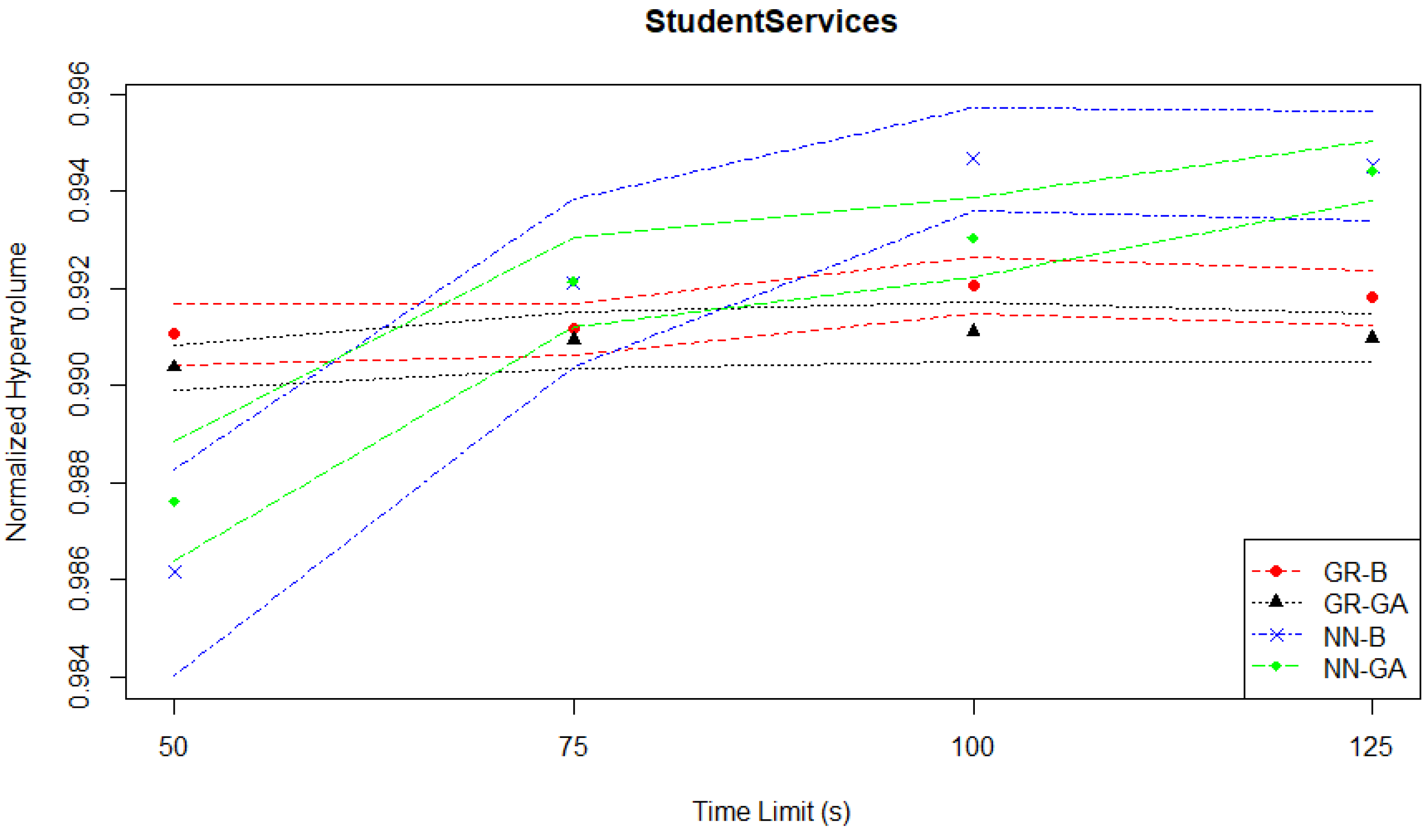
As mentioned in Section 3.1.1, the goal of this case study is to optimize the operations of three student service centers that handle stochastic student arrivals and offer both general and specialized services. Figure 2 shows the relationship between normalized hypervolume and time limits for the Student Services problem. The symbols between the two lines of each MO pair represent the mean value, while the lines represent the limits of the associated confidence interval. The graph suggests that the Student Services problem is relatively easy to solve, as all MO pairs, even with low time limits, can achieve a high normalized hypervolume (above 0.98).

Table 1 summarizes the results for the Student Services experiments based on the mean normalized hypervolume performance (${\mu }_{norm}$s) of each MO pair with the best-performing one at each time limit. The results show that at the lowest time limit of 50 s, GR-B turns out to be the best-performing approach while GR-GA delivers a similar performance based on the statistical test. As the time limit is increased to 75 s, NN-GA becomes the best approach, where the performance difference is statistically significant with p-values being less than 0.05 when compared to both GR-based methods. NN-B delivers a similar, but slightly worse performance than NN-GA. As the computational budget is increased further to 100 s and 125 s, NN-B outperforms the other MO pairs, while NN-GA ranks the second best method with a similar performance to NN-B, except for 100 s. The GR-B and GR-GA pairs once again turn out to be the worst methods of all. The performance difference between NN-B and GR-based methods is statistically significant at the 95% confidence level for the time limits greater than 50 s. Regardless of the given time limit, all methods produce a ${\mu }_{norm}$ about 0.99.

Table 1. Student services experiments—normalized hypervolume performance comparison of each MO pair with the best-performing one at each time limit.

Time Limit (s)	MO Pair	${\mathit{\mu }}_{\mathit{norm}}$	$\mathit{\sigma }$	p-Value
50	GR-B	0.991049	3.23 × 10${}^{-4}$	Best
	GR-GA	0.990360	2.35 × 10${}^{-4}$	8.61 × 10${}^{-2}$
	NN-B	0.986146	1.08 × 10${}^{-3}$	1.57 × 10${}^{-4}$
	NN-GA	0.987603	6.28 × 10${}^{-4}$	1.37 × 10${}^{-5}$
75	GR-B	0.991151	2.71 × 10${}^{-4}$	3.76 × 10${}^{-2}$
	GR-GA	0.990927	2.88 × 10${}^{-4}$	8.04 × 10${}^{-3}$
	NN-B	0.992102	8.78 × 10${}^{-4}$	3.97 × 10${}^{-1}$
	NN-GA	0.992128	4.74 × 10${}^{-4}$	Best
100	GR-B	0.992058	2.95 × 10${}^{-4}$	1.93 × 10${}^{-5}$
	GR-GA	0.991106	3.16 × 10${}^{-4}$	1.94 × 10${}^{-6}$
	NN-B	0.994665	5.34 × 10${}^{-4}$	Best
	NN-GA	0.993041	4.19 × 10${}^{-4}$	4.96 × 10${}^{-3}$
125	GR-B	0.991801	2.92 × 10${}^{-4}$	3.17 × 10${}^{-4}$
	GR-GA	0.990969	2.52 × 10${}^{-4}$	3.94 × 10${}^{-6}$
	NN-B	0.994517	5.65 × 10${}^{-4}$	Best
	NN-GA	0.994415	3.06 × 10${}^{-4}$	1.29 × 10${}^{-1}$

Table 1. Student services experiments—normalized hypervolume performance comparison of each MO pair with the best-performing one at each time limit.

Time Limit (s)	MO Pair	${\mathit{\mu }}_{\mathit{norm}}$	$\mathit{\sigma }$	p-Value
50	GR-B	0.991049	3.23 × 10${}^{-4}$	Best
	GR-GA	0.990360	2.35 × 10${}^{-4}$	8.61 × 10${}^{-2}$
	NN-B	0.986146	1.08 × 10${}^{-3}$	1.57 × 10${}^{-4}$
	NN-GA	0.987603	6.28 × 10${}^{-4}$	1.37 × 10${}^{-5}$
75	GR-B	0.991151	2.71 × 10${}^{-4}$	3.76 × 10${}^{-2}$
	GR-GA	0.990927	2.88 × 10${}^{-4}$	8.04 × 10${}^{-3}$
	NN-B	0.992102	8.78 × 10${}^{-4}$	3.97 × 10${}^{-1}$
	NN-GA	0.992128	4.74 × 10${}^{-4}$	Best
100	GR-B	0.992058	2.95 × 10${}^{-4}$	1.93 × 10${}^{-5}$
	GR-GA	0.991106	3.16 × 10${}^{-4}$	1.94 × 10${}^{-6}$
	NN-B	0.994665	5.34 × 10${}^{-4}$	Best
	NN-GA	0.993041	4.19 × 10${}^{-4}$	4.96 × 10${}^{-3}$
125	GR-B	0.991801	2.92 × 10${}^{-4}$	3.17 × 10${}^{-4}$
	GR-GA	0.990969	2.52 × 10${}^{-4}$	3.94 × 10${}^{-6}$
	NN-B	0.994517	5.65 × 10${}^{-4}$	Best
	NN-GA	0.994415	3.06 × 10${}^{-4}$	1.29 × 10${}^{-1}$

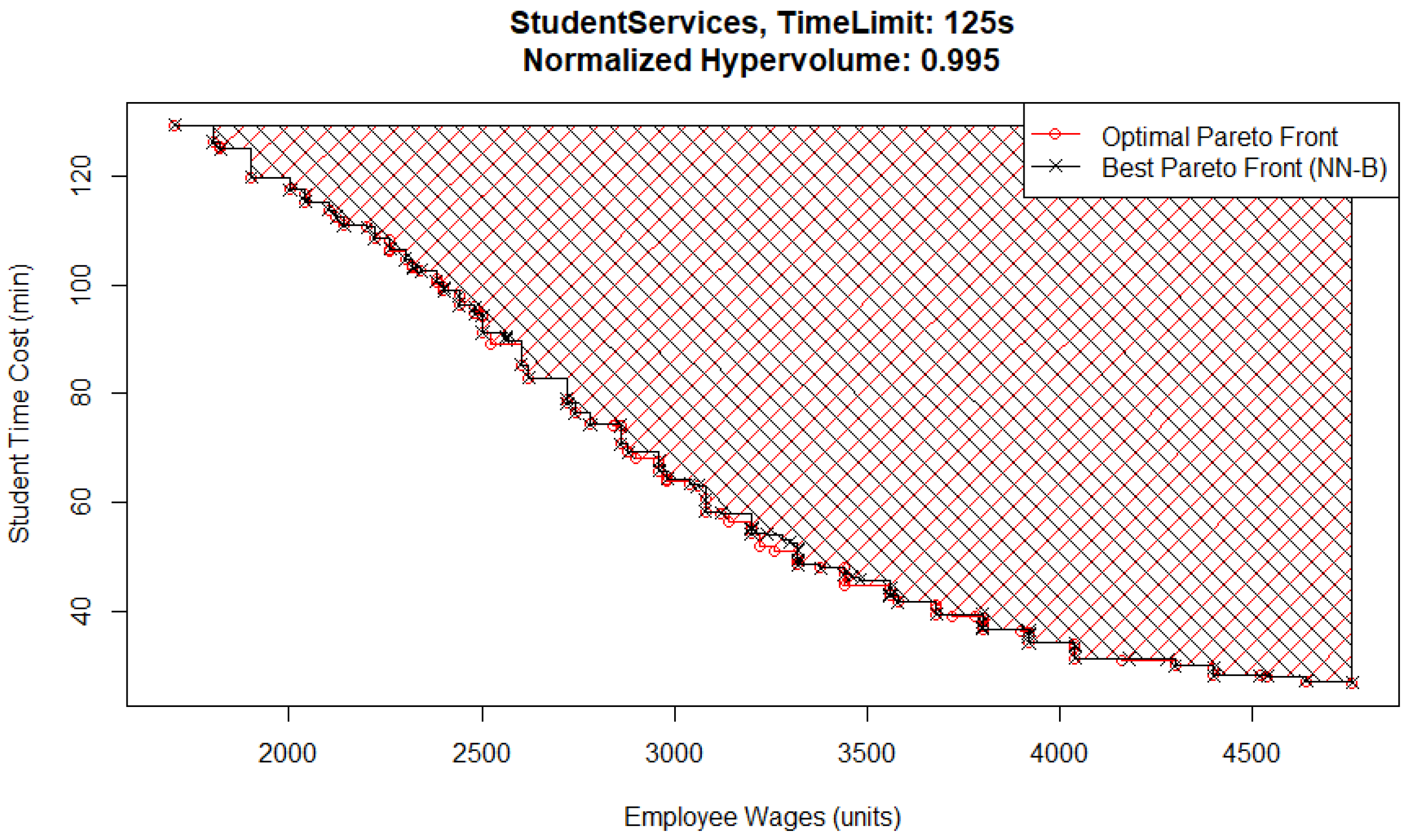
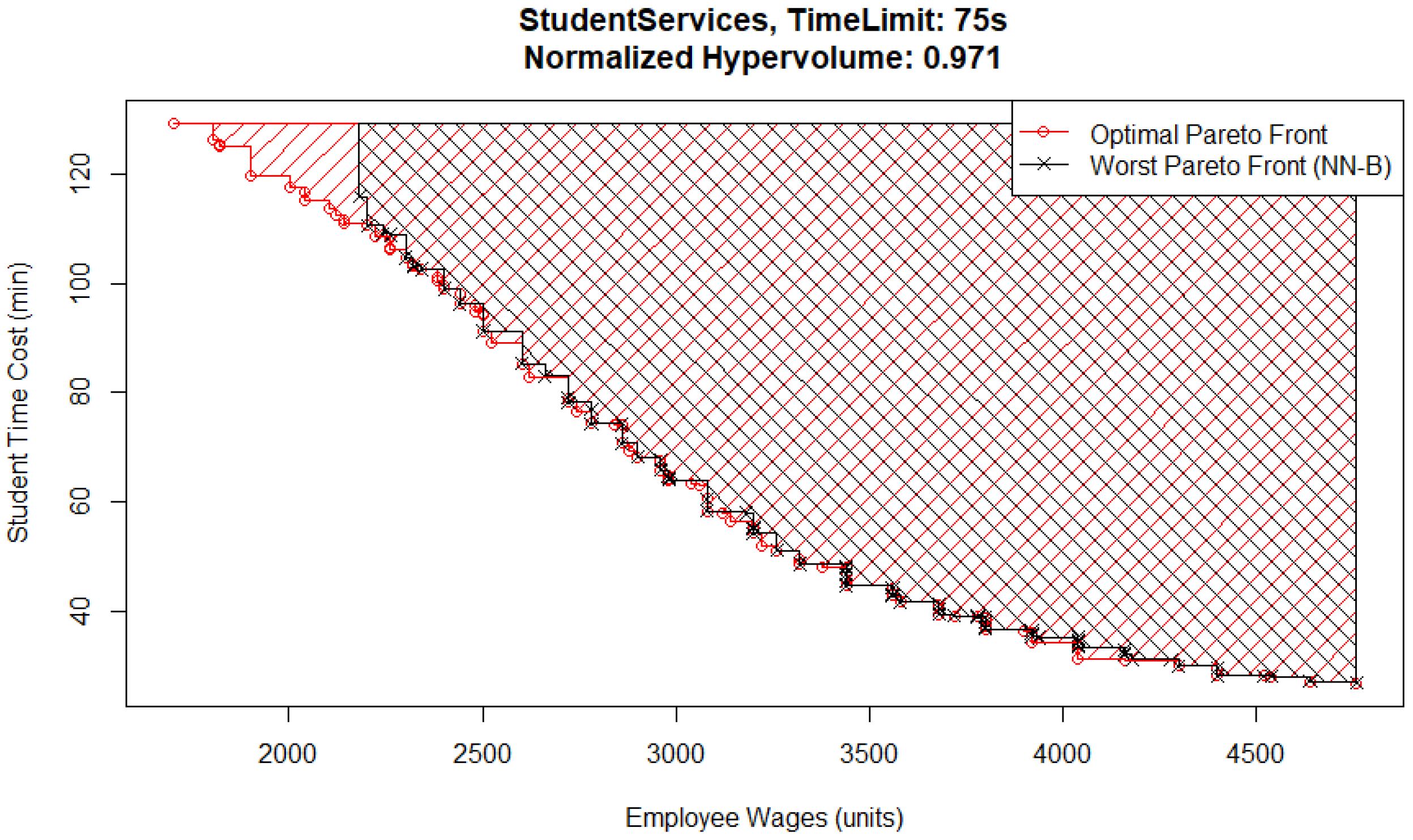
One interesting detail is that for the 75 s time limit case, the best Pareto front (Figure 3) and the worst Pareto front (Figure 4) are both from the NN-B pair, which has the largest standard deviation across all MO pairs and time limits. The reason for the difference between them is that the metamodel in the worst case has underestimated the performance of solutions that would have otherwise been located in the top left corner of the Pareto front, where wages are low and student inquiry time is high. In this case, that means it had an excessively high estimate for student time cost or employee wages. The explanation for this is that the Basic optimizer uses the metamodel evaluations to check every possible solution and does not identify them as possible candidates for inclusion.

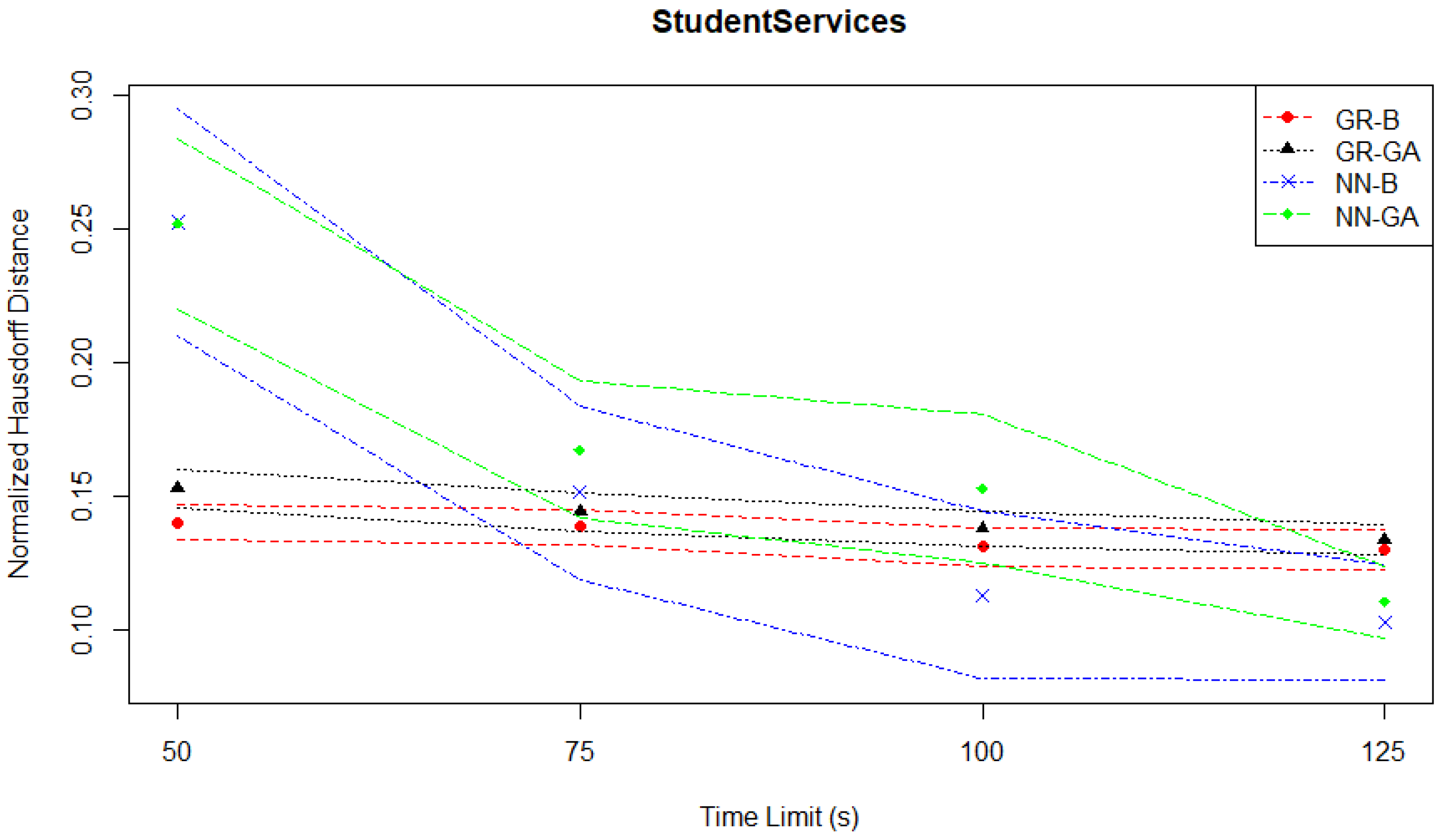
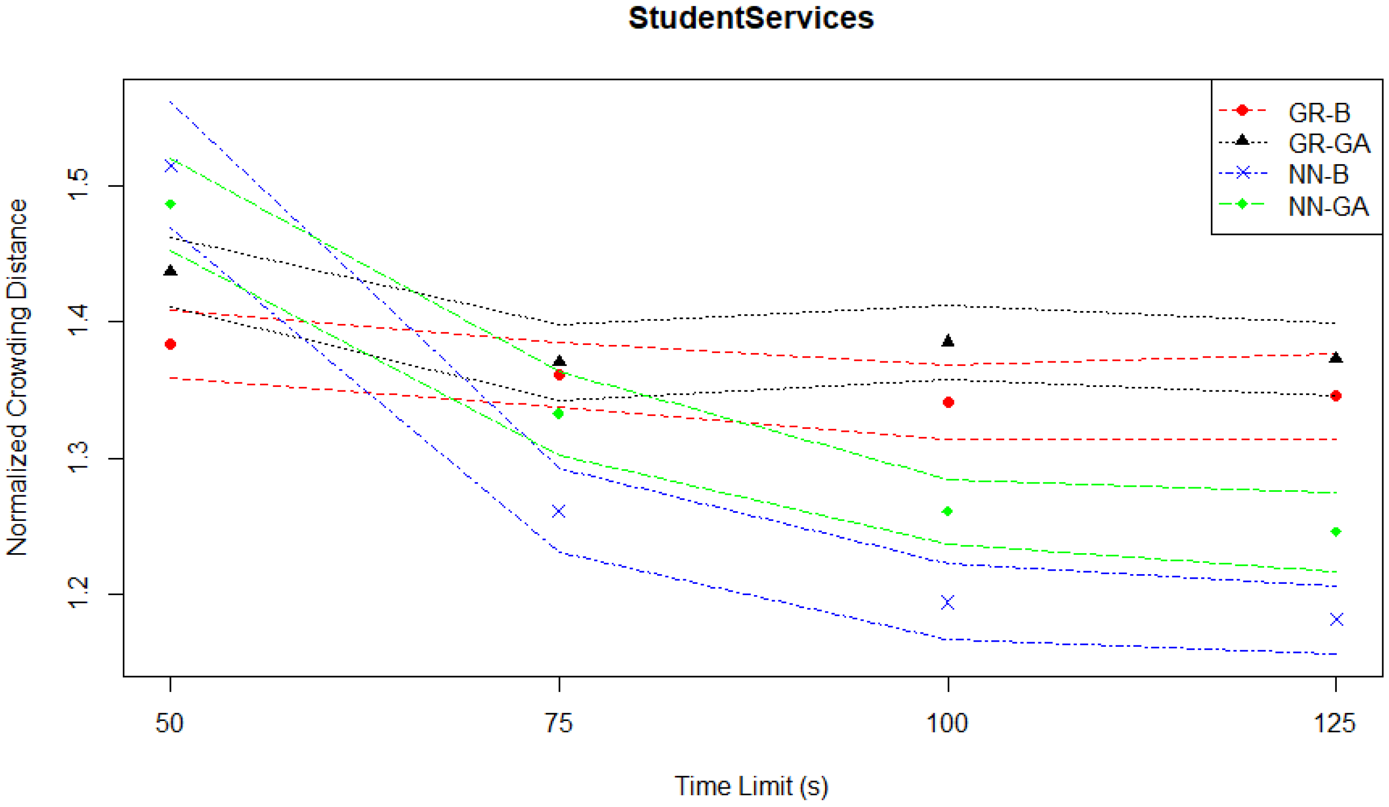
The general pattern of slow improvements in the two Gaussian regression-based pairs, leading to them being out-performed by the neural network-based pairs is also reflected in the normalized Hausdorff distance plot in Figure 5.

The crowding distances depicted in Figure 6 confirm the previously identified patterns of behavior.

4.2. Telecom Simulation Case Study

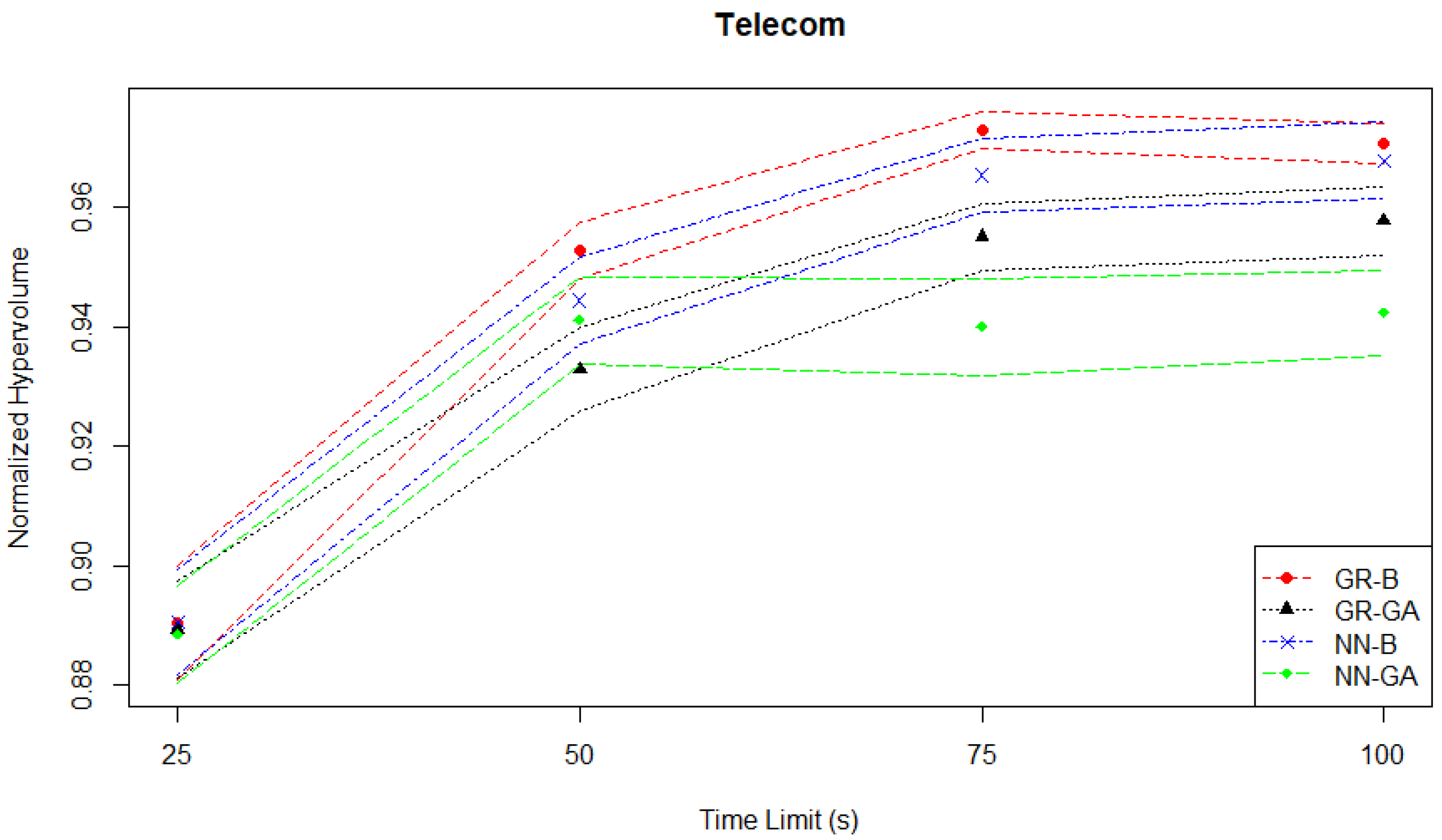
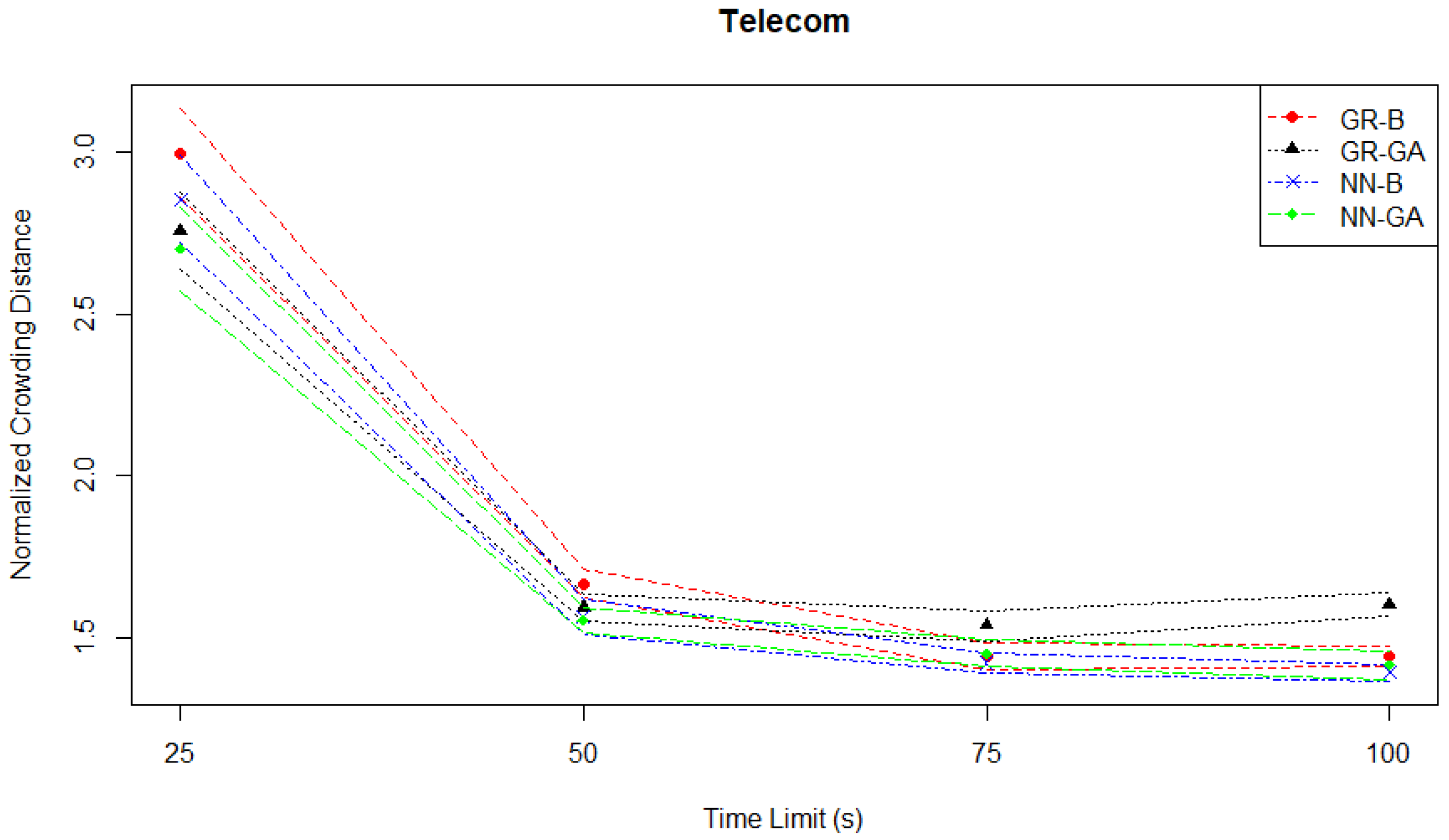
As mentioned in Section 3.1.2, the goal of this case study is to optimize the operations of a telecom company in a competitive market, considering call price, marketing aggressiveness, and revenue components. There is a dramatic improvement in normalized hypervolume initially, as well as a later clear separation of performance between the different MO pairs seen in Figure 7 which depicts the hypervolume evaluation. For example, between the two NN-based pairs (and overall between all four pairs) the NN-GA pair underperforms in terms of not improving from between the time limits of fifty to one hundred seconds, with the second-worst being the GR-GA pair.

Table 2 summarizes the results for the Telecom experiments based on the mean normalized hypervolume performance (${\mu }_{norm}$s) of each MO pair with the best-performing one at each time limit. At a time limit of 25 s, the NN-B pair performs the best among all MO pairs without statistical significance. At the time limits of 50 s, 75 s and 100 s, the “top two MO pairs” in this Telecom case study are different from the Student Services case study, as the GR-B pair outperforms the others. For all these increasing time limits, the NN-B pair delivers a similar performance to GR-B, while the performance differences between GR-B and both GR-GA and NN-GA pairs are statistically significant having p-values less than 0.05. The ${\mu }_{norm}$ produced by GR-B increases from 0.953 to 0.971 as the time limit is doubled.

Table 2. Telecom experiments—normalized hypervolume performance comparison of each MO pair with the best-performing one at each time limit.

Time Limit (s)	MO Pair	${\mathit{\mu }}_{\mathit{norm}}$	$\mathit{\sigma }$	p-Value
25	GR-B	0.890518	4.84 × 10${}^{-3}$	6.22 × 10${}^{-1}$
	GR-GA	0.889344	4.16 × 10${}^{-3}$	9.85 × 10${}^{-1}$
	NN-B	0.890610	4.50 × 10${}^{-3}$	Best
	NN-GA	0.888545	4.13 × 10${}^{-3}$	9.15 × 10${}^{-1}$
50	GR-B	0.952749	2.41 × 10${}^{-3}$	Best
	GR-GA	0.932791	3.53 × 10${}^{-3}$	5.26 × 10${}^{-5}$
	NN-B	0.944377	3.67 × 10${}^{-3}$	1.08 × 10${}^{-1}$
	NN-GA	0.941043	3.70 × 10${}^{-3}$	1.60 × 10${}^{-2}$
75	GR-B	0.972904	1.56 × 10${}^{-3}$	Best
	GR-GA	0.955054	2.82 × 10${}^{-3}$	1.90 × 10${}^{-6}$
	NN-B	0.965317	3.06 × 10${}^{-3}$	6.88 × 10${}^{-2}$
	NN-GA	0.939940	4.08 × 10${}^{-3}$	1.10 × 10${}^{-7}$
100	GR-B	0.970620	1.71 × 10${}^{-3}$	Best
	GR-GA	0.957607	2.92 × 10${}^{-3}$	6.67 × 10${}^{-4}$
	NN-B	0.967764	3.26 × 10${}^{-3}$	7.72 × 10${}^{-1}$
	NN-GA	0.942319	3.62 × 10${}^{-3}$	2.67 × 10${}^{-7}$

Table 2. Telecom experiments—normalized hypervolume performance comparison of each MO pair with the best-performing one at each time limit.

Time Limit (s)	MO Pair	${\mathit{\mu }}_{\mathit{norm}}$	$\mathit{\sigma }$	p-Value
25	GR-B	0.890518	4.84 × 10${}^{-3}$	6.22 × 10${}^{-1}$
	GR-GA	0.889344	4.16 × 10${}^{-3}$	9.85 × 10${}^{-1}$
	NN-B	0.890610	4.50 × 10${}^{-3}$	Best
	NN-GA	0.888545	4.13 × 10${}^{-3}$	9.15 × 10${}^{-1}$
50	GR-B	0.952749	2.41 × 10${}^{-3}$	Best
	GR-GA	0.932791	3.53 × 10${}^{-3}$	5.26 × 10${}^{-5}$
	NN-B	0.944377	3.67 × 10${}^{-3}$	1.08 × 10${}^{-1}$
	NN-GA	0.941043	3.70 × 10${}^{-3}$	1.60 × 10${}^{-2}$
75	GR-B	0.972904	1.56 × 10${}^{-3}$	Best
	GR-GA	0.955054	2.82 × 10${}^{-3}$	1.90 × 10${}^{-6}$
	NN-B	0.965317	3.06 × 10${}^{-3}$	6.88 × 10${}^{-2}$
	NN-GA	0.939940	4.08 × 10${}^{-3}$	1.10 × 10${}^{-7}$
100	GR-B	0.970620	1.71 × 10${}^{-3}$	Best
	GR-GA	0.957607	2.92 × 10${}^{-3}$	6.67 × 10${}^{-4}$
	NN-B	0.967764	3.26 × 10${}^{-3}$	7.72 × 10${}^{-1}$
	NN-GA	0.942319	3.62 × 10${}^{-3}$	2.67 × 10${}^{-7}$

There is a small decrease in $m{u}_{n}orm$ from a time limit of 75 s to 100 s for GR-B. When testing if this difference is statistically significant, the p-value is 0.447, so the decrease is not statistically significant at the 95% confidence level.

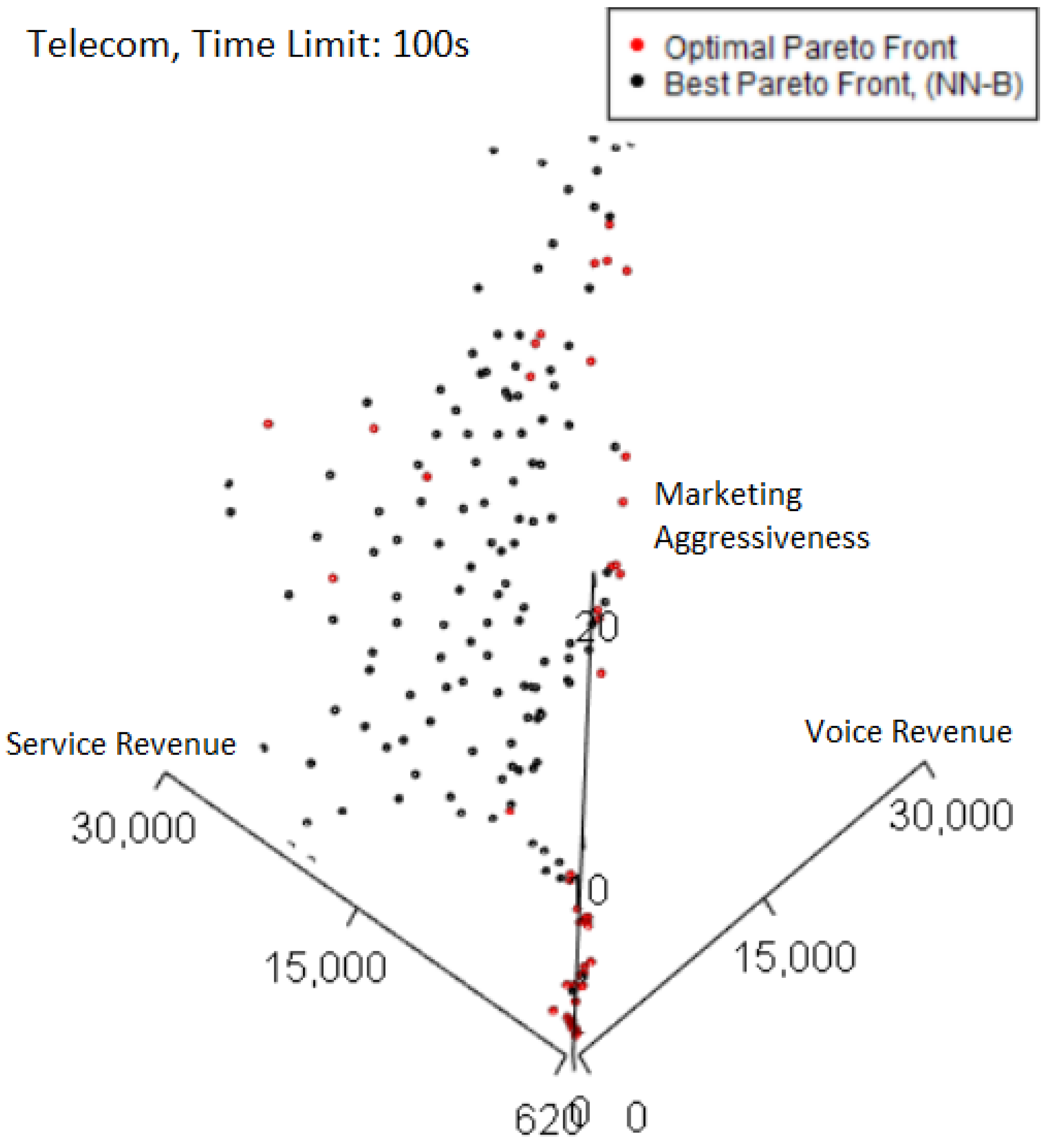
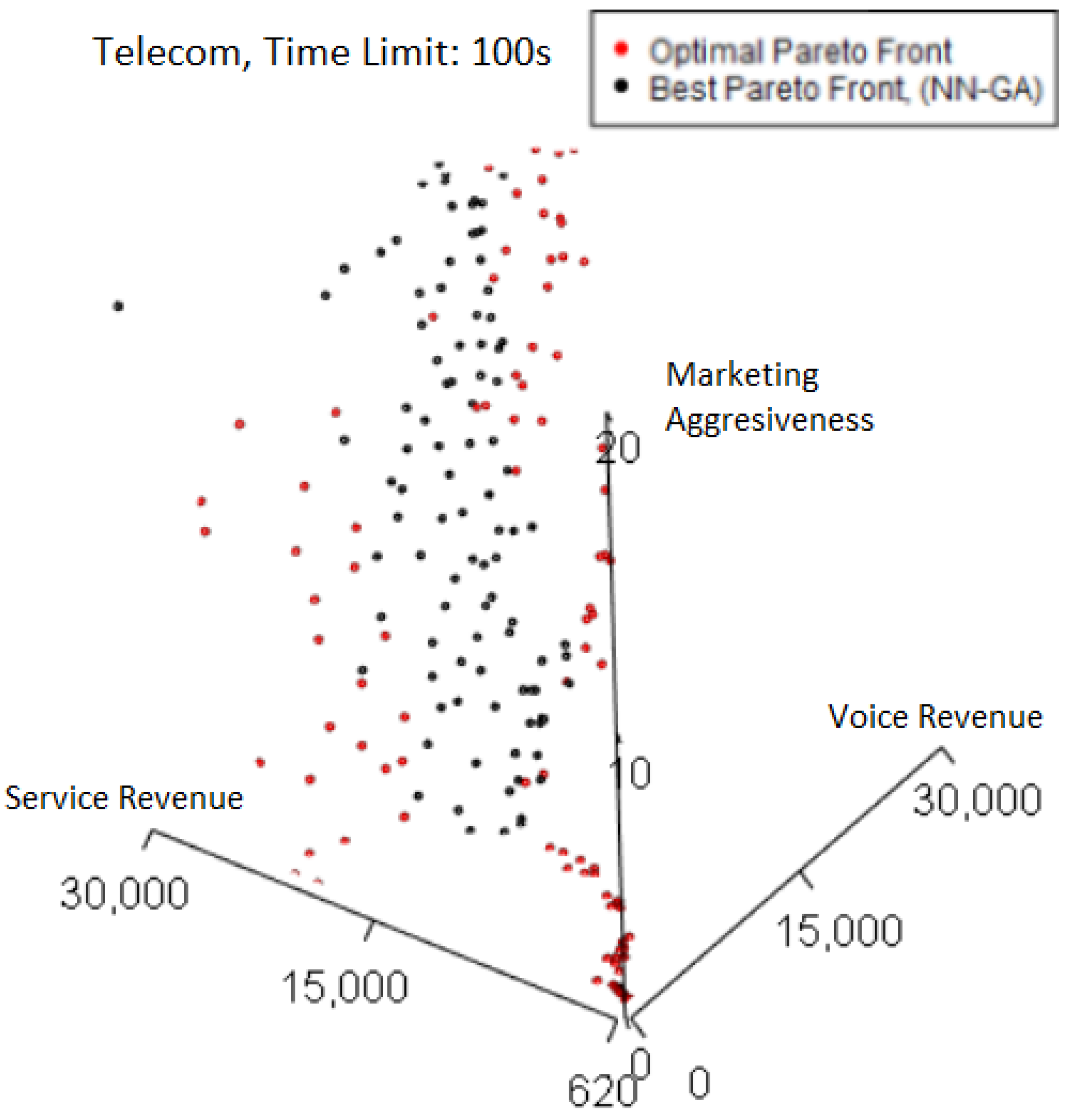
Plotting the best-performing Pareto front from the 100 s case in Figure 8 highlights where losses in quality occur relative to the optimal Pareto front. Where both Pareto fronts overlap, the color is black, corresponding to the best Pareto front. Thus, any red points plotted correspond to points only found on the optimal Pareto front. The right-side edge of the Pareto fronts is where the majority of these points are seen. However, as this best Pareto front has a high normalized hypervolume of 0.997, the quality losses from not including the red points are not major, which implies the Pareto front already captures most of the trade-off solutions by hypervolume.

We can compare the previous situation to the worst-performing 100 s Pareto front (normalized hypervolume of 0.880) plotted in Figure 9. There is a more visually obvious presence of red points on the left and right edges of the worst Pareto front.

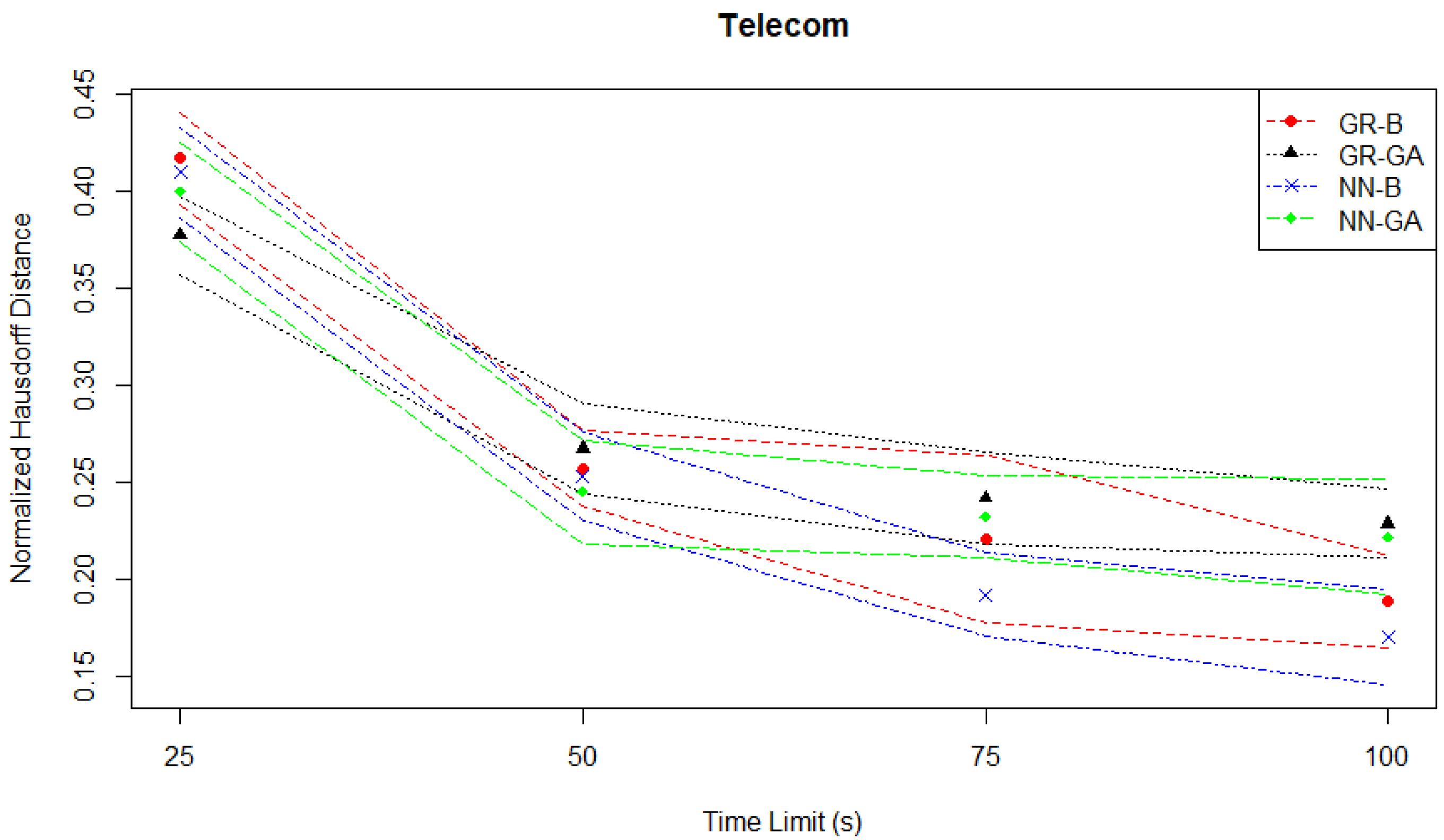
In this case study, the two best-performing MO pairs are the GR-B and NN-B pairs. Thus the main decider of performance is the optimizer rather than the metamodel. This contrasts with the Student Services case where the two best-performing MO pairs are the NN-B and NN-GA pairs which would suggest the main decider of performance is the metamodel rather than the optimizer. If we consider the normalized Hausdorff distances plotted in Figure 10, the two best-performing MO pairs are still the GR-B and NN-B pairs, but the distinctive under-performance of the NN-GA pair relative to the other three MO pairs seen in the hypervolume evaluation at time limits of 75 s or 100 s is not observed in the Hausdorff distance evaluation.

By contrast, when considering the normalized crowding distances plotted in Figure 11, the GR-GA pair has a noticeably higher crowding distance from the other three MO pairs at 75 s and 100 s, although as previously noted it is not the worst-performing in the hypervolume evaluation.

4.3. Continuous News Vendor Simulation Case Study

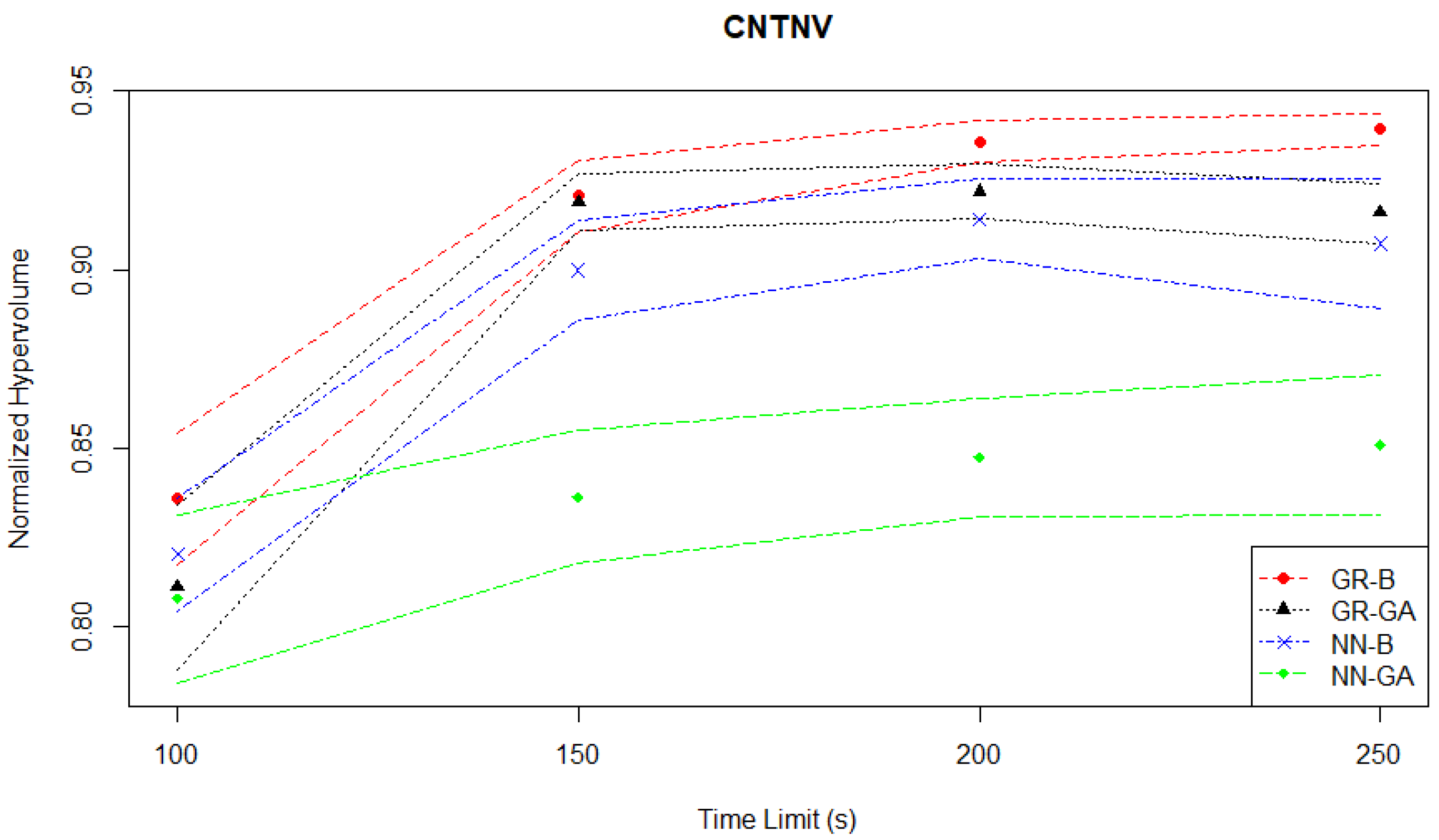
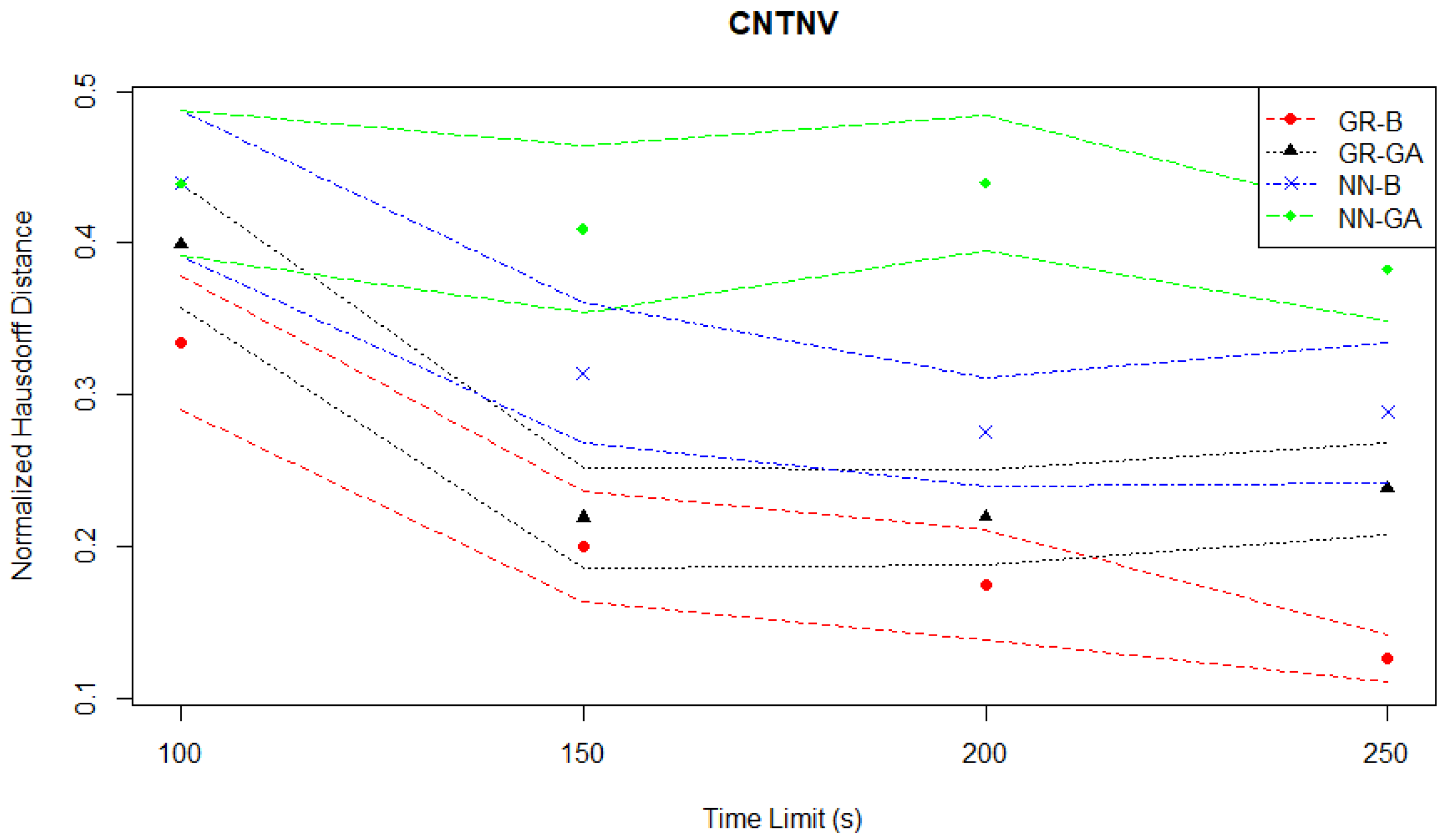
As mentioned in Section 3.1.3, the goal of this case study is to optimize a news vendor’s stock quantity and selling price, considering random daily demand. In both the hypervolume evaluation plotted in Figure 12 and the Hausdorff distance evaluation plotted in Figure 13, the NN-GA pair is a consistent worst-performer when compared to the other three MO pairs.

Table 3 summarises the results from the Continuous News Vendor experiments based on the mean normalized hypervolume performance (${\mu }_{norm}$s) of each MO pair with the best-performing one at each time limit. For any given time limit, the GR-B pair outperforms the rest of the methods. At the 100 s time limit, all methods deliver a similar performance to GR-B, although their ${\mu }_{norm}$s are slightly worse. This observation persists for the time limit of 150 s, while NN-GA performs significantly worse than GR-B. As the time limit increases above 200 s, the performance differences between GR-B and each of the other MO pairs become statistically significant with p-values less than 0.05, and GR-GA ranks the second best-performing method among all. The ${\mu }_{norm}$s of GR-B increases from 0.836 to 0.939 as the time limit increases by a factor of 2.5.

Table 3. Continuous News Vendor experiments—normalized hypervolume performance comparison of each MO pair with the best-performing one at each time limit.

Time Limit (s)	MO Pair	${\mathit{\mu }}_{\mathit{norm}}$	$\mathit{\sigma }$	p-Value
100	GR-B	0.835878	9.33 × 10${}^{-3}$	Best
	GR-GA	0.811036	1.17 × 10${}^{-2}$	1.45 × 10${}^{-1}$
	NN-B	0.820163	8.09 × 10${}^{-3}$	1.32 × 10${}^{-1}$
	NN-GA	0.807869	1.20 × 10${}^{-2}$	7.89 × 10${}^{-2}$
150	GR-B	0.920727	5.03 × 10${}^{-3}$	Best
	GR-GA	0.918869	4.00 × 10${}^{-3}$	4.96 × 10${}^{-1}$
	NN-B	0.899821	7.03 × 10${}^{-3}$	1.18 × 10${}^{-2}$
	NN-GA	0.836305	9.49 × 10${}^{-3}$	7.18 × 10${}^{-8}$
200	GR-B	0.935907	3.00 × 10${}^{-3}$	Best
	GR-GA	0.921874	3.95 × 10${}^{-3}$	9.02 × 10${}^{-3}$
	NN-B	0.914207	5.74 × 10${}^{-3}$	2.30 × 10${}^{-3}$
	NN-GA	0.847465	8.43 × 10${}^{-3}$	2.91 × 10${}^{-9}$
250	GR-B	0.939361	2.22 × 10${}^{-3}$	Best
	GR-GA	0.915885	4.24 × 10${}^{-3}$	9.44 × 10${}^{-5}$
	NN-B	0.907325	9.17 × 10${}^{-3}$	1.21 × 10${}^{-3}$
	NN-GA	0.850925	9.84 × 10${}^{-3}$	8.26 × 10${}^{-9}$

Table 3. Continuous News Vendor experiments—normalized hypervolume performance comparison of each MO pair with the best-performing one at each time limit.

Time Limit (s)	MO Pair	${\mathit{\mu }}_{\mathit{norm}}$	$\mathit{\sigma }$	p-Value
100	GR-B	0.835878	9.33 × 10${}^{-3}$	Best
	GR-GA	0.811036	1.17 × 10${}^{-2}$	1.45 × 10${}^{-1}$
	NN-B	0.820163	8.09 × 10${}^{-3}$	1.32 × 10${}^{-1}$
	NN-GA	0.807869	1.20 × 10${}^{-2}$	7.89 × 10${}^{-2}$
150	GR-B	0.920727	5.03 × 10${}^{-3}$	Best
	GR-GA	0.918869	4.00 × 10${}^{-3}$	4.96 × 10${}^{-1}$
	NN-B	0.899821	7.03 × 10${}^{-3}$	1.18 × 10${}^{-2}$
	NN-GA	0.836305	9.49 × 10${}^{-3}$	7.18 × 10${}^{-8}$
200	GR-B	0.935907	3.00 × 10${}^{-3}$	Best
	GR-GA	0.921874	3.95 × 10${}^{-3}$	9.02 × 10${}^{-3}$
	NN-B	0.914207	5.74 × 10${}^{-3}$	2.30 × 10${}^{-3}$
	NN-GA	0.847465	8.43 × 10${}^{-3}$	2.91 × 10${}^{-9}$
250	GR-B	0.939361	2.22 × 10${}^{-3}$	Best
	GR-GA	0.915885	4.24 × 10${}^{-3}$	9.44 × 10${}^{-5}$
	NN-B	0.907325	9.17 × 10${}^{-3}$	1.21 × 10${}^{-3}$
	NN-GA	0.850925	9.84 × 10${}^{-3}$	8.26 × 10${}^{-9}$

One feature of the Continuous News Vendor optimization problem is that relatively few sets of inputs will correspond to a point on the Pareto front: an exhaustive search encompasses 651 potential input combinations of which only eleven make up the optimal Pareto front. Solution Pareto fronts had between four to fifteen points across all the experiments.

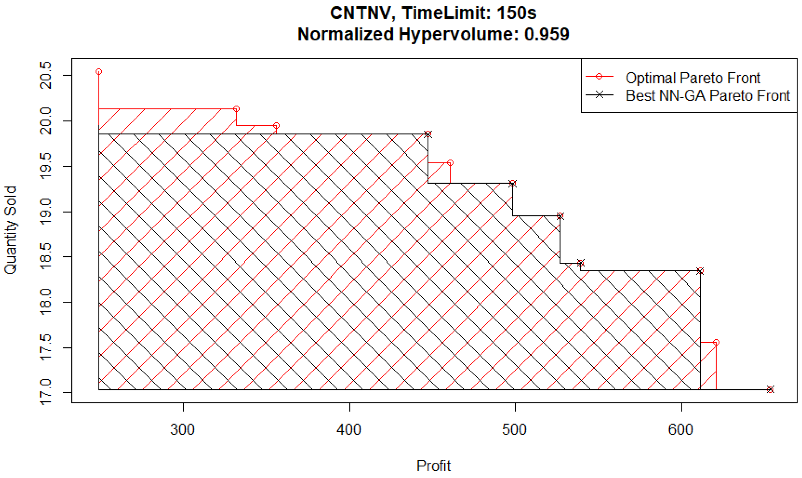
To further analyze the potential effect this causes in solution quality, we consider the Pareto fronts from experiments with a time limit of 150 s. The best-performing Pareto front from a 150 s time limit experiment is plotted in Figure 14 (and is from a GR-GA pair) and can be compared with the best Pareto front from a 150 s time limit experiment specifically from a NN-GA pair, shown plotted in Figure 15. In these figures, the Pareto front of interest and the optimal Pareto front from the FE records are plotted, with the dominated area for each shaded in the appropriate color.

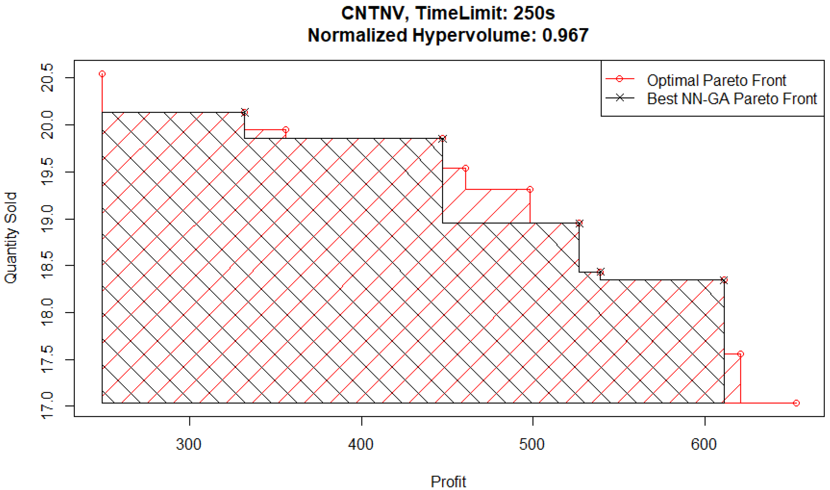
The main area of difference between the two Pareto front solutions is the area corresponding to high quantities sold and low profits. To follow up on this, consider the best NN-GA Pareto front from an experiment with a higher time limit of 250 s plotted in Figure 16. Although the Pareto front from this experiment captures the corner corresponding to high quantities sold and low profits, it does not capture part of the medium quantities sold and medium profits area.

These findings can indicate an issue faced by the genetic algorithm optimizer relative to the Basic optimizer when parent populations are relatively small due to Pareto fronts having only a few points in them. It is harder to identify ex ante which metamodel would under-perform in this situation. However, the hypervolume evaluation shows that the GR-B pair performs the best and the NN-GA pair performs the worst for this problem.

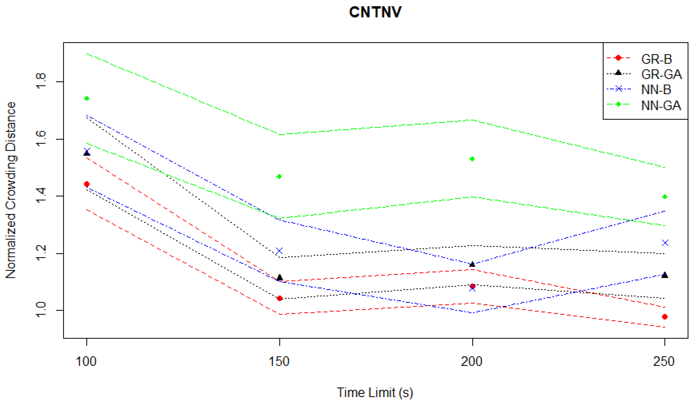
The crowding distance evaluation plotted in Figure 17 confirms that the NN-GA pair has the most widely spaced Pareto fronts of the four pairs, while the GR-B has the closest spacing. Additionally, at a time limit of 250 s, there are GR-B Pareto fronts with normalized crowding distances below 1.

4.4. Dual Sourcing Simulation Case Study

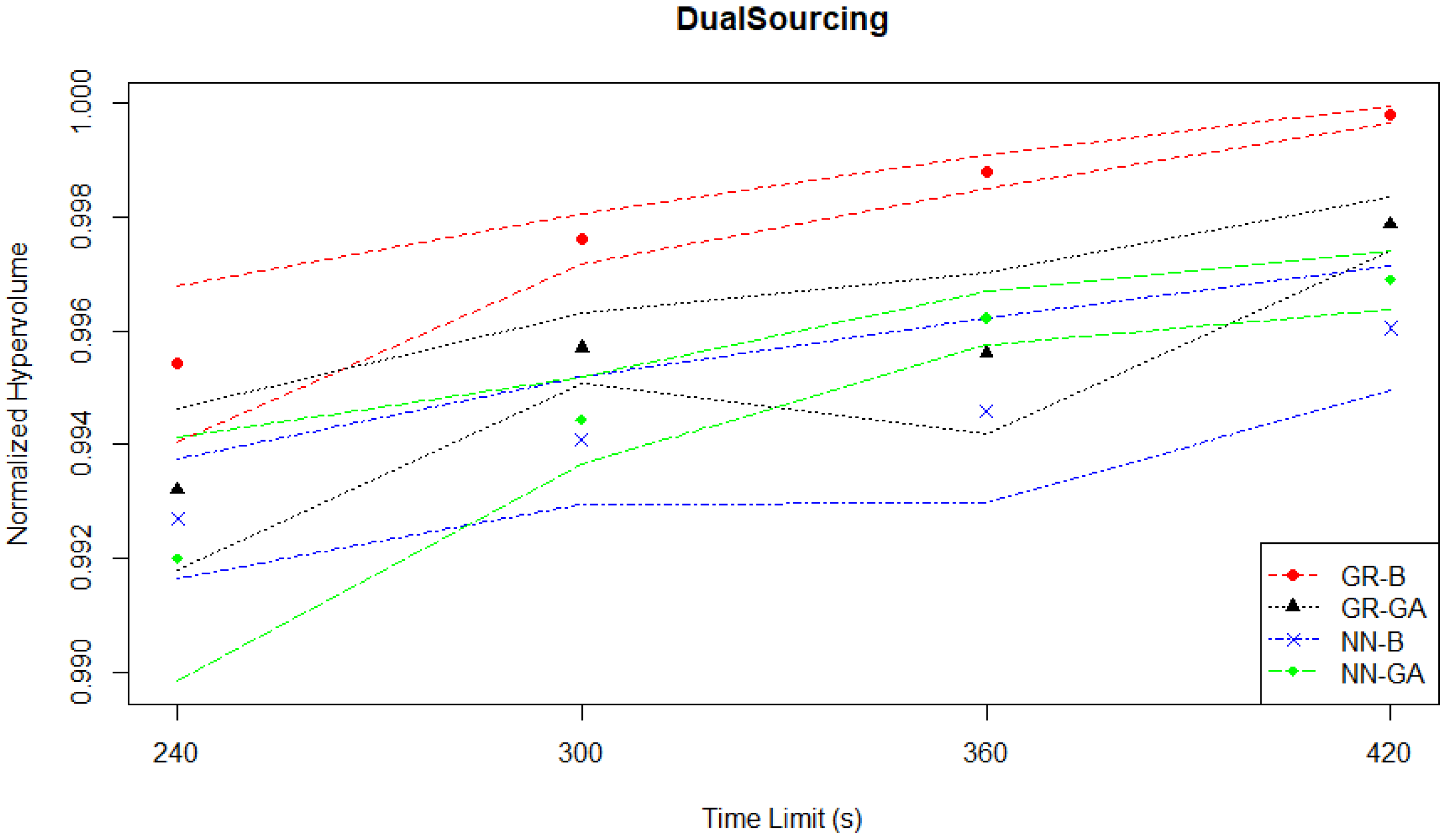
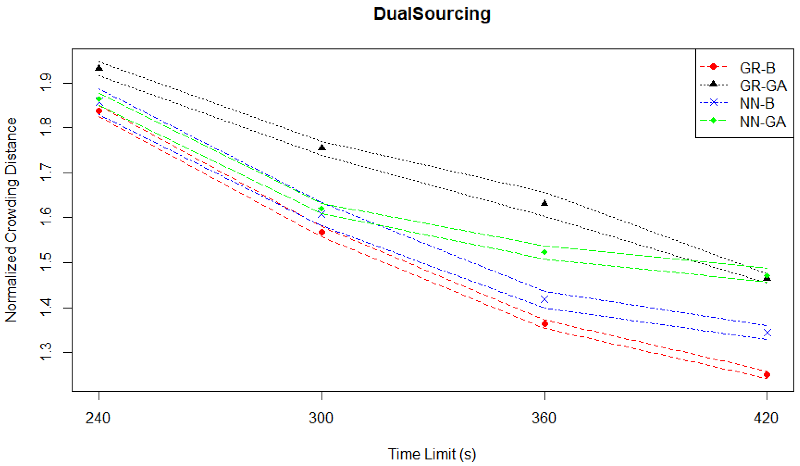
As mentioned in Section 3.1.4, the goal of this case study is to minimize costs and penalties for a manufacturer present in multiple locations, involving procurement from regular or expedited suppliers with varied costs and delays. The Dual Sourcing experiments provide an important contrast with those of the Continuous News Vendor, as the proportion of total input combinations that would be on the Pareto front is much higher (861 of 1681). While solution Pareto fronts have between 383 to 694 points across all experiments, the hypervolume evaluation plot in Figure 18 shows that all MO pairs perform very well, similar to what was observed in the Student Services experiments.

Table 4 summarizes the results from the Dual Sourcing experiments based on the mean normalized hypervolume performance (${\mu }_{norm}$s) of each MO pair with the best-performing one at each time limit. In all time limits (240 s, 300 s, 360 s and 420 s), GR-B outperforms the rest of the MO pairs, and this performance variation is statistically significant with p-values less than 0.05. Regardless of the given time limit, all methods produce a high ${\mu }_{norm}$ over 0.99. The ${\mu }_{norm}$s produced by GR-B increase slightly from 0.9954 to 0.9997 even if the time limit is increased by a factor of 1.75.

Table 4. Dual Sourcing experiments—normalized hypervolume performance comparison of each MO pair with the best-performing one at each time limit.

Time Limit (s)	MO Pair	${\mathit{\mu }}_{\mathit{norm}}$	$\mathit{\sigma }$	p-Value
240	GR-B	0.995415	6.93 × 10${}^{-4}$	Best
	GR-GA	0.993214	7.18 × 10${}^{-4}$	1.10 × 10${}^{-4}$
	NN-B	0.992700	5.32 × 10${}^{-4}$	3.49 × 10${}^{-4}$
	NN-GA	0.991999	1.08 × 10${}^{-3}$	6.89 × 10${}^{-5}$
300	GR-B	0.997616	2.22 × 10${}^{-4}$	Best
	GR-GA	0.995695	3.17 × 10${}^{-4}$	8.17 × 10${}^{-5}$
	NN-B	0.994081	5.68 × 10${}^{-4}$	8.71 × 10${}^{-7}$
	NN-GA	0.994431	3.89 × 10${}^{-4}$	2.18 × 10${}^{-7}$
360	GR-B	0.998792	1.51 × 10${}^{-4}$	Best
	GR-GA	0.995610	7.16 × 10${}^{-4}$	6.25 × 10${}^{-8}$
	NN-B	0.994595	8.22 × 10${}^{-4}$	9.88 × 10${}^{-8}$
	NN-GA	0.996224	2.34 × 10${}^{-4}$	1.82 × 10${}^{-8}$
420	GR-B	0.999778	7.88 × 10${}^{-5}$	Best
	GR-GA	0.997865	2.35 × 10${}^{-4}$	8.83 × 10${}^{-10}$
	NN-B	0.996043	5.52 × 10${}^{-4}$	9.75 × 10${}^{-9}$
	NN-GA	0.996886	2.57 × 10${}^{-4}$	7.44 × 10${}^{-9}$

Table 4. Dual Sourcing experiments—normalized hypervolume performance comparison of each MO pair with the best-performing one at each time limit.

Time Limit (s)	MO Pair	${\mathit{\mu }}_{\mathit{norm}}$	$\mathit{\sigma }$	p-Value
240	GR-B	0.995415	6.93 × 10${}^{-4}$	Best
	GR-GA	0.993214	7.18 × 10${}^{-4}$	1.10 × 10${}^{-4}$
	NN-B	0.992700	5.32 × 10${}^{-4}$	3.49 × 10${}^{-4}$
	NN-GA	0.991999	1.08 × 10${}^{-3}$	6.89 × 10${}^{-5}$
300	GR-B	0.997616	2.22 × 10${}^{-4}$	Best
	GR-GA	0.995695	3.17 × 10${}^{-4}$	8.17 × 10${}^{-5}$
	NN-B	0.994081	5.68 × 10${}^{-4}$	8.71 × 10${}^{-7}$
	NN-GA	0.994431	3.89 × 10${}^{-4}$	2.18 × 10${}^{-7}$
360	GR-B	0.998792	1.51 × 10${}^{-4}$	Best
	GR-GA	0.995610	7.16 × 10${}^{-4}$	6.25 × 10${}^{-8}$
	NN-B	0.994595	8.22 × 10${}^{-4}$	9.88 × 10${}^{-8}$
	NN-GA	0.996224	2.34 × 10${}^{-4}$	1.82 × 10${}^{-8}$
420	GR-B	0.999778	7.88 × 10${}^{-5}$	Best
	GR-GA	0.997865	2.35 × 10${}^{-4}$	8.83 × 10${}^{-10}$
	NN-B	0.996043	5.52 × 10${}^{-4}$	9.75 × 10${}^{-9}$
	NN-GA	0.996886	2.57 × 10${}^{-4}$	7.44 × 10${}^{-9}$

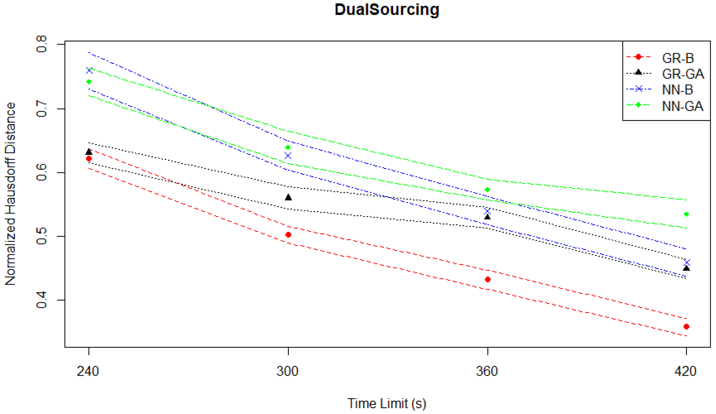
However, the Hausdorff distance evaluation plotted in Figure 19 suggests a large relative separation of solution qualities, which is not observed when considering the normalized hypervolumes. As the Hausdorff distances are normalized, an outlier with a high pre-normalized value will compress the distribution of normalized values towards 0. In fact, the Student Services experiments may exhibit the compression of normalized values issue the most, as the highest plotted point in the Hausdorff distance evaluation plot in Figure 5 which corresponds to the upper confidence interval for NN-GA at the 50 s time limit is close to 0.3, in contrast to the highest plotted point in the Hausdorff distance evaluation for the Dual Sourcing case which is 0.8. The definition of the Hausdorff distance can lead to it being very sensitive to the possibility of a “very bad” solution that is part of a solution Pareto front leading to a very high distance, even though the corresponding point in objective space would not greatly affect the front’s measured hypervolume.

However, the normalized crowding distances plotted in Figure 20 not only support a significant improvement in Pareto front quality in terms of density, but the patterns of relative performance differ between the Hausdorff distance and crowding distance measures. Taken together, these two suggest that a high level of density is not required to properly characterize the Pareto front.

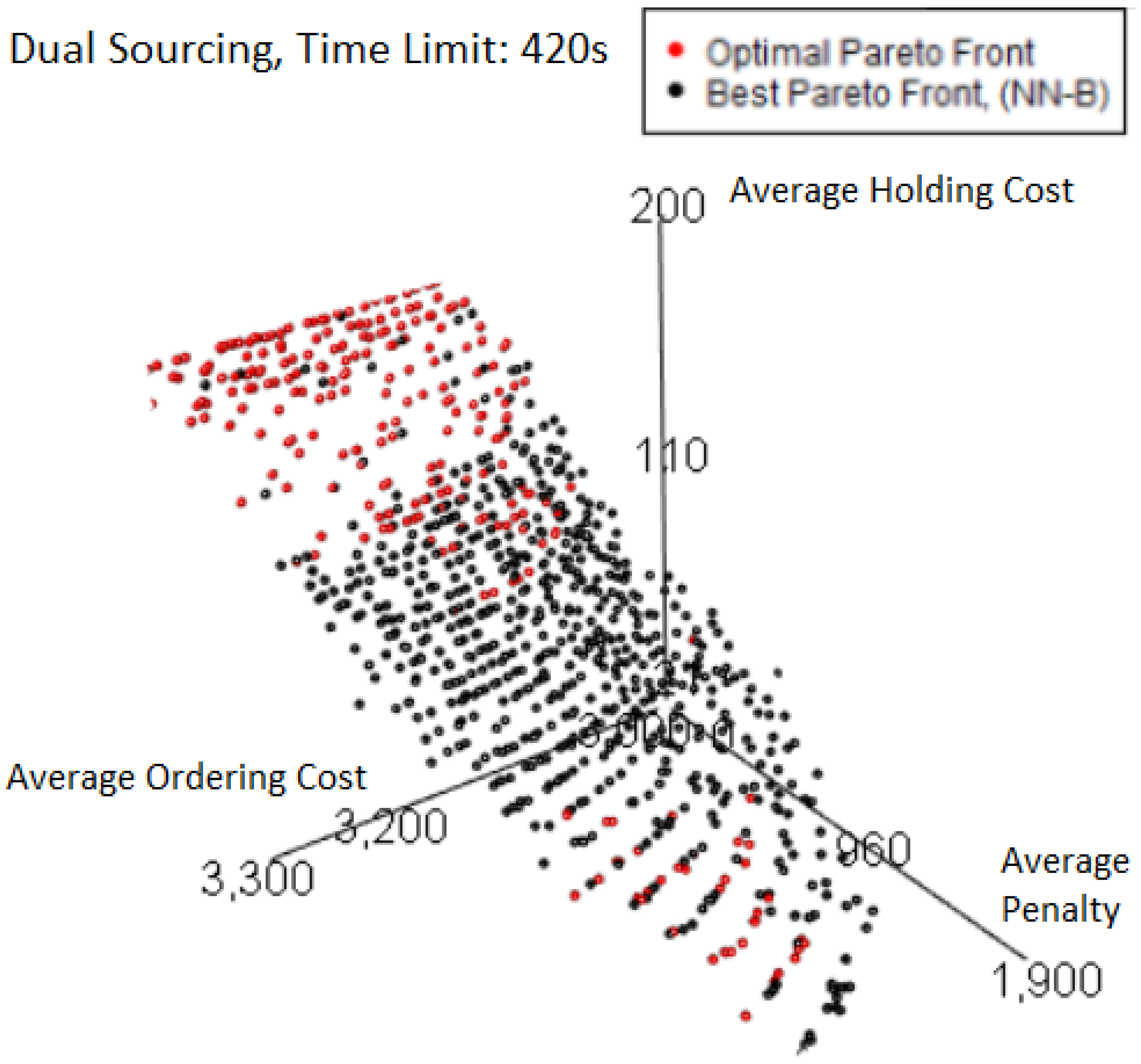
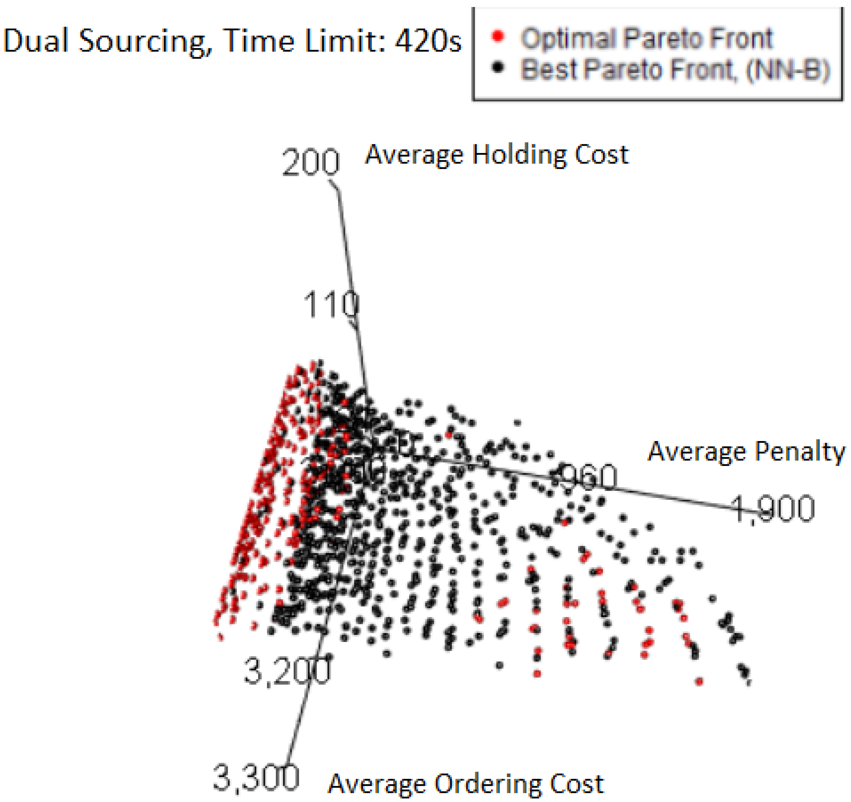
We can further investigate these features by plotting the best Pareto front obtained from a 420 s time limit in Figure 21 which has a normalized hypervolume above 0.999 despite showing a large section of red points that were missed but do not result in significant loss.

Viewing the Pareto front from another angle, as in the plot Figure 22 shows clearly that the large amount of red points seen previously are very close to (many are exactly on) the plane of minimum average penalty. In this case study, it is entirely plausible to have exactly 0 average penalty, as this corresponds to the stock never running out in all the simulation runs done for the FE. There are also a number of points with very small average penalties as well for the same reason. Not only does this follow the general pattern of corners or boundary edges having the majority of “misses” by MO pairs, but in this case, the hypervolume loss is so extremely small because only a couple of points already capture all the relevant space.

4.5. Best-Performing MO Pair

In

Table 5. Best-performing MO pairs per case study.

Case Study	Best MO Pair (s)	${\mathit{n}}_{\mathit{best}}$
Student Services	NN-B & NN-GA	3
Telecom	GR-B & NN-B	3
Continuous News Vendor	GR-B	4
Dual Sourcing	GR-B	4

, we provide the $n_{best}$ value which is the number of times that an MO pair performs the best along with the other top-ranking MO pairs delivering a similar performance to the best (if there are any) considering all four time limits per case study.

The GR-B pair is the best overall option in three of the four case studies with a total $n_{best}$ value of 11. The Basic optimization method (B) is the winner when compared to the genetic algorithm metaheuristic, as this method appears as part of the top-ranking MO pairs in almost all cases.

4.6. Experimental Computational Costs

Table 6. Experimental computational costs.

Simulation	MO Time (min)	FE Time (min)	FE Record Time (min)	FE Record Size (KB)
Student Services	352	672	3.6	13
Telecom	205	557	3.7	21
Continuous News Vendor	462	1541	24.2	13
Dual Sourcing	337	3981	10.7	40

shows the MO Time which is the real-world time taken to run the experiments on each simulation problem. While this does not include the time taken for the associated FEs (as these are looked up from the record) the FE times are recorded and “paid for” with the allowed time limit. As a result, an experiment that is given a time limit of 60 s may run for 15 s of the user time, and end with 15 s of MO time and 45 s of FE time. The “FE Record Time” is the time taken to generate the full list of FEs, and helps demonstrate the savings when many experiments are run. For example, the Student Services experiments took under 6 h, but were able to save an additional 11 h by using the FE records. The gains are largest in the Dual Sourcing case where a higher proportion of the allowed time limit is spent on FEs, such that even though time limits are higher for the Dual Sourcing experiments, the real-world time spent does not increase proportionally.

5. Discussion

In the experimental investigation of four simulation optimization problems, it turned out that two of them (Student Services and Dual Sourcing) can be considered straightforward in that all the MO pairs evaluated performed similarly and produced high-quality Pareto fronts. In the other two (Telecom and Continuous News Vendor), there was more of a separation of quality with different patterns between the MO pairs evaluated, which comes from the way in which the metamodels estimate objective values for the inputs being explored by the optimizers. One can form more intuitive relationships from MO pair performance patterns to response surface properties than starting from the simulation components or domains, as there are only a limited number of MO pair performance patterns.

Ideally, even a problem with a computationally intensive simulation model of interest would have well-behaved response surfaces, allowing a metamodel to identify areas of interest quickly and with confidence. This would enable the use of expensive FEs more sparingly, focusing on those areas of interest identified by the metamodel to maximize the precision of the optimization. However, being “well-behaved” is not necessarily a simple property that would hold for all MO pairs that might be employed. As seen, some MO pairs may perform better than others for certain problems of interest. Additionally, multi-domain problems may or may not behave similarly to the problems of any particular component domain [40].

The application of metamodeling to ABS is currently a topic of great interest and ongoing research. In the Student Services case study, we showed that despite the agent-based behavior of the model, it was still able to be solved to a high standard across all evaluated MO pairs. In fact, for this problem, the agents’ decision-making did not lead to a complex response surface. In contrast, a more challenging problem like the one investigated in the Continuous News Vendor case study has a simple simulation model but a response surface that is not equally responsive to different MO pairs.

It is important to note that the FE times are based on a fixed record. However, the time limit stopping condition treats a second of FE time as equivalent to a second of metamodel or optimizer time. Therefore, if one runs experiments on problems where records were generated on a slower system, the faster system will always obtain better quality solutions within the same time limit, as the faster system has more computational resources. It will be possible to replicate previous results by creating a different version of the record with scaled decreased FE times. This will better match what the faster system is experiencing. Additionally, a smaller time limit can be used in the same proportion. This approach still allows the user to use records, but avoids having to set up numerous simulation models.

While handy for experimental work like that detailed here, the downside of using an FE recording approach is that it does introduce an issue if there is a desire to create records for simulation models with a large input space due to memory constraints. Furthermore, referencing the records will take longer as they grow in size. This can lead to a memory-computation cost tradeoff. However, for the simulation models presented in this paper, the records are small enough so that they do not require a lot of memory to load. The ability to use records without having to run the underlying simulation model is also a form of experiment enabler, especially if the associated model would otherwise be simply inaccessible.

6. Conclusions

In this paper, we have presented and tested a comprehensive methodology designed to facilitate the systematic application and evaluation of metamodeling and optimization heuristics in the form of MO pairs. Our methodology enables researchers to compare setups experimentally, in a way that allows drawing general conclusions about the optimal MO pairs. Hence, the aim detailed in Section 1.4 has been fulfilled. The methodology has been tested with the help of a test environment that allows algorithmic testing and evaluation of MO pair performance for different types of problems. We have demonstrated its use with the help of four illustrative case studies. The performance of the different four MO pairings we tested suggests that patterns of relative performance (and thus the ideal choice) may differ between different models that they are asked to solve.

By critically assessing our work, we have identified several limitations that will need further research: (1) Our methodology has not been tested on highly complex models. (2) Our test cases are limited to the OR domain. (3) Instead of conducting experiments with different time limits, it may be more efficient to run experiments up to the highest time limit and use vertical slicing to directly investigate the evolution of Pareto front quality over time. (4) To evaluate Pareto front quality, we can incorporate additional metrics from the multiple objective literature to gain further insights into the performance of MO pairs. (5) The field of metamodeling and optimization offers numerous other metamodels and optimizers that have not yet been tested.

This presents several opportunities for future work. The most straightforward would be to increase the number of simulation models, metamodels and optimizers available for experimentation and performance comparisons. Since simulation models are represented in the environment by records of their input-objective outcomes (including time taken), additional simulation models from other domains and implemented in various simulation platforms can be integrated into the environment and made accessible for comparison purposes. Better domain coverage from this can enable testing of generalizability across a number of domains and problems without having to manage data links to external simulators for each one.

Additionally, where there are parameters for these components that are currently treated as fixed across all uses in these case studies, it may be possible to improve a component by augmenting them with algorithmic hyper-parameter optimization, although this is a non-trivial addition when keeping to the design goal of allowing generalizability to future models. The possibility exists that having a larger variety of less individually optimized metamodel or optimizer options is more efficient in terms of component-possibility coverage.

Another important aspect that requires further investigation is the question of when and why simulation models behave similarly in terms of the performance of MO pairs. While models with similar response surface properties will show similar patterns of MO pair performance, the question remains of identifying the more abstract properties that lead to these similarities in the performance of MO pairs. Alternatively, the possibility of building a selection-type hyperheuristic that explores the space of metamodel and optimizer selection within the optimization process and selects an optimal pair on the fly could potentially be more beneficial for practical applications. This approach could also be generalizable if performance patterns can be detected early enough in the optimization process to justify allocating computational resources to the hyperheuristic layer, rather than a simple initial MO pair selection.