1. Introduction
The emergence and development of Artificial Intelligence in various key domains has intrinsic ties with games. The earliest AI program was a draughts game written by Christopher Strachey in 1951. It successfully ran for the first time on the Ferranti Mark I universal electronic computer at the University of Manchester in the UK. Impressed and influenced by Strachey and Turing, Arthur Samuel took on the draughts project’s key points initiated by Strachey in 1952 and expanded it considerably over the years, allowing the program to learn from experience. As one of the earliest cases of Artificial Intelligence search technology, these advancements enabled the program to win a match against a former draughts champion from Connecticut, USA. Samuel’s experiments and accumulation in the game technology field helped him propose the concept of machine learning in 1959.
In March 2016, Google’s Deep Mind developed the Alpha Go system, defeating the then human world champion of Go, Lee Sedol, thus creating a global sensation. The Go board is composed of 19 horizontal lines and 19 vertical lines, with a total of 19 × 19 = 361 intersections. Each intersection on the Go board has three possibilities: a black stone, a white stone, or empty. Therefore, Go has a staggering number of possible positions: 3 to the power of 361. Each turn in Go has 250 possibilities, and a game can last up to 150 turns. As a result, the computational complexity of Go is 250 to the power of 150, which is approximately 10 to the power of 170. However, the observable number of atoms in the entire universe is only 10 to the power of 80. This clearly demonstrates the complexity and variability of the game of Go. In principle, AlphaGo uses a modified version of the Monte Carlo algorithm, but more importantly, it enhances its learning effect by leveraging deep reinforcement learning [
1].
Reinforcement learning is a machine learning method that utilizes sequence information consisting of actions from agents, states from the environment, and rewards through interaction between agents and the environment [
2]. The Q function is a fundamental concept in reinforcement learning, which can output the value of action a in state s. Learning an accurate Q function can help policy functions update in the correct direction. Due to the influence of updated formulas, inflexible function estimation methods, and noise, the Q function often has bias in estimating the true Q value [
3,
4]. The deviation in Q-value estimation may lead to the algorithm converging to a suboptimal policy, resulting in a decrease in algorithm performance.
Bright possibilities also exist for the application of deep reinforcement learning in multi-agent systems like drone formation control, cooperative-control multi-robots, and traffic vehicle control, all of which can significantly improve collective gains and enhance the quality of human life. Multi-agent reinforcement learning can be seen as the expansion of single-agent reinforcement learning algorithms in a multi-agent scenario. The migration of policy gradient algorithms based on Q-function learning to multi-agent scenarios will bring more severe impact due to the bias in Q-function estimation. The bias in the estimation of the Q-function will increase the variance of the network gradient and affect the update process of the policy network. In a multi-agent environment, with the increase in agents, the difficulty of updating the policy network in the correct direction increases exponentially, so such a bias will bring greater difficulties to policy learning in multi-agent scenarios.
This article primarily revolves around the research of the Q-value estimation bias problem in Multi-Agent Deep Reinforcement Learning, and constructs a new multi-agent experimental environment. The detailed research objectives are as follows:
1. The method of combining multiple Q networks to reduce the Q-value estimation bias is further studied, according to the feature of all agents having the same structured Q network in the architecture of centralized training with distributed execution in multi-agent systems. In this research objective, we aim not to increase the network parameters of the model, but to alleviate the problem of Q-value underestimation caused by dual Q networks by organizing multi-agent systems.
2. The method of using softmax operation to reduce Q-value estimation bias is further studied, and the softmax operation method is applied to multi-agent algorithms. This research aims to utilize the characteristics of softmax to reduce the overestimation bias of Q-value, and to simplify the action space used for computation in multi-agent systems, thereby reducing computational load.
3. For scientific research on multi-agent reinforcement learning, we have developed the multi-agent tank environment of the University of Electronic Science and Technology of China (UESTC-tank). This is a tank simulation game environment with multiple units and scenes, which can generate cooperative, adversarial, and mixed task scenarios. It can achieve competitions of player vs. player, player vs. AI, AI vs. AI types, and collect battle data for model training. It can support unit editing, map editing, and rule editing, and has good scalability. We tested our proposed algorithm on UESTC-tank and achieved good experimental results.
The rest of this paper is arranged as follows: Firstly, we introduced the research context in
Section 2. Then, in
Section 3 and
Section 4, we introduced the multi-agent twin-delayed deep deterministic policy gradient and multi-agent soft-maximization twin-delayed deep deterministic policy gradient algorithms. In
Section 5 and
Section 6, we introduced the multi-agent particle environment and multi-agent tank environment, conducted experiments, and analyzed the results. After summarizing our work so far,
Section 7 provides limitations and conclusions of the paper.
2. Research Background
2.1. Deep Reinforcement Learning
Reinforcement learning can be modeled as an agent is faced with a sequential decision making problem. At time t, the agent observes state from the environment, and adopts action based on its policy. Due to the interaction of the agent, the environment transitions from state to the next state and returns a reward r to the agent. If the environment transitions to a termination state, we call it the end of an episode. The goal of reinforcement learning is to enable agents to learn an optimal policy to obtain the maximum cumulative reward (called return) from the entire episode.
Reinforcement learning algorithms can be classified into policy function-based [
5] and value function-based [
6]. A common value function is the action value function, also known as the Q function, which inputs the current state of the environment and the action taken by the agent, and outputs an estimate of the expected return for that state–action pair. When the agent learns the optimal Q function, the optimal policy can be to select the action that can maximize the output value of the optimal Q-function in any state. In deep reinforcement learning, we use deep neural networks to fit the policy function, value function, and Q function, hence also known as policy networks, value networks, and Q networks.
2.2. Deep Q-Learning Algorithms
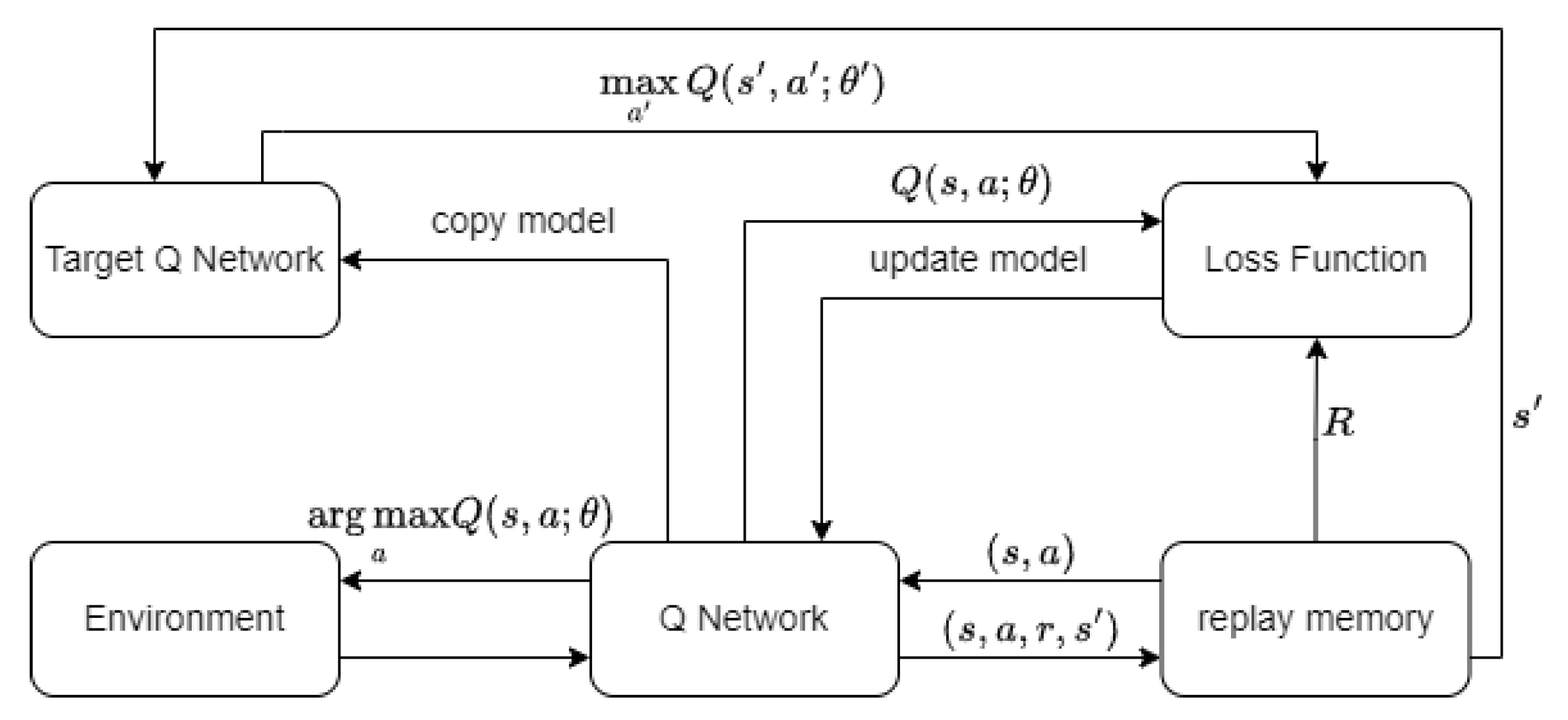
Mnih and others [
6] were the first to integrate deep learning and traditional reinforcement learning algorithm, thus proposing the DQN algorithm. This pioneering piece of work marked the first end-to-end deep reinforcement learning algorithm using only Atari game pixel data and game scores for reinforcement learning state information. Finally, the trained network could output action-value functions or Q-values for each action. From this, the decision with the highest corresponding Q-value is selected. The entire structure of the DQN algorithm is shown in
Figure 1.
The DQN algorithm introduces the experience replay mechanism, which stores the sample tuple of the agent at each time step into an experience replay pool. During reinforcement learning training, a batch of samples is sampled from the experience replay pool and the neural network is updated using gradient descent. The use of experience replay mechanism greatly improves the data utilization of reinforcement learning algorithms and to some extent reduces the correlation between training data and sequences.
Another important contribution of the DQN algorithm is the concept of the target network, which achieves stable value estimation. The target value
y for updating the Q network by computing the loss function is represented as:
where
represents the target network.
is a discount factor (0 <
< 1), used to give a preference for rewards reaped sooner in time.
is the action that allows the Q function to take the maximum value. The structure of the target network is the same as the Q network, but its parameters are only copied from the Q network every certain number of iterations.
The Q network updates its parameters in each round by minimizing the loss function defined in Equation (
2):
E represents mathematical expectation, which is calculated using Monte Carlo estimation method in practice, taking the average value of batch samples to estimate. The neural network is updated to make the Q network approximate the target value y, which essentially applies the Bellman equation. The use of target network helps improve the stability of the algorithm, and experiments have shown that NPC controlled by DQN algorithm can reach the level of professional players in many Atari games.
The DDPG [
7] algorithm can be seen as a combination of Deterministic Policy Gradient (DPG) algorithm and deep neural networks, and it can also be seen as an extension of DQN algorithm in a continuous action space. It can solve the problem of the DQN algorithm’s inability to directly apply to continuous action space, but there is still the problem of overestimation of Q values. The DDPG algorithm simultaneously establishes a Q network (critic) and a policy network (actor) [
8]. The Q network is the same as the DQN algorithm, updated using a temporal difference method. The policy network utilizes the estimation of the Q network and is updated using policy gradient method.
In the deep deterministic policy gradient algorithm, the policy network is a deterministic policy function represented as , with the learning parameters represented as . Each action is directly computed by , without sampling from a random policy.
2.3. Estimation Bias of Q-Learning Algorithms
When an agent executes action
a in state
s, the environment will transition to state
and return an immediate reward
r. In the standard deep Q-learning algorithm, we update the Q-function using Equation (
1). When using neural networks and other tools as function approximators to handle complex problems, there can be errors in the estimation of Q values, which means:
where
is a zero-mean noise term,
is a Q function that can output the real Q value, or the optimal Q function.
However, when using the maximum operation to select actions, there can be errors between the estimated Q values and the real Q values. The error is represented as
:
Considering the noise term , some Q values may be underestimated, while others may be overestimated. The maximization operation always selects the maximum Q value for each state, which makes the algorithm overly sensitive to the high estimated Q values of the corresponding actions. In this case, the noise term causes , resulting in the problem of overestimation of Q values.
The TD3 [
9] algorithm introduces clipped Double Q-Learning on the basis of the DDPG algorithm, by establishing two Q networks
to estimate the value of the next state, and using the minimum estimated Q-value of two target networks to calculate the Bellman equation:
where
y is the update target for
and
, and
is the policy network.
Using clipped Double Q-Learning, the value estimation of target networks will not bring excessive estimation errors to the Q-Learning target. However, this update rule may cause underestimation. Unlike actions with overestimated Q values, actions with underestimated Q values will not be explicitly updated.
Here is proof of the underestimation of the clipped Double Q-Learning, the two outputs values (
and
) of the Q network, and that
is the real Q value. The errors brought by the fitting of the two networks can be defined as:
Assuming errors
and
are two independent random variables with nontrivial zero-mean distributions, the minimization operation of the TD3 algorithm introduces an error. The error denoted as
D is as follows:
where
r is the reward and
is the discount factor. Let
Z be minimum value between
,
, and we have:
Obviously, there is , and . Therefore, we can deduce that , which means that the clipped Double Q-Learning usually has underestimation.
Specifically, in order to have a more intuitive perception of underestimation, we can assume that the error follows an independent and uniform distribution in the range
. Since the estimated Q values and the true Q values have error
that follows a uniform distribution, the probability density function and the probability distribution are represented by
and
, respectively:
Also, since
and
are independent, it follows that:
Let
Z be the minimum value between
,
. The probability density function and cumulative distribution function of
Z are represented as
and
, respectively:
Therefore, the expected value of
Z can be calculated as follows:
Thus, it has been theoretically proven that the Q network update in the TD3 algorithm will result in an underestimation error for the true Q values.
2.4. Multi-Agent Twin Delayed Deep Deterministic Policy Gradient (Matd3)
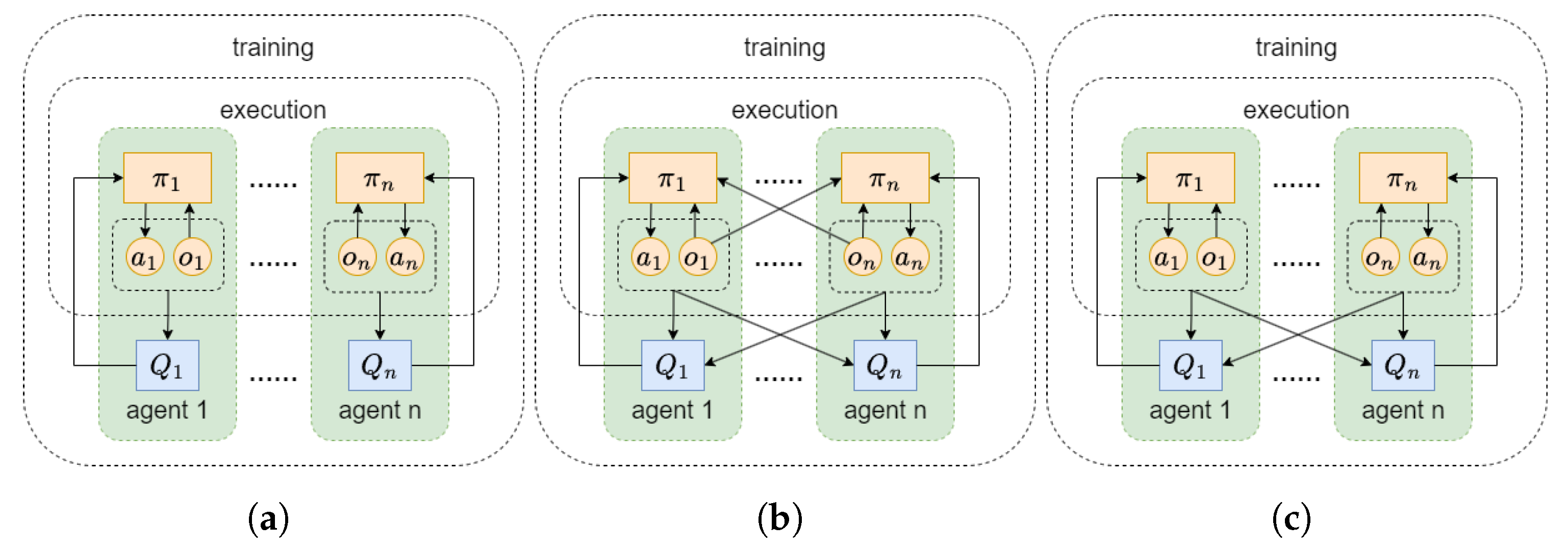
The training modes of multi-agent deep reinforcement learning include Decentralized Training Decentralized Execution (DTDE), Centralized Training Centralized Execution (CTCE), and Centralized Training Decentralized Execution (CTDE), as shown in
Figure 2.
The MATD3 [
10] algorithm extends the single-agent TD3 algorithm to a multi-agent environment, adopting the centralized training decentralized execution reinforcement learning framework. During the behavior execution process of the agents, each agent inputs their local observation information into the policy network, outputs deterministic actions, and during the training process, the agents can obtain additional information from other agents to evaluate their own actions.
The problem of Q network estimation bias will have a more severe impact when transferring policy gradient algorithms with Q-functions to a multi-agent scene, because the estimation bias of the Q network can increase the variance of the neural network gradient and affect the update process of the policy network neural network. In a multi-agent environment, as the number of agents increases, the difficulty of updating the policy function in the correct direction increases exponentially. The MATD3 algorithm simply extends the TD3 algorithm to a multi-agent environment, and there are still problems with the underestimation of Q values. In a multi-agent environment, this bias will have a greater impact on the agent’s strategy learning.
3. Multi-Agent Mutual Twin Delayed Deep Deterministic Policy Gradient (M2ATD3)
In multi-agent scenarios, single Q network algorithms such as Multi-Agent Deep Deterministic Policy Gradient (MADDPG) have problems of overestimation. However, twin Q network’s MATD3 algorithm, while resolving the overestimation of Q value, inevitably leads to underestimation. The Multi-Agent Three Delayed Deep Deterministic Policy Gradient (MATHD3) algorithm is proposed to create a third Q network. The overestimated results from it, and the underestimated results from the minimization of the first two Q networks, are added together by adjusting the weight hyperparameter
, and an unbiased estimate of the actual Q value can be obtained. In multi-agent algorithms, we denote the observation received at runtime by agent i as
, and the full state information as
, from which the observations
are derived. The Q network update target
of the MATHD3 algorithm is as follows:
where
is obtained by adding noise
to the output of the target policy network
of agent i based on its observation
, that is:
.
While the MATHD3 algorithm effectively reduces bias in Q value estimates, it requires introducing a new Q network, leading to an increase in model parameters and increased model training difficulty.
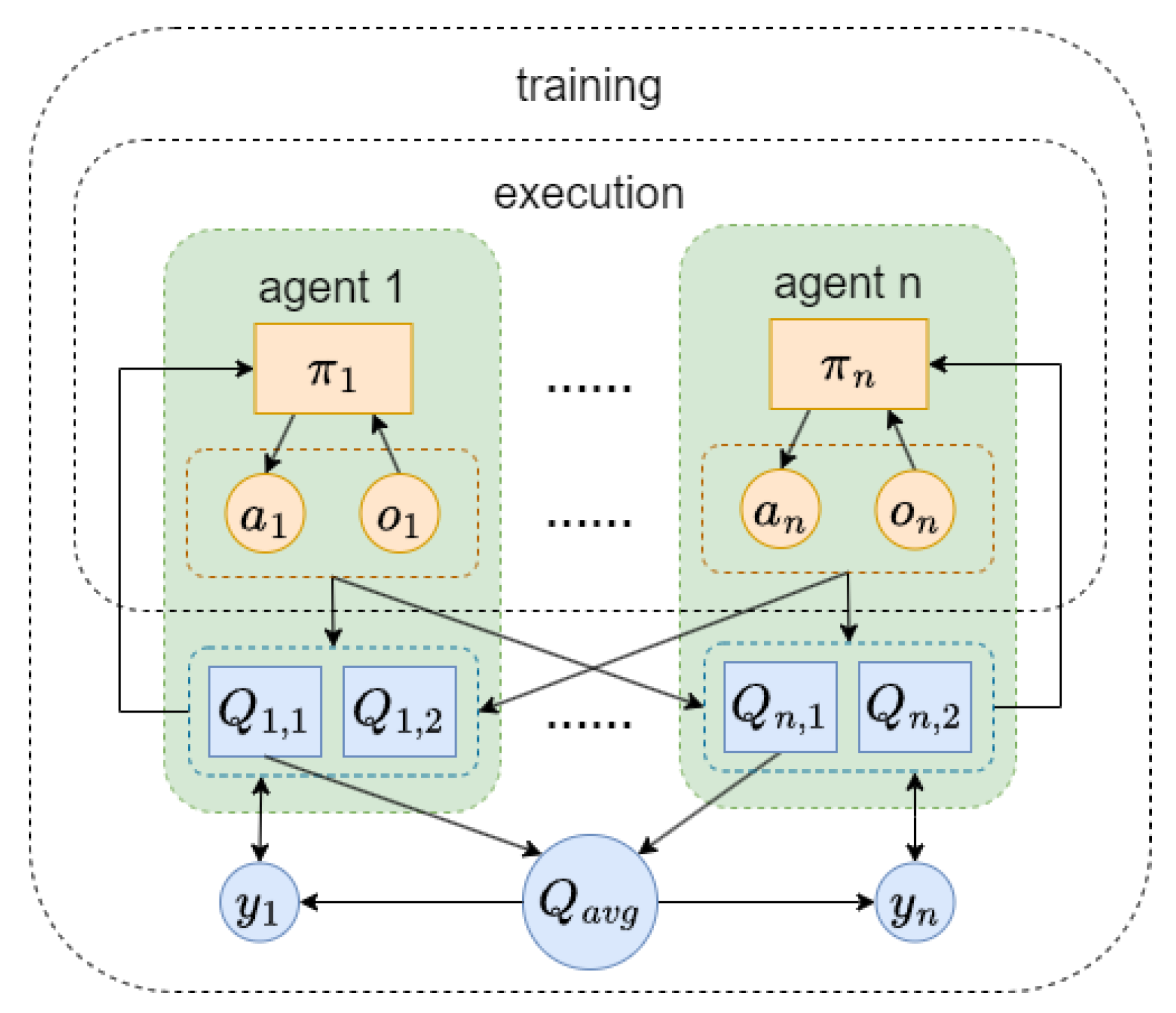
Psychological studies show that humans exhibit overconfidence, typically estimating themselves beyond their actual abilities [
11]. Introducing external evaluations can mitigate this phenomenon. Weinstein suggests that people are unrealistically optimistic because they focus on factors that improve their own chances of achieving desirable outcomes and fail to realize that others may have just as many factors in their favor [
12]. Inspired by this, we propose the Multi-Agent Mutual Twin Delayed Deep Deterministic Policy Gradient (M2ATD3) algorithm. The training mode of M2ATD3 algorithm is shown in
Figure 3.
Single Q networks, affected by noise, always overestimate Q values. Averaging the estimated Q values from each agent’s Q network results in a slightly overestimated mutual Q value estimate. The mutual estimate of the Q value and the minimum value of two Q network estimates for agent i are weighted together to obtain the Q network update target
of the M2ATD3 algorithm:
The mutual estimate of the Q value is overestimated, and the minimization of the twin Q network will lead to underestimation. By adjusting the weight hyperparameter
, in theory, an unbiased estimate of the true Q value of agent i can be obtained. The M2ATD3 algorithm reduces the Q value estimation bias without needing to introduce a new Q network. Moreover, the operation of taking the average of Q value estimates can also reduce the variance of Q value estimate errors [
13], making the training process more stable.
We have maintained the delayed policy updates used in the TD3 algorithm. The TD3 algorithm proposes that the policy network should be updated at a lower frequency than the value network, to first minimize error before introducing a policy update. This method requires updating the policy and target networks only after a fixed number of updates d to the critic.
The M2ATD3 algorithm pseudo code can be found in Algorithm 1.
| Algorithm 1 Multi-Agent Mutual Twin Delayed Deep Deterministic policy gradient |
initialize Replay buffer D and network parameters for t = 1 to T do Select action Execute action and get reward , transition to next state Store the state transition tuple into D for agent i = 1 to N do A sample batch of size S is sampled from D Minimize the loss of two Q-functions, j = 1,2: if t mod d = 0 (d is the policy delay update parameter) then update : Update target network: where is the proportion of target network soft updates end if end for end for
|
5. The Multi-Agent Particle Environment Experiment
The multi-agent particle environment was used as the experimental environment in this study, proposed by Lowe et al. [
17], and used for the verification of MADDPG algorithm. The multi-agent particle environment is a recognized multi-agent reinforcement learning environment [
10,
14,
17], including different tasks, covering competition, cooperation, and communication scenarios in multi-agent problems. The particle environment is composed of a two-dimensional continuous state space, in which agents move to fulfill specific tasks. The state information includes the agent’s coordinates, direction, speed, etc. The shape of the agent is spherical, and actual collision between agents is simulated through rigid body collision.
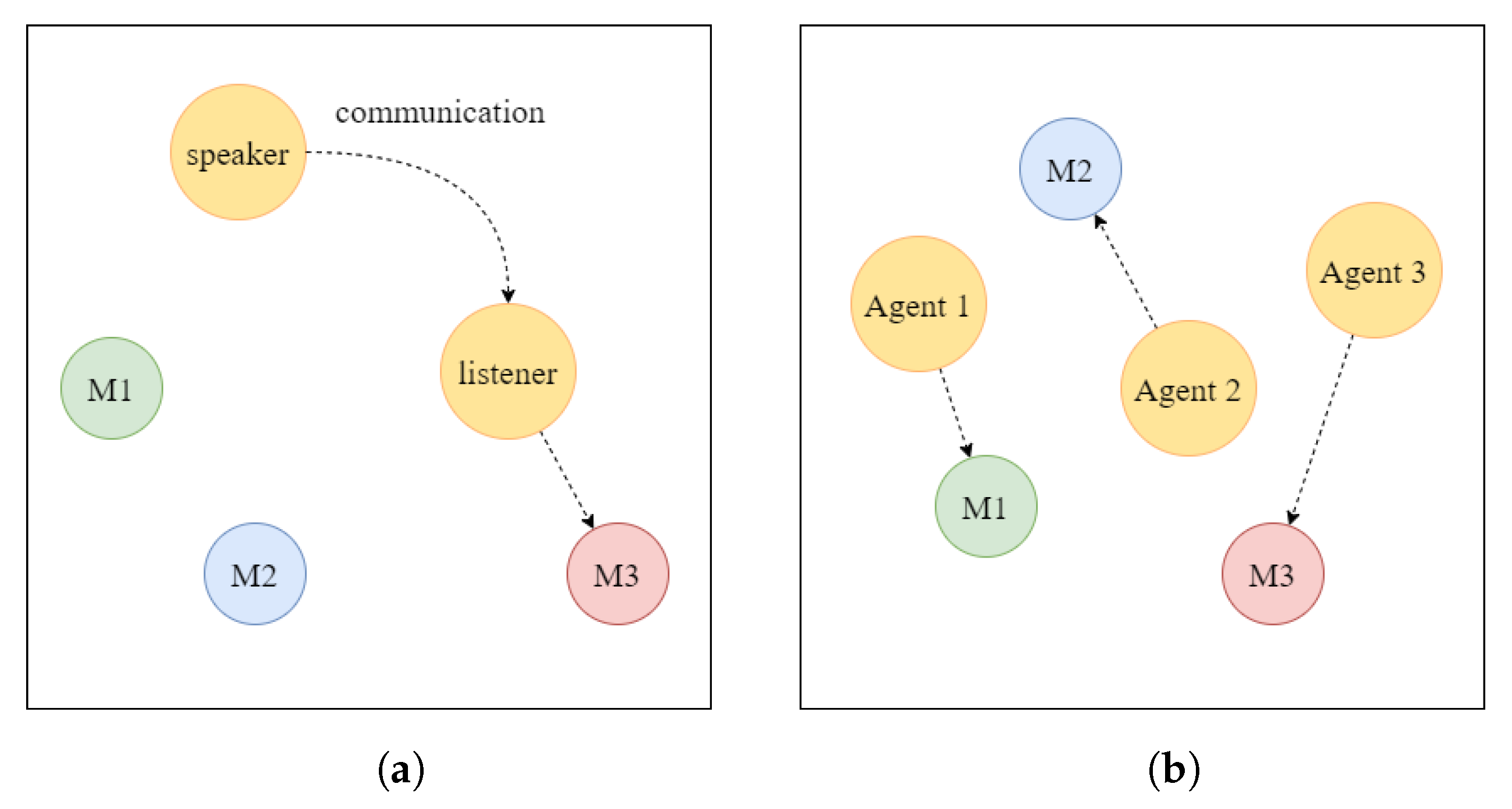
Figure 4 displays the cooperative communication task and the cooperative navigation task for the particle experiment.
Cooperative communication task: This task involves two types of cooperative agents who play the roles of speaker and listener, respectively, and there are three landmarks with different colors in the environment. In each round of the game, the listener’s objective is to reach the designated color landmark, and the reward obtained is inversely proportional to the distance from the correct landmark. The listener can obtain the relative position and color information of the landmarks, but they cannot identify the target landmark on their own. The observation information for the speaker is the color information of the target landmark, and they send messages at every moment to help the listener reach the designated landmark.
Cooperative navigation task: This task involves N cooperative types of agents and N landmarks. The aim of the task is for the N agents to move to different N landmarks, respectively, while at the same time avoiding collisions with other agents. Each agent’s observation information comprises its own and the landmarks’ relative position information and the relative position information with other agents. The reward function is calculated based on the closeness of each agent to its landmark—the closer it is, the higher the reward. Additionally, each agent actually occupies a certain physical volume and will be punished when it collides with other agents.
Under the multi-agent particle environment, the M2ATD3 algorithm proposed in this paper was compared with the MASTD3 algorithm, the previous MATD3 algorithm, and the MADDPG algorithm. Below is a presentation of the hyperparameter settings for this study. To ensure the fairness of the experiment, general parameters were set uniformly, learning rate , batch sample size . All algorithms share the same neural network structure, i.e., two fully connected layers with a width of 64 serving as the hidden layer of the policy network and Q network. The activation function of the neural network used Rectified Linear Units (Relu), and all experiments employed Adam as the optimizer of the neural network.
5.1. Q Value Estimation Bias Experiment
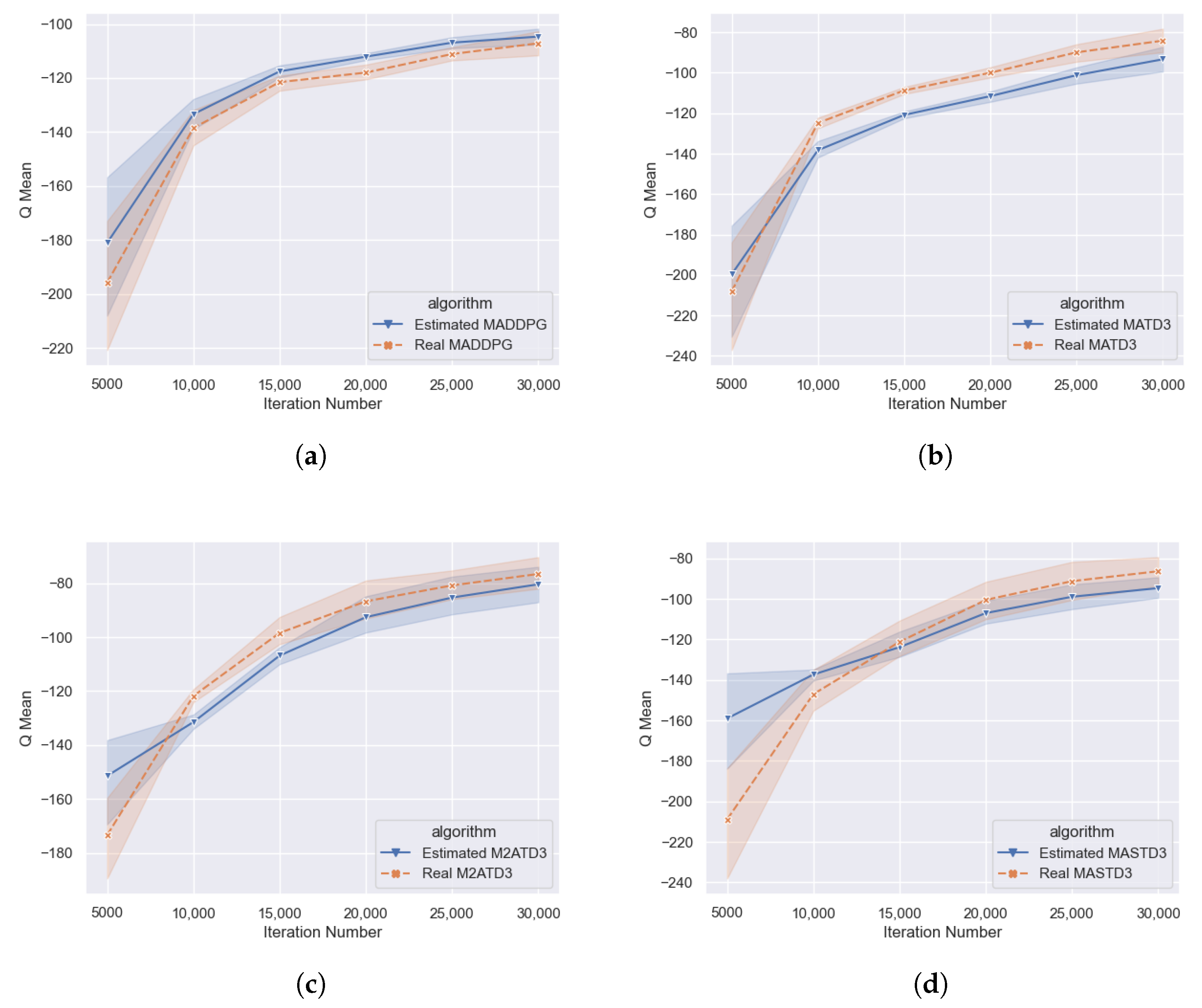
This article conducted a Q-value estimation bias experiment based on a cooperative navigation task in the particulate environment. By sampling from the experience replay pool to obtain samples of actions, states, and reward information to calculate the real Q-value and the estimated Q-value. In state s and action a, the average of 200 rounds of 100 steps’ cumulative rewards calculation is taken as the estimated value of the real Q-value. The comparison of the approximate value obtained through the Q network output with the real Q-value can reflect the situation of Q-function estimation bias of different algorithms.
As shown in
Figure 5, the lines marked with crosses represent the Q-value estimated by the neural network, and the lines marked with triangles represent the real Q-value. In the MADDPG algorithm, the blue line with the triangle logo’s Q-value is higher than the orange line, implying that the MADDPG algorithm has an over-estimation, which is more apparent in the early training; under the MATD3 algorithm, the blue line with the triangle logo’s Q-value is lower than the orange line, indicating that the MATD3 algorithm actually has an under-estimation. Under the M2ATD3, MASTD3, and other algorithms, the blue line with the triangle logo’s Q-value is lower than the orange line, which means that M2ATD3, MASTD3, and other algorithms actually have an under-estimation, and the degree of underestimation is similar to that of the MATD3 algorithm, and it can be observed that the real Q-value of MATD3, M2ATD3, MASTD3, and other algorithms are higher than the real Q-value of the MADDPG algorithm, reflecting from the side that these three kinds of algorithms’ policies are better.
The Q-value estimation bias comparative experiment can qualitatively reflect whether different algorithms have overestimation or underestimation. However, due to the complexity, randomness, and instability of multi-agent games, it is difficult to accurately calculate the true Q-values. Therefore, it is difficult for us to reliably compare the degree of Q-value underestimation of MATD3, M2ATD3, and MASTD3 algorithms, and further research is needed through performance experiments.
5.2. Algorithm Performance Experiment
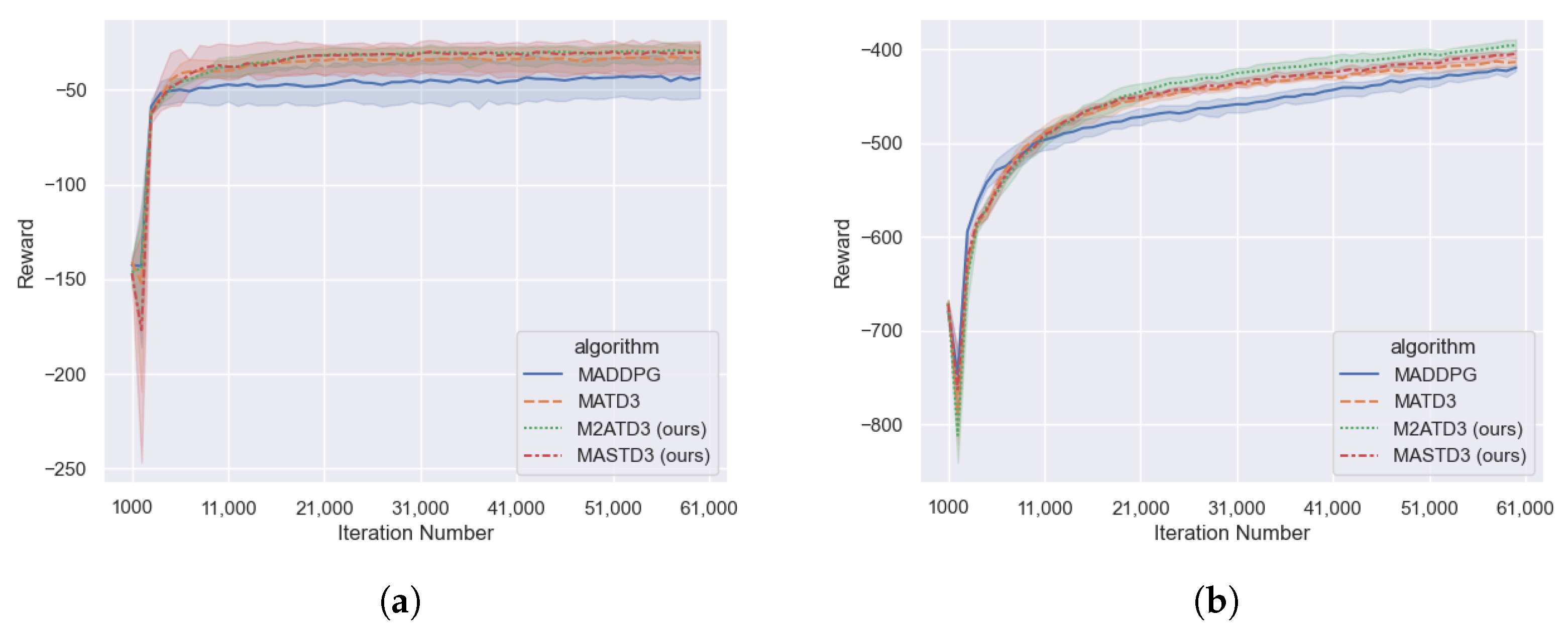
In this section, the M2ATD3 algorithm and the MASTD3 algorithm are verified with the cooperative communication task and the cooperative navigation task in the particulate environment, and compared with the MADDPG algorithm and the MATD3 algorithm. All the experiments were trained for 60,000 steps. The experiment results are as shown in
Figure 6.
As shown in
Figure 6, in the Cooperative Communication Task and the Cooperative Navigation Task, the performance of the MATD3 algorithm is superior to the MADDPG algorithm, and both the M2ATD3 algorithm and the MASTD3 algorithm have achieved higher total rewards than the MATD3 algorithm.
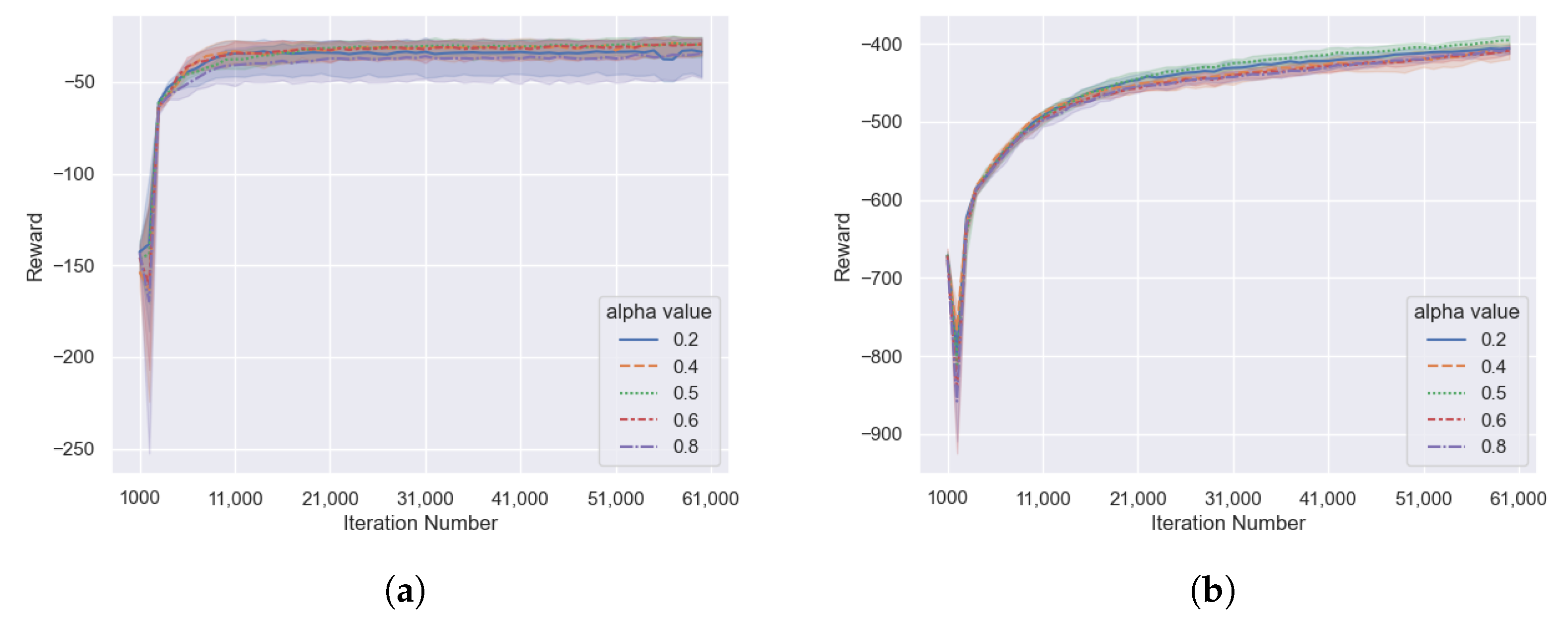
As shown in Equation (
14), hyperparameters
determine the proportion of the clipped double Q value to the average Q value when calculating the updated target value
, and select the appropriate hyperparameter
being able to balance the impact of underestimation of clipped double Q and overestimation of average Q.
As shown in
Figure 7, in the cooperative communication task and the cooperative navigation task, the M2ATD3 algorithm receives lower rewards when the
is set to 0.2 or 0.8, indicating that the low estimation of Q value caused by the clipped Double Q-Learning or the high estimation of Q value caused by the average Q value estimates will have a negative impact on the algorithm. However, the M2ATD3 algorithm receives the highest reward when the
is set to 0.5, indicating that by balancing the two Q-value estimation methods, reducing the bias in Q-value estimation can improve the performance of the algorithm.
6. Multi-Agent Tank Environment
Games have long been benchmarks and testbeds for AI research. Yunlong Lu et al. [
18] held two AI competitions of Official International Mahjong, and claim that Mahjong can be a new benchmark for AI research. In order to further investigate the performance of M2ATD3 and MASTD3 algorithms, we searched for existing reinforcement learning game environments. The Atari gaming environment [
19] is rich in content, but it is mainly a single-agent gaming environment; StarCraft [
20] and Honor of Kings [
21] are multi-agent environments, but the game state space is too large, the game randomness is too much, and the game running mechanism is protected. This places high demands on training resources and makes it difficult to set specific challenge scenarios according to research needs. Therefore, this paper referred to the classic “Tank Battle” game content and developed a multi-agent tank environment and its multi-agent reinforcement learning framework based on pygame and pytorch. This experimental environment can reflect the performance of different algorithms in real games, with suitable training scales, and can easily create different types of challenge scenarios according to research needs.
6.1. Introduction to the Multi-Agent Tank Environment
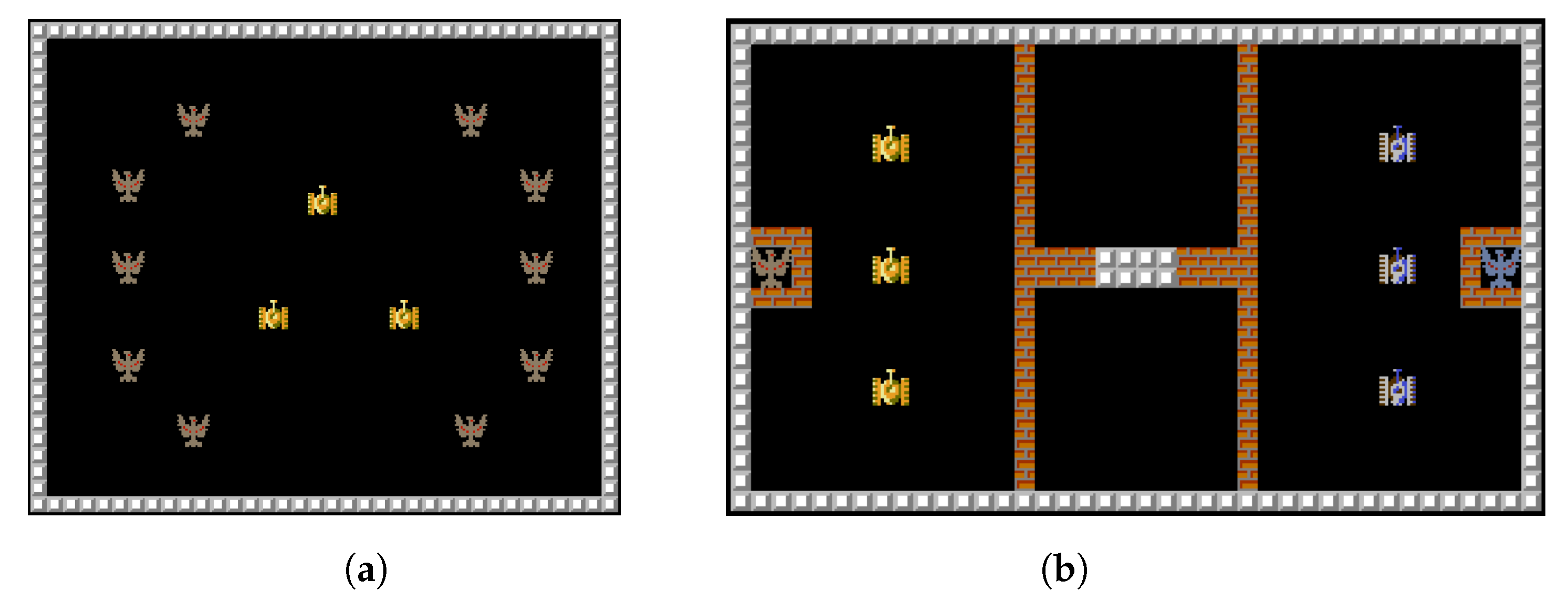
The Multi-agent Tank Environment is a game that simulates a tank battle scenario. As shown in
Figure 8, the environment is divided into two types: the scoring task and the battle task. In the scoring task, the goal is for the AI-controlled tanks to collide with as many scoring points as possible within a certain number of steps. In the battle task, the two teams of tanks win by firing bullets to destroy enemy tanks or the enemy base.
Common units in the game include: tanks, which have a certain amount of hit points (HP). When hit by a bullet, the tank will lose HP, and when the HP drops to 0, it is considered destroyed. Tanks can move and shoot. The shooting action will fire a bullet in the current direction of the tank. The bullet will be destroyed when it collides with an object or flies out of the map boundary. Bases also have a certain amount of HP. When hit by a bullet, the base will lose HP, and when the HP drops to 0, it is considered destroyed. The base cannot move. There are brick walls that can be destroyed by bullets, and stone walls that cannot be destroyed by bullets. The game map can be created and edited using xlsx format files.
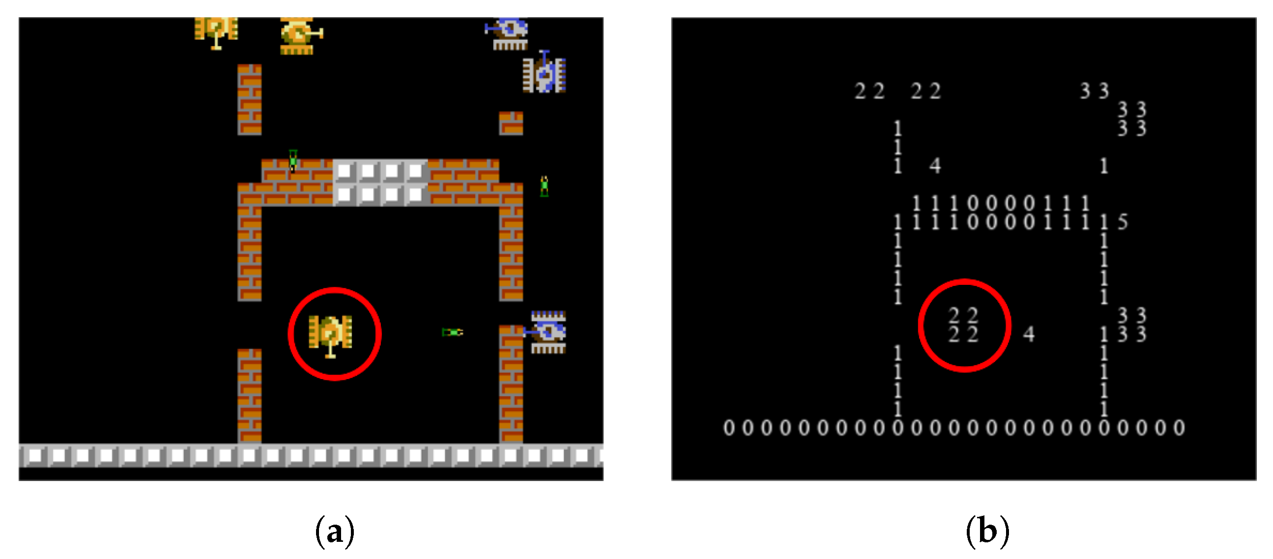
Each agent in the game can obtain local observations, which include unit features and image features. The unit features are given in the order of friendly base, friendly tank, enemy base, and enemy tank, including each unit’s survival, HP, absolute position, relative position, orientation, etc. These features are normalized. The image features use a six-channel binary image to represent whether there are stone walls, brick walls, friendly units, enemy units, friendly bullets, and enemy bullets within a 25 × 25 range near the agent. If the corresponding unit exists, the value is assigned to 1; if not, the value is assigned to 0. By using the six-channel binary image, the agent’s complete nearby situation can be depicted.
Figure 9 shows an example of graphical features of multi-agent tank environments. If the positions where the channel value is 1 are drawn as the channel index, and the positions where the value is 0 are not drawn, a complete image feature can be drawn as shown in
Figure 9b.
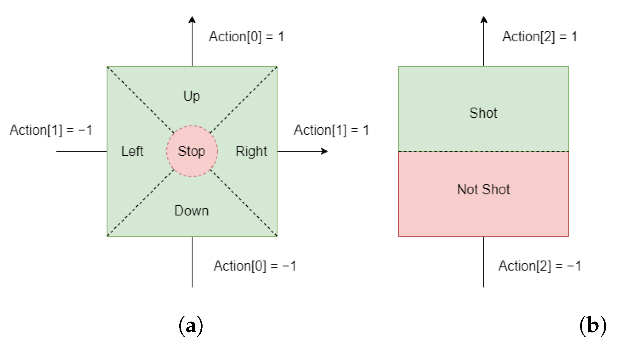
The deterministic policy of the reinforcement learning algorithm enables the agent to make decisions in a continuous action space, which is more intuitive in video games. For the deterministic policy of the reinforcement learning algorithm, we design the agent’s action space as shown in
Figure 10. We received inspiration from the way characters are controlled by the joystick in video games to design our action space for moving, as shown in
Figure 10a, where we use a 2D action to control the tank’s movement. Each movement action ranges from −1 to 1, corresponding to the joystick’s movement from left to right or from bottom to top. We determine the direction of the tank’s movement based on the maximum absolute value of the action in the horizontal or vertical direction. If the absolute value of the action in both the horizontal and vertical directions is less than 0.3, which is analogous to the joystick being in the blind area, the tank will not move. Similarly, we use a 1D action to control the tank’s shooting, as shown in
Figure 10b. The shooting action ranges from −1 to 1. When the value of the shooting action is greater than 0, the tank will shoot; otherwise, it will not shoot. The tank itself has a shooting cooldown. During the shooting cooldown, even if the agent issues a shooting action, the tank still cannot fire.
6.2. Multi-Agent Tank Environment Experiment
The process of deep reinforcement learning training using the Multi-agent Tank Environment is as follows: First, a corresponding model is created for each agent based on the selected algorithm. The model obtains actions through the policy network and interacts with the Multi-agent Tank Environment. The sequence samples obtained from the interaction are sent to the sample pool. When the samples stored in the sample pool reach a certain number, the training of the policy network and Q network of the model will start, and the model parameters will be updated at certain step intervals.
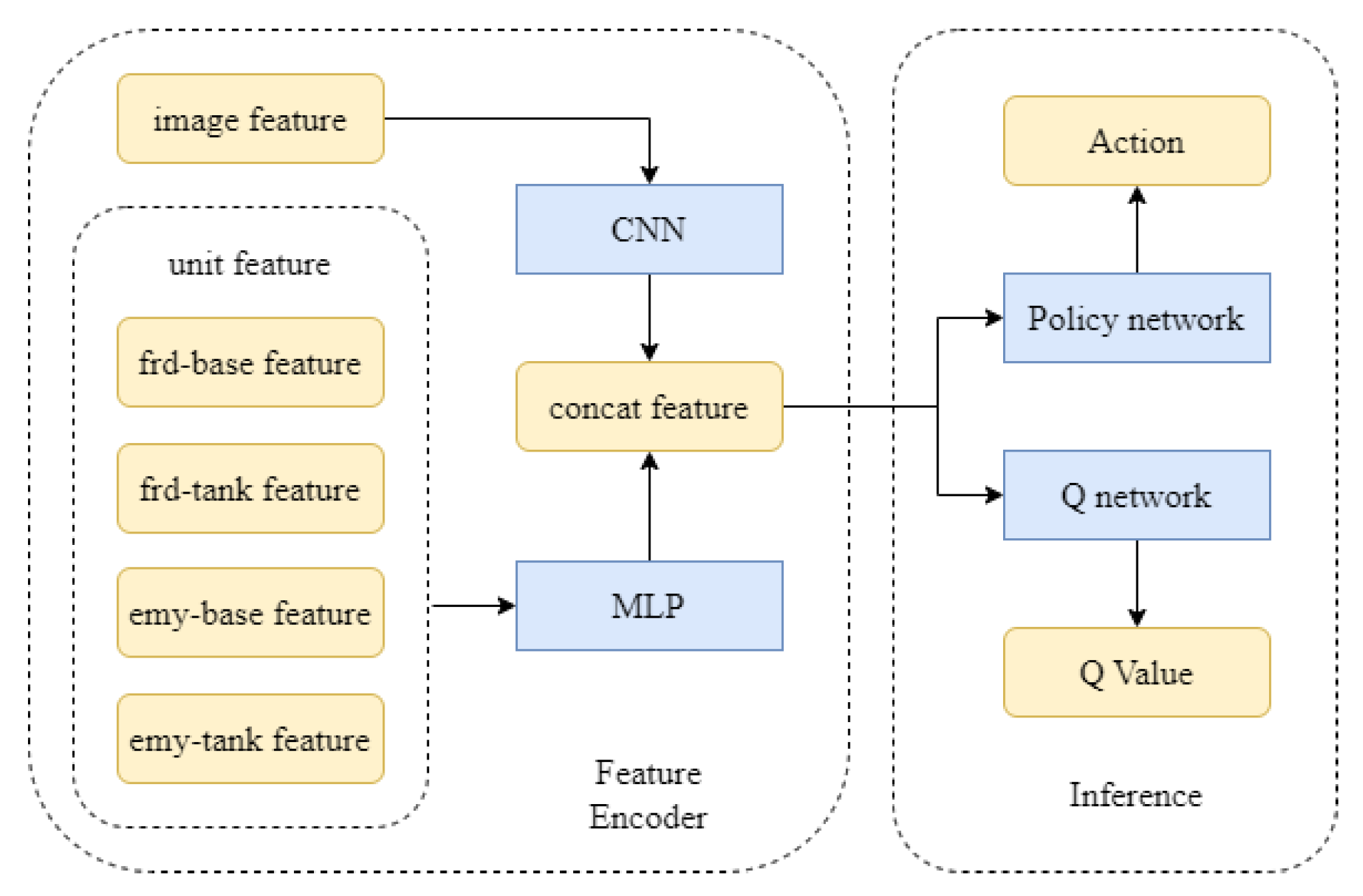
All algorithms in the experiment use the same neural network structure. A two-layer full connection layer with a width of 64 is used to process the unit features, and a convolutional neural network (CNN) is used to process the image features. The processed unit features and image features are concatenated and used as the input of the policy network and Q network. A two-layer full connection layer with a width of 64 is used as the hidden layer of the policy network and Q network. The network structure is shown in
Figure 11.
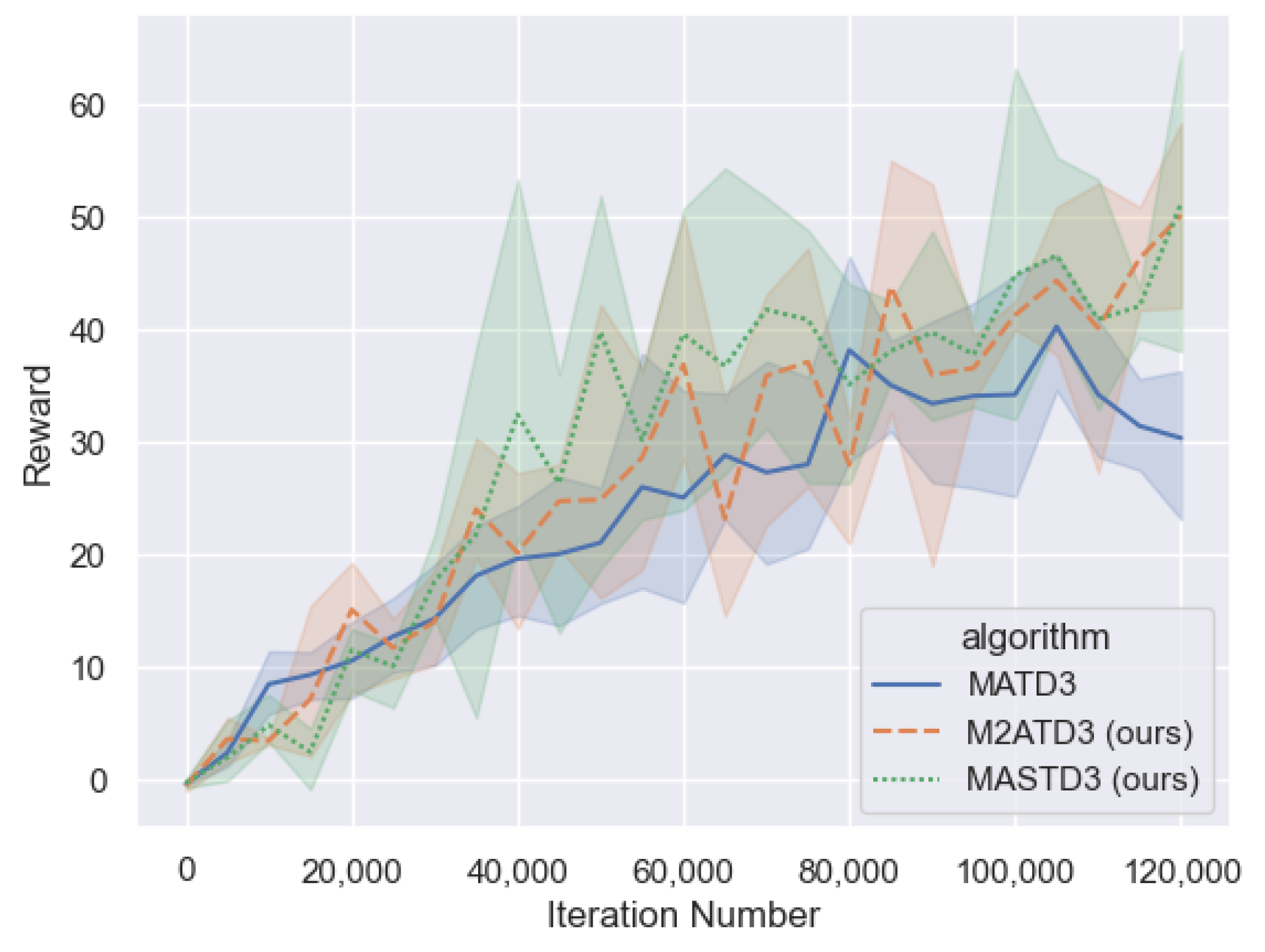
We conducted an experiment on the performance of multi-agent deep reinforcement learning algorithms in the scoring task. This task requires the AI to control three tanks to collide with as many scoring points as possible within 500 steps. There are a total of 10 optional scoring point birth positions on the map, and three positions are randomly selected each time to create scoring points. After the tank collides with a scoring point, the tank will receive a reward of +2, and a new scoring point will be created at a random other birth position. Since the reward for colliding with a scoring point is a sparse reward, we also set a dense reward according to the change in the distance from the tank to the nearest scoring point. In addition, in order to reduce the ineffective samples of the tank still moving towards the wall after colliding with the wall, we set an action mask, and set the action value in the direction of the wall to 0. The action mask effectively improves the efficiency of training.
The hyperparameters of the scoring task experiment are set as follows: learning rate
= 0.0005, discount factor
= 0.95, batch sample size N = 512. All algorithms use the same neural network structure, with the hidden layers of the policy network and Q network using two full connection layers with a width of 128. Training is conducted every 5000 steps using the current model to complete 20 evaluation rounds, and the average value of the evaluation round rewards is calculated. A total of 120,000 steps are trained, and the results are shown in
Figure 12.
The performance of the M2ATD3 algorithm and MASTD3 algorithm is better than that of the MATD3 algorithm, and they can achieve higher rewards than the MATD3 algorithm.
7. Limitations and Conclusions
7.1. Limitations
As the policy function of the agent is even more difficult to update in the correct gradient direction in the multi-agent scenario, the bias in the Q-function estimation in the multi-agent scenario can have a greater impact on policy learning compared to the single-agent scenario. Therefore, studying the bias in Q-function estimation in multi-agent scenarios is very meaningful. The M2ATD3 and MASTD3 algorithms presented in this study reduce the bias in Q-function estimation, but both algorithms have certain limitations in their application scenarios. In the M2ATD3 algorithm, each agent should have similar functions to ensure the reliability of the joint Q-value, while the application of MASTD3 in continuous action space tasks has not been deeply explored. Expanding the application scenarios of these two methods to reduce Q-function estimation bias is a direction worth further study. In addition, the unit types and task types provided by the multi-agent tank environment are relatively simple, and the content of this environment can be further enriched, providing a good experimental environment for more experiments, such as multi-agent algorithm experiments, agent cooperation with human players experiments, and so on.
7.2. Conclusions
This paper primarily studies the Q-learning of agents based on deep reinforcement learning in multi-agent scenarios, and explores methods to reduce Q-value estimation bias in multi-agent scenarios, from multi-agent reinforcement learning algorithm theory to practical model deployment.
In the theory of multi-agent reinforcement learning algorithms, the focus is on solving the bias problem of the Q-function estimation of the MADDPG algorithm and its derivative algorithm, MATD3. In the MADDPG algorithm, the Q-function evaluates the policy function, so an unbiased estimation of the Q-function helps to learn better agent strategies. This research empirically demonstrates that the MADDPG algorithm overestimates the Q-function, while the MATD3 algorithm underestimates the Q-function, and theoretically proves that bias in the MATD3 algorithm. This is followed by the introduction of the M2ATD3 and MASTD3 algorithms presented in this study to solve this problem. The M2ATD3 algorithm combines the overestimation of the Q-value brought about by the joint estimation and the underestimation brought about by the minimization operation to reduce the bias in the Q-function estimation. The MASTD3 algorithm reduces the bias in Q-function estimation by combining softmax operation with maximization operation. The two algorithms have been tested in the multi-agent particle environment and the multi-agent tank environment, proving that they can indeed solve the estimation bias problem and that agents can learn better strategies to obtain higher rewards.
In the practice of multi-agent reinforcement learning, we constructed the UESTC-tank environment. This is a tank simulation game environment with multiple units and scenes, which can generate cooperative, adversarial, and mixed mission scenarios. We focused on its scalability when building the environment, so it can support unit editing, map editing, and rule editing. We hope it can become an open and effective benchmark in the field of multi-agent reinforcement learning.

