A Quantum-Inspired Predator–Prey Algorithm for Real-Parameter Optimization

Abstract

Quantum computing has opened up various opportunities for the enhancement of computational power in the coming decades. We can design algorithms inspired by the principles of quantum computing, without implementing in quantum computing infrastructure. In this paper, we present the quantum predator–prey algorithm (QPPA), which fuses the fundamentals of quantum computing and swarm optimization based on a predator–prey algorithm. Our results demonstrate the efficacy of QPPA in solving complex real-parameter optimization problems with better accuracy when compared to related algorithms in the literature. QPPA achieves highly rapid convergence for relatively low- and high-dimensional optimization problems and outperforms selected traditional and advanced algorithms. This motivates the application of QPPA to real-world application problems.

1. Introduction

Metaheuristic optimization algorithms [1] have gained attention as a promising alternative to traditional optimization methods such as linear programming, nonlinear programming, and dynamic programming [2,3]. Metaheuristic algorithms have the ability to explore large solution spaces efficiently and handle complex problems that are difficult to model mathematically or have a large number of variables and constraints [4]. These algorithms aim to solve optimization problems by mimicking the behavior of natural processes such as biological evolution [5,6]. Some of the most prominent examples include genetic algorithms [6], which are inspired by biological evolution and natural selection, and particle swarm optimization, inspired by the behavior of a swarm of birds [7]. Another widely used form of swarm optimization is ant colony optimization, based on the behavior of ants as they forage for food [8]. Metaheuristics repeatedly create new solutions through operators such as crossover and mutation and combine them to obtain better solutions over the course of evolution (optimization) [6]. Metaheuritics are typically gradient-free optimization methods and hence suitable for models where gradient information is difficult to obtain, such as geoscientific models [9]. Since metaheuristic algorithms do not rely on gradient information, one of the major limitations is slow convergence; however, parallel implementations have been shown to address this limitation partly, for certain types of problems [9,10,11].

Apart from inspiration from biology and natural science, physics and mechanics have also inspired the design of metaheuristic optimization algorithms. Physics-based optimization algorithms are inspired by physical phenomena such as gravity, electricity, and magnetism [12,13]. These algorithms simulate the physical behavior of particles or agents in the search space to find optimal solutions. The gravitational search algorithm (GSA) [14] is based on the law of gravity and mass interactions where agents are a collection of masses that interact with each other based on Newtonian laws of motion. GSA has the advantage of being fast and easy to implement, and it is also computationally efficient when compared to related algorithms. The magnetic optimization algorithm (MOA) has a measure of the mass and magnetic field according to its fitness [15]. The fitter magnetic particles are those with larger magnetic fields and a higher mass. These particles are located in a lattice-like environment that uses the force of attraction onto their neighbors. The electromagnetism-like mechanism algorithm (EMO) is based on an attraction–repulsion mechanism to move the sample points toward optimality [16]. The chaos-based optimization algorithm (COA) [17] employs a search within nonlinear, discrete-time dynamical systems to optimize complex functions of multiple variables. It generates chaotic trajectories to systematically explore the search space, effectively seeking global minima for intricate criterion functions, and provides a dynamic strategy for nonlinear optimization challenges.

Quantum computing [18,19] has opened up various opportunities the enhancement of computational power in the coming decades. Quantum computing has the potential to provide better infrastructure for artificial intelligence [20] and also pose threats when it comes to cyber-security, as the current security systems, such as as quantum computers with enhanced computational power, are anticipated to break encryption in the future [21]. However, major challenges in the implementation of quantum computing remain [22]. Even with an implementation that is functional, the design of algorithms for quantum computing would need to be revisited [23]. There has been a growing trend in developing quantum-inspired optimization algorithms, such as the quantum genetic algorithm (QGA) [24], quantum particle swarm optimization (QPSO) [25], quantum teaching–learning-based optimization (QTLBO) [26], and the quantum marine predator algorithm (QMOA) [27]. These algorithms have shown promising results in solving optimization problems that are beyond the capabilities of classical optimization algorithms. The development of quantum optimization algorithms is expected to have a significant impact on the knapsack problem [25] and related engineering problems [26].

In this study, the term “quantum” in the algorithm’s name is attributed to its inspiration from quantum mechanics, following a naming convention employed previously [24,25,26,27], with the understanding that the algorithm is not intended for execution on real quantum computers. Inspired by quantum mechanics, we can design algorithms that do not necessarily need to wait for the development of quantum computing infrastructure. In this paper, we present the quantum predator–prey algorithm, which fuses the fundamentals of quantum computing and swarm optimization by featuring a predator–prey algorithm for real-parameter optimization. We evaluate our algorithm for sixteen benchmark real-parameter optimizations and compare prominent metaheuristic algorithms from the literature. We also provide a statistical analysis and sensitivity analysis of our results.

The rest of the paper is presented as follows. In Section 2, we provide an overview of related algorithms, and Section 3 provides the details of our proposed algorithm. Section 4 provides a discussion, and Section 5 concludes the paper.

2. Related Work

The field of metaheuristic optimization has grown rapidly with inspiration from various processes in nature. Cat swarm optimization (CSO) is a population-based optimization technique that mimics the foraging behavior of cats as they search for prey [28]. The tunicate swarm algorithm (TSA) imitates the jet propulsion and swarm behaviors of tunicates during the navigation and foraging process [29]. Bee colony optimization (BCO) [30] features the actions of individuals in various decentralized systems and is applicable to complex combinatorial optimization problems. Bacterial foraging optimization (BFO) mimics how bacteria forage over a landscape of nutrients to perform parallel non-gradient optimization [31]. Artificial bee colony (ABC) [32] is inspired by the foraging behavior of honey bees and consists of three essential components: (1.) employed foraging bees, (2.) unemployed foraging bees, and (3.) food sources. ABC has simple implementation and efficient exploration capabilities, but can become stuck in local optima and requires fine-tuning due to its sensitivity to hyperparameters [33,34].

Zervoudakis et al. [35] introduced the mayfly optimization (MO) algorithm, where the swarm of individuals are categorized as male and female mayflies and each gender exhibits distinct swarm (population) updating behavior. In the MO algorithm, individuals situated far from the best candidate or historical best trajectories move toward the optimal position at a reduced speed. On the contrary, when individuals are close to the global best candidate or historical trajectories, they move at a faster pace, which slows down the convergence rate [36]. The firefly algorithm (FA) [37] mimics the flashing behavior of fireflies to solve complex optimization problems. It suffers from some drawbacks, such as a slow convergence rate, becoming stuck in local optima, and sensitivity to the choice of hyperparameters. The dragonfly algorithm (DA) [38] originates from the static and dynamic swarming behaviors of dragonflies in nature. It can solve complex and multi-objective optimization problems and can handle constraints, while searching for diverse solutions.

The cuckoo search (CS) [39] optimization is inspired by the brood parasitism of cuckoo species with the behavior of laying eggs in the nests of other bird species. The grasshopper optimization algorithm (GOA) [40] is a multi-objective algorithm inspired by the navigation of grasshopper swarms that features the interaction of individuals in the swarm, including the attraction force, repulsion force, and comfort zone. The whale optimization algorithm (WOA) [41] mimics the social behavior of humpback whales, inspired by the bubble-net hunting strategy. The grey wolf optimizer (GWO) [42] mimics the leadership hierarchy and hunting mechanism of grey wolves in nature. Jaya [43] is a simple and parameter-less optimization algorithm designed for both constrained and unconstrained optimization. It does not require the tuning of hyperparameters, making it user-friendly. The sine cosine algorithm (SCA) [44] balances exploration and exploitation, with promising results across various domains.

In general, most of these metaheuristic optimization algorithms have the advantage of being easy to implement and providing gradient-free optimization and are suitable in problems where gradient information is not theoretically available or is computationally difficult to obtain. These are population-based algorithms that have a pool of individuals that compete and collaborate to form new solutions over time. However, they have some drawbacks, such as slow convergence, low precision in solving problems, hyperparameter tuning, and a limited ability to perform local searches. The algorithms presented earlier focus on continuous parameter optimization and can be extended to apply to discrete-parameter and constraint-parameter optimization problems.

3. Quantum Predator–Prey Algorithm

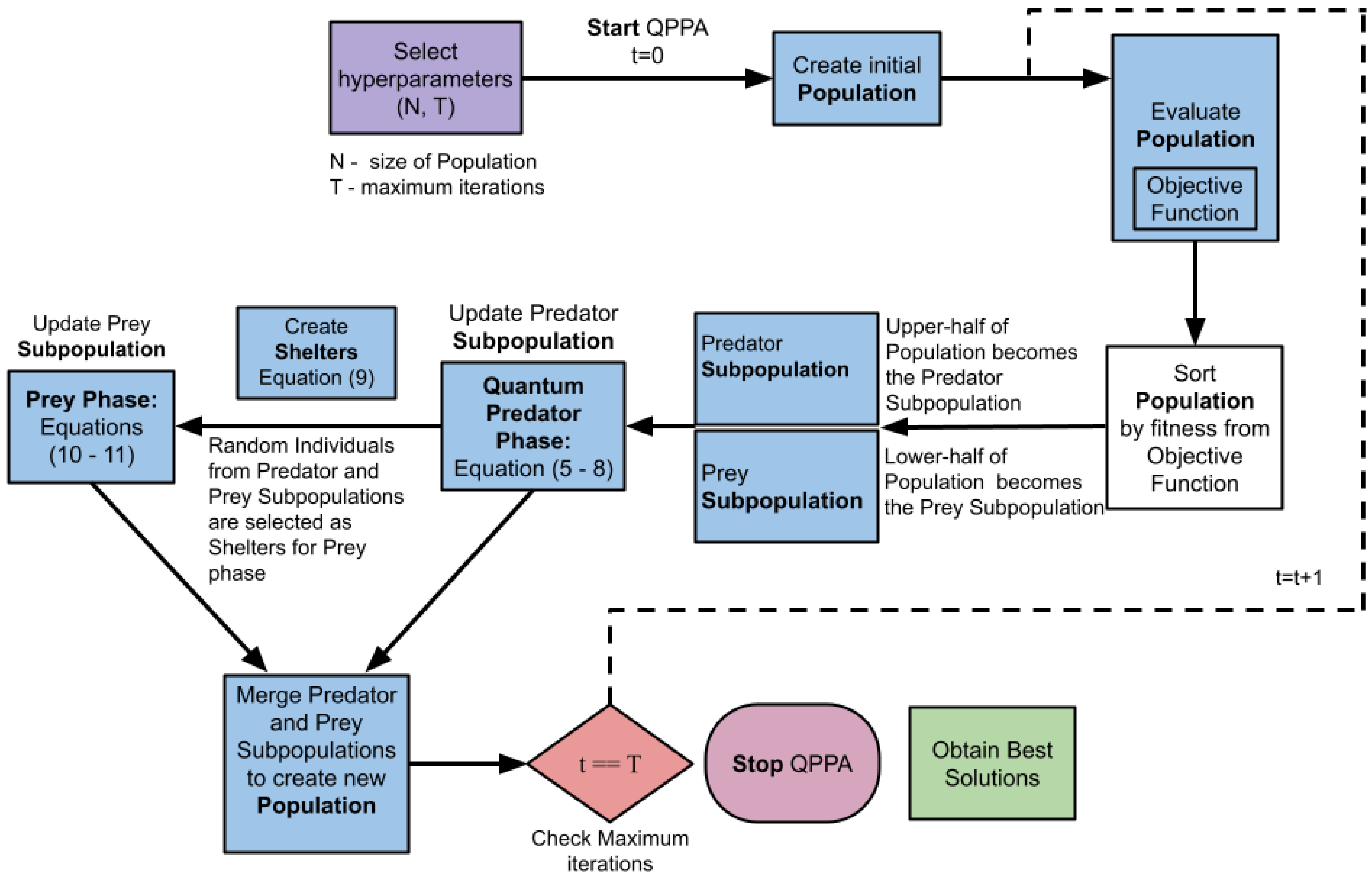
We again note that our quantum predator–prey algorithm (QPPA) combines the principles of quantum computing and swarm-based optimization. QPPA has the potential to significantly reduce the computational time, i.e., the number of iterations required to find the optimal solution, making it a promising alternative in solving computationally intensive problems.

3.1. Algorithm

We present QPPA in the framework shown in Figure 1, which is further described in Algorithm 1, featuring a population and predator and prey subpopulations. The predator subpopulation represents a process that actively seeks to improve a solution. Similar to a predator in an ecological setting hunting for prey, the predator creates better solutions by exploiting the prey subpopulation. During the process of the creation of new individuals in the population, in the first phase, we model the movement of the quantum predator toward the prey through Equations (14)–(32). We provide further details on how we derived Equation (7) in Section 3.2. Similar to an ecological setting where the prey tries to avoid capture, as shown in Figure 1, the prey hides in the shelter that is represented as a subpopulation in transition, leading to further improvement.

We begin with population X of N individuals with M decision variables (parameters) that are initialized randomly as shown in Equation (1), where $x_{i,d}$ signifies the d-th decision variable of the i-th member of the population.

$$X=\left[\begin{array}{c}{\mathbf{x}}_1\\ ⋮\\ {\mathbf{x}}_i\\ ⋮\\ {\mathbf{x}}_N\end{array}\right]=\left[\begin{array}{ccccc}{x}_{1,1}& \cdots & x_{1,d}& \cdots & x_{1,M}\\ ⋮& & ⋮& & ⋮\\ x_{i,1}& \cdots & x_{i,d}& \cdots & x_{i,M}\\ ⋮& & ⋮& & ⋮\\ x_{N,1}& \cdots & x_{N,d}& \cdots & x_{N,M}\end{array}\right]$$

(1)

We then select each individual from population X and compute the fitness score $F_i$ based on the objective function. We represent the set of fitness values for the entire population as shown in Equation (2).

$$F=\left[\begin{array}{c}{F}_1\\ ⋮\\ F_i\\ ⋮\\ F_N\end{array}\right]$$

(2)

We then sort population X based on the fitness values in increasing order. $X^{*}$ and $F^{*}$ correspond to the sorted population matrix and the sorted fitness vector, respectively, as shown in Equations (3) and (4).

$$X^{*}=\left[\begin{array}{c}{\mathbf{x}}_1^{*}\\ ⋮\\ {\mathbf{x}}_i^{*}\\ ⋮\\ {\mathbf{x}}_N^{*}\end{array}\right]=\left[\begin{array}{ccccc}{x}_{1,1}^{*}& \cdots & x_{1,d}^{*}& \cdots & x_{1,M}^{*}\\ ⋮& & ⋮& & ⋮\\ x_{i,1}^{*}& \cdots & x_{i,d}^{*}& \cdots & x_{i,M}^{*}\\ ⋮& & ⋮& & ⋮\\ x_{N,1}^{*}& \cdots & x_{N,d}^{*}& \cdots & x_{N,M}^{*}\end{array}\right]$$

(3)

$$F^{*}=\left[\begin{array}{c}{F}_1^{*}min\left(F\right)\\ ⋮\\ F_i^{*}\\ ⋮\\ F_N^{*}max\left(F\right)\end{array}\right]$$

(4)

We then update the predator subpopulation $\mathrm{\Omega }$ of $N_{pd}$ individuals and prey subpopulation $\mathrm{\Sigma }$ of $N_{py}$ individuals by dividing the sorted population $X^{*}$. The prey subpopulation consists of solutions with lower fitness values (Equation (5)), while the predator population consists of solutions with higher fitness values (Equation (6)), as highlighted in Algorithm 1 and Figure 1.

Algorithm 1 Pseudocode of QPPA

Input: decision variables, fitness function, and problem constraints. * Define hyperparameters, i.e.,  size of population N, maximum iterations T, and the number of parameters M  * Generate an initial population by drawing from a uniform distribution * Evaluate the population X using the objective function(.) for  $t=1:T$ do     (i.) Sort population X based on fitness values obtained from the objective function    (ii.) Create a prey subpopulation $\mathrm{\Omega }$ from the sorted population (lower-ranked individuals)    (iii.) Create a predator subpopulation $Sigma$ from the sorted population (higher-ranked individuals)    Quantum Predator Phase:    for  $j=1:N_{pd}$ do       Get new predator subpopulation P using Equations (7) to (10).    end for     Prey Phase:    for $j=1:N_{py}$ do       Create shelter subpopulation for the $i$th prey using Equation (11).      Get new prey subpopulation R using Equations (12) to (13).    end for  end for  Output: Get the best solution from R and P

$$\mathrm{\Omega }=\left[\begin{array}{c}{\mathrm{\Omega }}_1={\mathbf{x}}_1^{*}\\ ⋮\\ {\mathrm{\Omega }}_i={\mathbf{x}}_i^{*}\\ ⋮\\ {\mathrm{\Omega }}_{N_{py}}={\mathbf{x}}_{N_{py}}^{*}\end{array}\right]=\left[\begin{array}{ccccc}{x}_{1,1}^{*}& \cdots & x_{1,d}^{*}& \cdots & x_{1,M}^{*}\\ ⋮& & ⋮& & ⋮\\ x_{i,1}^{*}& \cdots & x_{i,d}^{*}& \cdots & x_{i,M}^{*}\\ ⋮& & ⋮& & ⋮\\ x_{N_{py},1}^{*}& \cdots & x_{N_{py},d}^{*}& \cdots & x_{N_{py},M}^{*}\end{array}\right]$$

(5)

$$\mathrm{\Sigma }=\left[\begin{array}{c}{\mathrm{\Sigma }}_1=X_{N_{py}+1}^{*}\\ ⋮\\ {\mathrm{\Sigma }}_i=X_{N_{py}+i}^{*}\\ ⋮\\ {\mathrm{\Sigma }}_{N_{pd}}=X_{N_{py}+N_{pd}}^{*}\end{array}\right]=\left[\begin{array}{ccccc}{x}_{N_{py}+1,1}^{*}& \cdots & x_{N_{py}+1,d}^{*}& \cdots & x_{N_{py}+1,M}^{*}\\ ⋮& & ⋮& & ⋮\\ x_{N_{py}+i,1}^{*}& \cdots & x_{N_{py}+i,d}^{*}& \cdots & x_{N_{py}+i,M}^{*}\\ ⋮& & ⋮& & ⋮\\ x_{N_{py}+N_{pd},1}^{*}& \cdots & x_{N_{py}+N_{pd},d}^{*}& \cdots & x_{N_{py}+N_{pd},M}^{*}\end{array}\right]$$

(6)

We now execute the quantum predator phase (Figure 1), where we update the predator subpopulation using Equation (7). In this update, we implement the analogy wherein the individuals in the predator subpopulation are chasing the individuals in the prey subpopulation. The quantum mechanism implies that an individual from the predator subpopulation can feature two copies of itself to attack the individuals from the prey subpopulation.

The constants $c1$ and $c2$ employed in Equations (7) and (8) are random variables within the range of 0–1. In the new predator subpopulation $P_{j,d}$, d denotes the decision variable of the j-th population. Similarly, in the new prey subpopulation $R_{j,d}$, d denotes the decision variable of the j-th population. Additionally, $S_{j,d}$ represents the shelter subpopulation that hosts the random individuals from the X selected by the j-th prey.

$$P_j^{new}:p{d}_{j,d}^{new}=p\pm |p{y}_{k,d}-c1·p{d}_{j,d}|ln\left(\frac{1}{c2}\right)$$

(7)

where

$$j=1:N_{pd},d=1:m,k\in 1:N_{py}$$

$$p=\frac{c_1.P{d}_{j,d}+c_2.P{y}_{k,d}}{c_1+c_2},$$

(8)

$$c_1,c_2\in rand\left(\right)$$

(9)

$$P{d}_j=\left\{\begin{array}{c}P{d}_j^{new},F_j^{pd,new}<F_j^{pd}\hfill \\ P{d}_j,else\hfill \end{array}\right.$$

(10)

In the prey phase (Figure 1), the escape of the prey to the shelter subpopulation takes place, where random individuals are taken from the predator and prey subpopulations. Note that the shelter subpopulation is the same size as the prey subpopulation, where the shelter gives a space for every individual in the prey subpopulation for refuge from the predators. It is mathematically modeled using Equations (11)–(13).

$$S_i:s_{i,d}=x_{l,d},i=1:N_{py},d=1:m,l\in 1:N,$$

(11)

$$P{y}_i^{new}:p{y}_{i,d}^{new}=p{y}_{i,d}+E·r(s_{i,d}-p{y}_{i,d})$$

(12)

where

$$i=1:N_{py},d=1:m$$

$$E=random(-2,2)$$

$$P{y}_i=\left\{\begin{array}{c}P{y}_i^{new},F_i^{py,new}<F_i^{py}\hfill \\ P{y}_i,else\hfill \end{array}\right.$$

(13)

The population continues updating using Equations (1)–(13) until the termination criteria are met.

3.2. Quantum Formulation

We give further details of the equations that have been used to create new individuals from the population in QPPA through quantum formulation via the predator and prey subpopulations. We use the foundations of quantum mechanics to formulate the quantum predator phase shown in Algorithm 1 and Figure 1.

A wave function can be solved using the Schrödinger equation [45]:

$$i\hslash \frac{\partial \mathrm{\Psi }}{\partial t}=\frac{-{\hslash }^2}{2m}\frac{{\partial }^2\mathrm{\Psi }}{{\partial }^{2}t}+V\mathrm{\Psi }$$

(14)

V is the representation of the potential energy function, h-cross (ℏ) is Plank’s constant divided by $2\pi$, and i represents an iota that gives the imaginary part of a complex number.

In order to find the probability of a particle at point x and time t, we solve $\left|\mathrm{\Psi }\right(x,t\left)\right|$. Therefore, ${\left|\mathrm{\Psi }(x,t)\right|}^{2}dx$ gives the probability of finding the particle between x and $(x+dx)$ at time t. The variable separation method [] is used to solve the Schrödinger equation.

$$\mathrm{\Psi }(x,t)=\psi \left(x\right).\phi \left(t\right)$$

(15)

The variable separation method creates two different functions dependent on x and t, respectively. Therefore, the Schrödinger equation can be written as in Equation (16):

$$i\hslash \frac{1}{\phi }\frac{\partial \phi }{\partial t}=\frac{-{\hslash }^2}{2m}\frac{1}{\psi }\frac{{\partial }^2\psi }{{\partial }^{2}t}+V$$

(16)

The second part of the above equation is dependent on x and independent of t and is therefore called the time-independent Schrödinger equation. The specification of the potential function $V\left(x\right)$ is important to solve the Schrödinger equation. Some of the most common potential functions are the one-dimensional delta potential well, the harmonic oscillator, and the square potential well. In our algorithm, we use the delta potential function, and therefore we define the Dirac delta function $\delta \left(x\right)$ as in Equation (17).

$$\delta \left(x\right)=\left\{\begin{array}{c}0,x\ne 0\hfill \\ \infty ,x=0\hfill \end{array}\right.,with{\int }_{-\infty }^{+\infty }\delta \left(x\right)dx=1$$

(17)

$\delta (x-c)$ is a similar function that has the same properties at position c as the origin in $\delta \left(x\right)$. If we multiply $\delta (x-c)$ by an ordinary function $f\left(x\right)$, it is the same as multiplying $f\left(c\right)$.

$$f\left(x\right)\delta (x-c)=f\left(c\right)\delta (x-c)$$

(18)

Integrating both sides from −∞ with ∞, we obtain $f\left(c\right)$, where c is a constant.

$${\int }_{+\infty }^{-\infty }f\left(x\right)\delta (x-c)dx={\int }_{+\infty }^{-\infty }f\left(c\right)\delta (x-c)dx$$

(19)

We can consider the potential of the form of Equation (20):

$$V\left(x\right)=-c\delta \left(x\right).$$

(20)

Replacing the potential function in a time-independent Schrödinger equation, we have Equation (21):

$$\frac{-{\hslash }^2}{2m}\frac{1}{\psi }\frac{{\partial }^2\psi }{{\partial }^{2}t}-c\delta \left(x\right)\psi =E\psi$$

(21)

which can be written in the form given in Equation (22):

$$\frac{1}{\psi }\frac{{\partial }^2\psi }{{\partial }^{2}t}+k^2\psi =0.$$

(22)

where

$$k=\sqrt{\frac{-2mE}{{\hslash }^2}}.$$

(23)

This potential yields both bound states $(E<0)$ and scattering states $(E>0)$. In the region $x<0$, $V\left(x\right)=0$, and E is negative by assumption, so k is real and positive, and hence we obtain Equation (24).

$$\psi =A{e}^{kx},x<0$$

(24)

In Equation (24), we assume that the pre-exponential factor is kept at 0 for the negative x part, for which the power of exponential would be $-kx$, as it would blow up when $x\to -\infty$.

In the region $x>0$, $V\left(x\right)=0$, we obtain Equation (25):

$$\psi =B{e}^{-kx},x>0$$

(25)

The above equation does not include the term whose power of exponential is $kx$ because it would blow up as $x\to \infty$, so the pre-exponential factor is kept at 0. On keeping $A=B$, we obtain a general formula:

$$\psi \left(x\right)=\left\{\begin{array}{c}B{e}^{kx},x<0\hfill \\ B{e}^{-kx},x>0\hfill \end{array}\right.$$

(26)

We assume that the particle is present in a one-dimensional space. We refer to point p as the local attractor that is at the center of the potential well. Equation (27) represents the potential energy of the particle in a one-dimensional delta potential well.

$$\psi \left(x\right)=-a\delta (x-p)=-a\delta \left(y\right)$$

(27)

Let m denote the mass of the particle and $x-p=y$. Below are the steps involved in integrating the Schrödinger equation from $-\epsilon$ to $+\epsilon$.

$${\int }_{-\epsilon }^{+\epsilon }(\frac{\hslash }{2m}\frac{d^2\psi \left(y\right)}{d{y}^2}-a\delta \left(y\right)\psi \left(y\right))dy={\int }_{-\epsilon }^{+\epsilon }\left(E\psi \left(y\right)\right)dy=0$$

taking the limit as $\epsilon$ goes to 0,

$${\psi }^{,}\left(0^{+}\right)-{\psi }^{,}\left(0^{-}\right)=-\alpha \frac{2m}{{\hslash }^2}\psi \left(0\right)$$

$$2Bk=-\alpha \frac{2m}{{\hslash }^2}B$$

$$E=E_o=-\frac{{\hslash }^2{k}^2}{2m}=-\frac{a^{2}m}{2{\hslash }^2}$$

We integrate ${\left|\psi \left(x\right)\right|}^2$ to determine the constants

$${\int }_{-\infty }^{+\infty }{\left|\psi \left(y\right)\right|}^{2}dx=\frac{B^2}{k}=1$$

$$B=\sqrt{k},L=\frac{1}{k}=\frac{{\hslash }^2}{2m}$$

(28)

where L is the length of the potential well; therefore, the $\psi \left(y\right)$ represents the normalized wave function as given in Equation (29).

$$\psi \left(y\right)=\frac{1}{\sqrt{L}}{e}^{-\frac{\left|y\right|}{L}}$$

(29)

We assume that s is a random number in the range (0, 1/L) and s is the probability of the existence of a quantum body in a particular position p, as given in Equation

$$s=random(0,\frac{1}{L})=\frac{1}{L}random(0,1)=u.\frac{1}{L}$$

u is a random number in the interval (0,1).

$$s={\left|\psi \left(x\right)\right|}^2=\frac{1}{L}{e}^{-\frac{\left|2y\right|}{L}}$$

$$u=e^{-\frac{\left|2y\right|}{L}}\to \left|y\right|=\pm \frac{L}{2}ln(\frac{1}{u})-p=\pm \frac{L}{2}ln(\frac{1}{u})$$

(30)

where p is the local attractor used to define a new random location between the best and current solution for better diversification in each iteration, which increases the exploratory tendency of the optimization technique.

$$L=2|py-c1·pd|$$

(31)

$$c1\in rand\left(\right)$$

We substitute Equation (30) with Equation (31) and obtain the following equation to update the position of the particles.

$$p{d}^{new}=p\pm |py-c1·p{d}^{old}|ln(\frac{1}{c2})$$

(32)

$p{d}^{old}$ and $p{d}^{new}$ are the solutions before and after updating, respectively.

4. Empirical Evaluation

4.1. Experimental Settings

We assess the efficacy of QPPA for selected real-parameter optimization benchmark problems and compare it with related algorithms from the literature. We first outline the experimental configuration employed to evaluate the performance of the selected algorithms. We select a set of fourteen benchmark objective functions, as shown in

Table 1. Benchmark objective functions from Congress on Evolutionary Computation, 2022.

Function	Name	Formulation	Search Space
F1	Zakharov	${\mathrm{\Sigma }}_{i=1}^D{x}_i^2+{\left({\mathrm{\Sigma }}_{i=1}^{D}0.5i{x}_i\right)}^2+{\left({\mathrm{\Sigma }}_{i=1}^{D}0.5i{x}_i\right)}^4$	[−100, 100]
F2	Rosenbrok	${\mathrm{\Sigma }}_{i=1}^{D-1}[100{(x_{i+1}-x_i^2)}^2+{(x_i-1)}^2]$	[−10, 10]
F3	Exp. Schaffer	$g(x,y)=0.5+\frac{({sin}^2\left(\sqrt{x^2+y^2}\right)-0.5)}{{(1+0.001(x^2+y^2))}^2}$	[−100, 100]
		$f\left(x\right)=g(x_1,x_2)+g(x_2,x_3)+\dots +g(x_{D-2},x_{D-1})+g(x_{D-1},x_D)$
F4	Rastrigin	$10D+{\mathrm{\Sigma }}_{i=1}^D[x_i^2-10cos\left(2\pi x_i\right)]$	[−100, 100]
F5	Levy	${sin}^2\left(\pi w_1\right)+{\sum }_{i=1}^{D-1}{\left(w_i-1\right)}^2\left[1+10{sin}^2(\pi w_i-1)\right]+{\left(w_D-1\right)}^2\left[1+{sin}^2\left(2\pi w_D\right)\right]$	[−30, 30]
		$w_i=1+\frac{x_{i-1}}{4}$, $\forall i=1,\dots ,D$
F6	Bent Cigar	$x_i^2+{10}^{6{\sum }_{i=2}^D{x}_i^2}$	[−100, 100]
F7	HGBat	${\left|{\left({\sum }_{i=1}^D{x}_i^2\right)}^2-{\left({\sum }_{i=1}^D{x}_i\right)}^2\right|}^{0.5}+\frac{0.5{\sum }_{i=1}^D{x}_i^2+{\sum }_{i=1}^D{x}_i}{D}+0.5$	[−1.28, 1.28]
F8	High Conditioned Elliptic	${\sum }_{i=1}^D{\left({10}^6\right)}^{\frac{i-1}{D-1}}{x}_i^2$	[−500, 500]
F9	Happycat	${\left|{\sum }_{i=1}^D{x}_i^2-D\right|}^{1/4}+\frac{\left(0.5{\sum }_{i=1}^D{x}_i^2+{\sum }_{i=1}^D{x}_i\right)}{D}+0.5$	[−32, 32]
F10	Modified Schwefel	$418.9829\times D-{\sum }_{i=1}^{D}g\left(z_i\right)$	[−50, 50]
		$z_i=x_i+4.209687462275036E+002$
F11	Ackley	$-20exp\left(-0.2\sqrt{\frac{1}{D}{\sum }_{i=1}^D{x}_i^2}\right)-exp\left(\frac{1}{D}{\sum }_{i=1}^{D}cos\left(2\pi x_i\right)\right)+20+e$	[−50, 50]
F12	Discus	${10}^6{x}_1^2+{\sum }_{i=2}^D{x}_i^2$	[−65.536, 65.536]
F13	Griewank	${\mathrm{\Sigma }}_{i=1}^D\frac{x_i^2}{4000}-{\Pi }_{i=1}^{D}cos(\frac{x_i}{\sqrt{i}})+1$	[−5, 5]
F14	Schaffer	${\left[\frac{1}{D-1}{\sum }_{i=1}^{D-1}\left(\sqrt{s_i}·\left(sin\left(50.0s_i^{0.2}\right)+1\right)\right)\right]}^2,$	[−5, 5]
		$s_i=\sqrt{x_i^2+x_{i+1}^2}$

, which provides the function name, formulation, and search space. We compare QPPA with established optimization methods from the literature using the hyperparameters given in their original papers, as shown in shown in

Table 2. Hyperparameters for the selected optimization algorithms from the literature.

Algorithm	Hyperparameters	Values
PSO [7]	Cognitive and social constant	(c1, c2) ∈ (2, 2)
	Inertia weight	0.99
	Velocity limit	Dimension range
GA [6]	Type	Real coded
	Mutation rate	0.1
	Crossover	Whole arithmetic
GSA [14]	Control parameter	100
	Alpha	20
	$R_{Norm}$	2
	$R_{Power}$	1
SCA [44]	Constant hyperparameter	2
	Probability switch	0.5
Jaya [43]	No Parameters
GWO [42]	Convergence parameter (a)	a: Linear reduction from 2 to 0.
MA [35]	Inertia Weight	0.8
	Inertia Weight Damping Ratio	1
	Personal Learning Coefficient	$a_1=1$
	Global Learning Coefficient	$a_2=1.5,a_3=1.5$
	Random Flight	1
	Distance Sight Coefficient	2
LSA [46]	Channel Time	0

. We make an exception for the case of PSO for the F7 objection function (HGBat) given in Table 1, where we fine-tune the hyperparameters in trial experiments.

In our algorithmic analysis, we investigate two different settings. In Setting 1, we focus on evaluating the algorithm’s efficiency and convergence behavior in a lower-dimensional solution space. Hence, in Setting 1, we use a population size ($N_p=30$), maximum iterations ($T=1000$), and dimension ($D=10$). In Setting 2, we maintain a consistent population size ($N_p=30$) and iteration count ($T=1000$) and consider a much higher-dimensional space ($D=100$). This choice allows us to showcase the algorithm’s scalability and robustness when solving more complex, high-dimensional optimization problems. By systematically varying these settings, we aim to comprehensively understand the algorithm’s strengths and limitations across a wide range of optimization scenarios.

4.2. Results

We report the performance results of the respective optimization algorithms using two indicators: the fitness score of the average of the best (quasi-optimal) solutions and the standard deviation (st. dev) of the best solutions. We present the results in

Table 3. Results of optimization algorithms on objective functions in Setting 2 ($D=10$). We highlight the best results in bold.

Function	QPPA	PSO	GA	GSA	SCA	Jaya	GWO	MA	LSA
F1	0.00E+00	1.17E+04	5.01E−21	5.93E−18	1.73E−22	1.89E+04	1.50E−109	9.79E−105	8.06E−84
St. dev	0.00E+00	3.51E+03	7.43E−21	1.81E−18	4.88E−22	7.37E+03	4.58E−109	3.10E−104	2.55E−83
F2	8.45E−02	9.60E+01	8.15E+00	5.45E+00	7.07E+00	2.02E+00	6.57E+00	1.03E−10	9.62E+00
St. dev	2.06E−01	1.55E+04	1.31E+00	2.72E−01	2.39E−01	1.47E+00	6.95E−01	3.25E−10	1.92E+01
F3	0.00E+00	3.97E+00	4.51E−01	2.12E+00	4.99E−01	3.34E+00	4.63E−01	1.50E−02	1.39E+00
St. dev	0.00E+00	1.02E−01	4.72E−01	4.85E−01	5.21E−01	2.99E−01	5.38E−01	4.60E−02	6.33E−01
F4	0.00E+00	5.69E+01	0.00E+00	3.33E+01	4.15E−01	5.97E−01	1.80E+01	8.82E−01	1.47E+01
St. dev	0.00E+00	1.31E+03	1.91E+00	1.06E+01	1.31E+00	1.88E+00	1.43E+01	2.56E−01	1.12E+01
F5	1.50E−32	1.17E−01	7.42E−01	3.89E−19	3.24E−01	3.33E+01	3.13E−07	2.77E−30	3.98E+00
St. dev	0.00E+00	2.60E+01	2.07E−17	1.76E−19	1.74E−01	1.06E+01	1.29E−07	8.76E−30	4.10E+00
F6	0.00E+00	3.84E−07	2.31E−17	2.84E+02	1.65E−21	9.49E−08	8.85E−113	8.36E−112	3.71E−106
St. dev	0.0E+00	9.82E+08	4.24E−01	3.65E+02	5.20E−21	7.60E−08	1.20E−112	2.64E−111	1.17E−105
F7	4.59E−01	1.36E−02	4.20E−01	4.55E−01	2.58E−01	2.61E−01	3.75E−01	4.71E−02	3.53E−01
St. dev	8.17E−02	4.20E−02	6.65E−02	4.69E−02	5.21E−02	5.21E−02	7.94E−02	1.49E−01	6.54E−02
F8	0.00E+00	1.02E+07	3.86E−18	1.54E+06	6.19E−22	1.83E−08	1.50E−113	2.39E−96	2.84E−107
St. dev	0.0E+00	7.22E+08	5.13E−18	2.78E+06	1.92E−21	2.66E−08	1.71E−113	7.55E−96	8.89E−107
F9	2.78E−01	0.51E+01	0.32E+01	3.13E+00	3.02E+00	0.69E+02	3.11E+00	3.27E−01	2.96E+00
St. dev	4.68E−16	0.18E+02	8.10E−02	1.03E−01	2.32E−01	0.24E+02	2.75E−01	1.04E+00	2.14E−01
F10	3.77E+03	3.77E+03	3.77E+03	3.77E+03	3.77E+03	3.77E+03	3.77E+03	3.77E+02	3.77E+03
St. dev	0.00E+00	2.64E−06	0.00E+00	0.00E+00	0.00E+00	0.00E+00	0.00E+00	1.19E+03	0.00E+00
F11	4.44E−16	0.19E+02	3.21E−12	3.16E−09	1.99E+01	0.19E+02	2.01E+00	1.47E−15	1.30E+00
St. dev	0.00E+00	8.20E−02	3.01E−12	2.85E−10	4.60E−02	6.36E+00	4.63E−15	1.05E+00	6.53E−03
F12	0.00E+00	2.16E+00	4.31E−22	7.66E+02	5.73E−05	6.04E−13	6.46E−115	1.47E−15	1.66E−113
St. dev	0.00E+00	7.29E+03	6.31E−22	2.23E+02	4.35E−03	3.40E−13	1.90E−114	4.63E−15	5.24E−113
F13	0.00E+00	5.48E−02	3.00E−03	0.00E+00	3.36E−02	8.32E−02	1.79E−02	6.66E−17	5.83E−03
St. dev	0.00E+00	5.60E−02	1.00E−02	0.00E+00	3.11E−01	7.70E−02	2.16E−02	2.11E−16	1.36E−02
F14	1.48E−15	2.48E−04	1.70E−02	3.00E−03	9.89E−02	2.70E−04	2.23E−02	9.07E−32	5.87E−05
St. dev	4.68E−15	1.12E−04	3.60E−02	1.00E−02	5.11E−02	1.78E−04	3.11E−02	2.87E−31	1.85E−04

, which compares our QPPA with well-known optimization methods, including PSO [7], real-coded GA [6], GSA [14], SCA [44], Jaya [43], GWO [42], MA [35], and LSA [46]. The reported mean and standard deviation values are outcomes derived from five independent runs.

We find that QPPA is demonstrated to be the strongest performer in 12 out of 14 functions in Setting 1, as shown in Table 3. The algorithm’s ability to adapt effectively and find a balance between exploring new possibilities and exploiting promising ones allows it to navigate complex search landscapes efficiently, which leads to optimal or near-optimal solutions. Although MA stands out in problems such as HGBat, Katsuura, and Modified Schwefel, QPPA’s widespread success across a diverse set of functions highlights its potential as a versatile optimization method.

We further provide the results for a more complex case (Setting 2) in

Table 4. Results of optimization algorithms on objective functions in Setting 2 ($D=100$). We highlight the best results in bold.

Function	QPPA	PSO	GA	GSA	SCA	Jaya	GWO	MA	LSA
F1	1.73E−304	2.77E+05	1.63E+03	1.13E+04	1.59E+05	1.64E+11	7.18E+04	1.07E+05	1.30E+05
F2	9.80E+01	2.61E+03	9.41E+05	1.61E+03	3.95E+05	1.55E+07	9.82E+01	9.69E+01	7.07E+02
F3	0.00E+00	4.45E+01	3.46E+01	1.79E+01	4.14E+01	4.85E+01	2.22E+01	3.21E+01	3.96E+01
F4	0.00E+00	2.68E+02	1.62E+03	1.43E+03	9.31E+03	2.73E+05	4.55E−13	1.27E+03	2.56E+02
F5	1.14E+01	9.19E+01	2.95E+02	2.22E+01	9.01E+02	7.67E+03	2.29E+01	4.34E+01	4.70E+02
F6	0.00E+00	3.49E+07	7.16E+08	7.68E+08	6.91E+08	2.92E+11	2.75E−24	8.26E+00	1.94E+06
F7	4.99E−01	8.57E−01	7.21E+02	7.04E−01	5.12E−01	4.53E+01	7.70E−01	1.55E−06	4.28E−01
F8	0.00E+00	3.09E+05	2.54E+07	4.53E+09	3.69E+07	4.91E+11	2.38E−25	1.47E+07	4.20E+05
F9	6.16E−01	6.15E+00	3.07E−01	5.61E−01	2.94E+00	3.26E+02	5.96E−01	5.58E−01	5.36E−01
F10	1.27E−03	5.19E+00	9.25E+01	8.20E+00	1.15E+02	8.22E+03	1.27E−03	1.27E−03	6.14E−03
F11	4.44E−16	3.31E+00	9.83E+00	4.56E+00	2.06E+01	1.99E+01	2.10E−13	8.06E+00	1.94E+01
F12	0.00E+00	3.52E+01	1.10E+03	3.55E+03	3.18E+03	4.58E+06	1.07E−29	6.70E−01	3.70E+01
F13	0.00E+00	3.94E−01	1.18E+00	2.36E+02	0.35E+00	1.17E+00	0.1E+00	5.01E−08	1.8E−03
F14	1.93E−91	9.53E−02	3.67E+00	5.36E−02	1.16E+00	2.63E−04	9.13E−04	4.15E−03	5.34E−02

. In Setting 2, we observe that QPPA demonstrates superior performance by outperforming all other algorithms in 13 out of 14 functions. Notably, MA surpasses QPPA in optimizing the Happycat function. These findings underscore the commendable performance of QPPA, particularly in the realm of higher-dimensional problems.

We present a statistical analysis to evaluate the significance of QPPA using an unpaired t-test [47] of the results from Setting 1. An unpaired t-test, also known as an independent t-test, compares the means of two unrelated groups to determine whether there is a noteworthy difference between them. We can determine whether the difference is statistically significant or whether it occurs by chance alone.

Table 5. p-values for the t-test for the effectiveness of the respective algorithms coupled with QPPA (e.g., PSO vs. QPPA) in Setting 1 ($T=1000$, $D=10$, $N_p=30$).

Function	PSO	GA	GSA	SCA	Jaya	GWO	MA	LSA
F1	2.61E−05	1.12E−19	1.33E−16	3.87E−21	4.23E−05	3.35E−108	2.19E−103	1.80E−82
F2	1.03E−06	1.80E−02	1.19E−02	1.56E−02	4.33E−01	1.45E−02	1.88E−01	2.13E−02
F3	8.87E−01	1.01E−01	4.74E−01	1.12E−01	7.46E−01	1.03E−01	3.29E−01	3.09E−01
F4	1.27E−05	0.00E+00	7.44E−02	9.27E−01	1.33E−01	4.03E−02	1.97E−01	3.29E−02
F5	2.61E−03	1.66E−01	8.70E−18	7.24E−01	7.45E−02	7.00E−06	6.16E−29	8.89E−01
F6	8.58E−10	5.17E−16	6.35E−03	3.69E−20	2.12E−06	1.98E−111	1.87E−110	8.30E−105
F7	7.22E−01	8.65E−01	9.63E−02	4.49E−01	4.41E−01	1.86E−01	9.21E−01	2.36E−01
F8	2.28E−10	8.63E−17	3.44E−07	1.38E−20	4.09E−07	3.35E−112	5.34E−95	6.35E−106
F9	1.07E−03	5.73E−01	3.29E−01	5.67E−01	1.48E−03	3.80E−01	6.59E−01	6.91E−01
F10	0.00E+00	0.00E+00	0.00E+00	0.00E+00	0.00E+00	0.00E+00	7.59E−04	0.00E+00
F11	5.90E−05	7.18E−11	7.07E−08	4.45E−02	4.47E−02	4.49E−01	2.29E−14	2.91E−01
F12	4.83E−05	9.64E−21	1.71E−04	1.28E−03	1.35E−11	1.44E−113	3.29E−14	3.71E−112
F13	1.22E−01	7.17E−02	0.00E+00	7.51E−01	1.86E−01	0.40E+00	1.49E−15	0.13E+00
F14	5.54E−03	3.79E−01	7.14E−01	2.21E−01	6.04E−03	4.98E−01	3.31E−14	1.31E−03

presents the outcomes (p-values) of the unpaired t-test performed between QPPA and the other algorithms, where we use a threshold value of 0.02 to determine whether QPPA is significantly better. Based on the results, we find that QPPA provides better performance than PSO, Real-GA, GSA, SCA, Jaya, GWO, MA, and LSA.

Table 6. Iteration-wise results for QPPA in Setting 2 ($T=1000$, $D=100$, $N_p=30$).

Func.	Iter. 0	Iter. 100	Iter. 200	Iter. 300	Iter. 400	Iter. 500	Iter. 600	Iter. 700	Iter. 800	Iter. 900	Iter. 1000
F1	1.639E+11	2.33E−26	8.76E−60	3.35E−92	3.98E−125	2.68E−150	4.70E−170	4.14E−214	3.23E−242	2.00E−275	1.85E−302
F2	2.07E+03	9.82E+01	9.81E+01	9.73E+01	9.64E+02	9.55E+01	9.34E+01	9.32E+01	9.25E+01	9.24E+01	9.15E+01
F3	2.07E+03	1.73E−14	0.00E+00	0.00E+00	0.00E+00	0.00E+00	0.00E+00	0.00E+00	0.00E+00	0.00E+00	0.00E+00
F4	2.02E+03	0.00E+00	0.00E+00	0.00E+00	0.00E+00	0.00E+00	0.00E+00	0.00E+00	0.00E+00	0.00E+00	0.00E+00
F5	2.08E+10	1.72E+01	1.35E+01	1.20E+01	1.12E+01	1.12E+01	1.11E+01	1.11E+01	1.04E+01	0.00E+00	0.00E+00
F6	2.08E+10	1.86E−29	7.17E−68	2.16E−105	2.05E−144	3.54E−177	3.43E−214	3.45E−254	7.71E−289	0.00E+00	0.00E+00
F7	2.27E+03	5.00E−01	4.30E−01	4.30E−01	4.30E−01	4.30E−01	4.30E−01	4.30E−01	4.30E−01	4.30E−01	4.30E−01
F8	2.27E+03	5.91E−29	7.95E−68	1.80E−109	1.62E−163	2.76E−216	1.56E−258	7.65E−292	0.00E+00	0.00E+00	0.00E+00
F9	2.27E+03	7.56E−01	6.95E−01	6.05E−01	5.45E−01	5.45E−01	5.45E−01	5.45E−01	5.45E−01	5.45E−01	5.45E−01
F10	2.27E+03	1.20E−03	1.20E−03	1.20E−03	1.20E−03	1.20E−03	1.20E−03	1.20E−03	1.20E−03	1.20E−03	1.20E−03
F11	2.04E+01	4.44E−16	4.44E−16	4.44E−16	4.44E−16	4.44E−16	4.44E−16	4.44E−16	4.44E−16	4.44E−16	4.44E−16
F12	6.37E+05	1.37E−37	3.93E−73	4.14E−107	3.83E−147	5.75E−183	4.93E−225	5.22E−260	0.00E+00	0.00E+00	0.00E+00
F13	1.11E+00	0.00E+00	0.00E+00	0.00E+00	0.00E+00	0.00E+00	0.00E+00	0.00E+00	0.00E+00	0.00E+00	0.00E+00
F14	2.91E+00	9.85E−08	2.47E−09	1.72E−09	7.05E−20	1.01E−31	1.02E−45	9.11E−59	2.85E−75	2.87E−89	2.87E−89

presents the iteration-wise outcomes of QPPA across the 14 objective functions, maintaining consistent parameters with Setting 2. We provide the results for every 10th percent of 1000 iterations. This detailed breakdown provides insights into the convergence behavior of QPPA. Additionally, for a comprehensive comparative analysis, we include results for PSO under identical settings, detailed in

Table 7. Iteration-wise results for PSO in Setting 2 ($T=1000$, $D=100$, $N_p=30$).

Func.	Iter. 0	Iter. 100	Iter. 200	Iter. 300	Iter. 400	Iter. 500	Iter. 600	Iter. 700	Iter. 800	Iter. 900	Iter. 1000
F1	5.02E+06	6.80E+05	6.80E+05	6.80E+05	6.80E+05	6.80E+05	6.80E+05	6.80E+05	6.80E+05	6.80E+05	6.80E+05
F2	1.50E+07	1.50E+07	1.50E+07	1.50E+07	1.50E+07	1.50E+07	1.50E+07	1.50E+07	1.50E+07	1.50E+07	1.50E+07
F3	4.87E+01	4.83E+01	4.83E+01	4.83E+01	4.83E+01	4.83E+01	4.83E+01	4.83E+01	4.83E+01	4.83E+01	4.83E+01
F4	2.71E+05	2.71E+05	2.71E+05	2.71E+05	2.71E+05	2.71E+05	2.71E+05	2.71E+05	2.71E+05	2.71E+05	2.71E+05
F5	7.57E+03	7.07E+03	7.07E+03	6.68E+03	6.68E+03	6.68E+03	6.68E+03	6.68E+03	6.68E+03	6.68E+03	6.68E+03
F6	2.78E+11	2.78E+11	2.78E+11	2.78E+11	2.78E+11	2.78E+11	2.78E+11	2.78E+11	2.78E+11	2.78E+11	2.78E+11
F7	4.50E+01	4.50E+01	4.50E+01	4.50E+01	4.50E+01	4.50E+01	4.50E+01	4.50E+01	4.50E+01	4.50E+01	4.50E+01
F8	4.47E+10	3.83E+10	2.98E+10	2.98E+10	2.98E+10	2.98E+10	2.98E+10	2.98E+10	2.98E+10	2.98E+10	2.98E+10
F9	3.17E+02	3.17E+02	3.17E+02	3.17E+02	3.17E+02	3.17E+02	3.17E+02	3.17E+02	3.17E+02	3.17E+02	3.17E+02
F10	7.83E+03	7.83E+03	7.83E+03	7.83E+03	7.83E+03	7.83E+03	7.83E+03	7.83E+03	7.83E+03	7.83E+03	7.83E+03
F11	2.15E+01	2.00E+01	2.00E+01	9.83E+00	9.83E+00	9.83E+00	9.83E+00	9.83E+00	9.83E+00	9.83E+00	9.83E+00
F12	7.05E+05	3.44E+05	3.44E+05	2.28E+05	2.28E+05	1.10E+03	1.10E+03	1.10E+03	1.10E+03	1.10E+03	1.10E+03
F13	1.18E+00	1.18E+00	1.18E+00	1.18E+00	1.18E+00	1.18E+00	1.18E+00	1.18E+00	1.18E+00	1.18E+00	1.18E+00
F14	4.56E+00	2.61E−04	2.52E−04	2.52E−04	2.52E−01	2.52E−01	2.52E−01	2.52E−01	2.52E−01	2.52E−01	2.52E−01

.

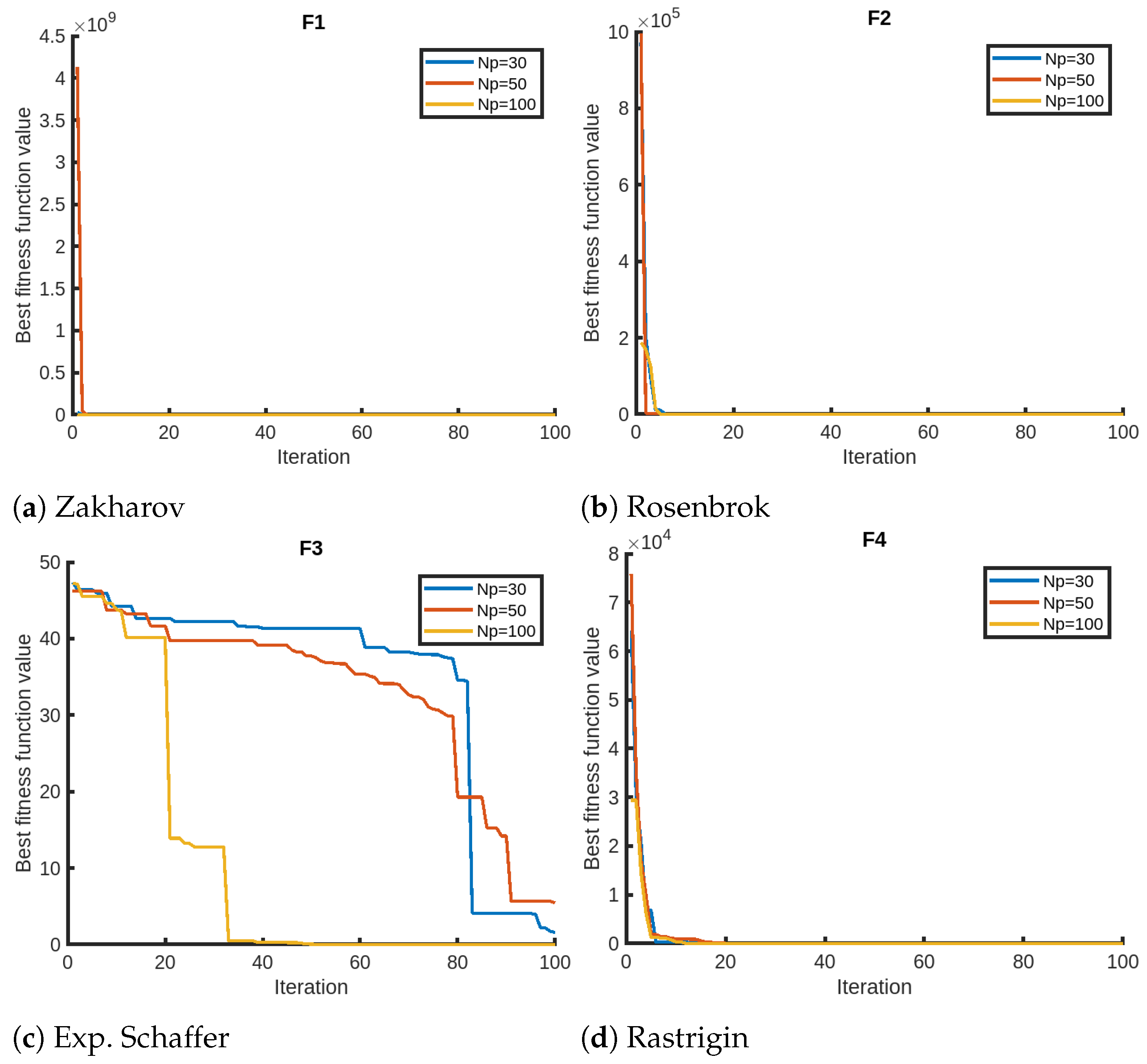
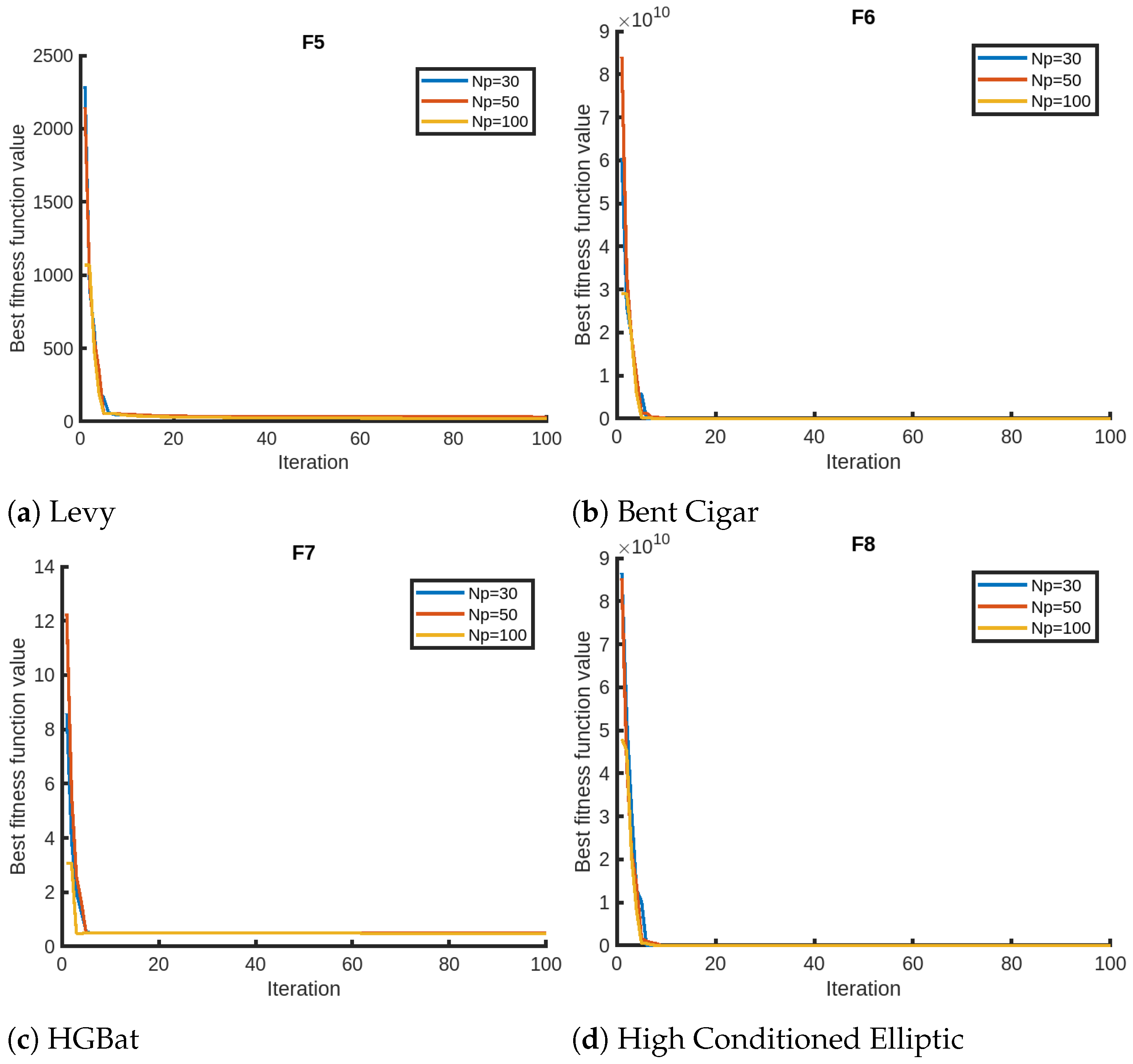
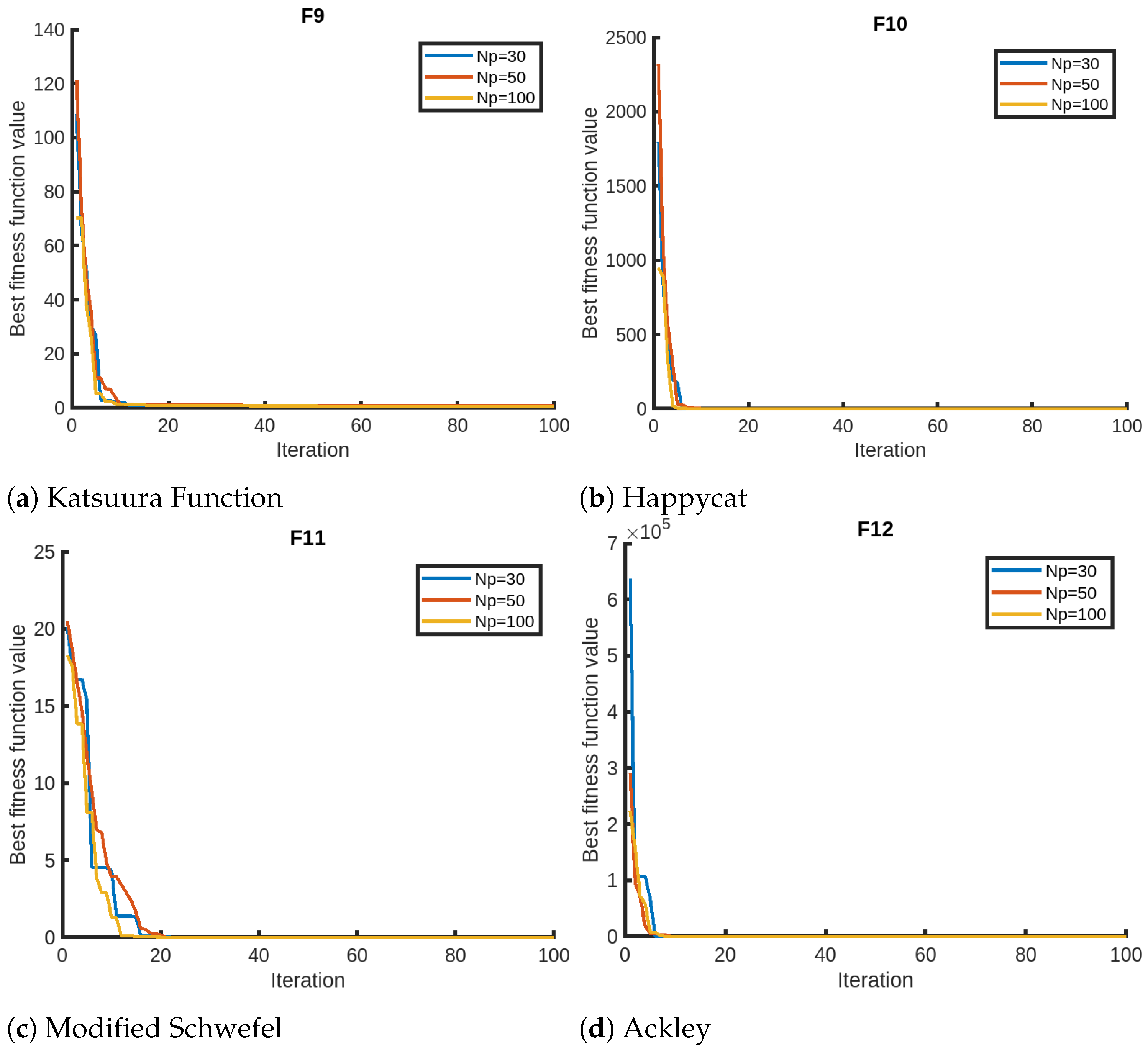
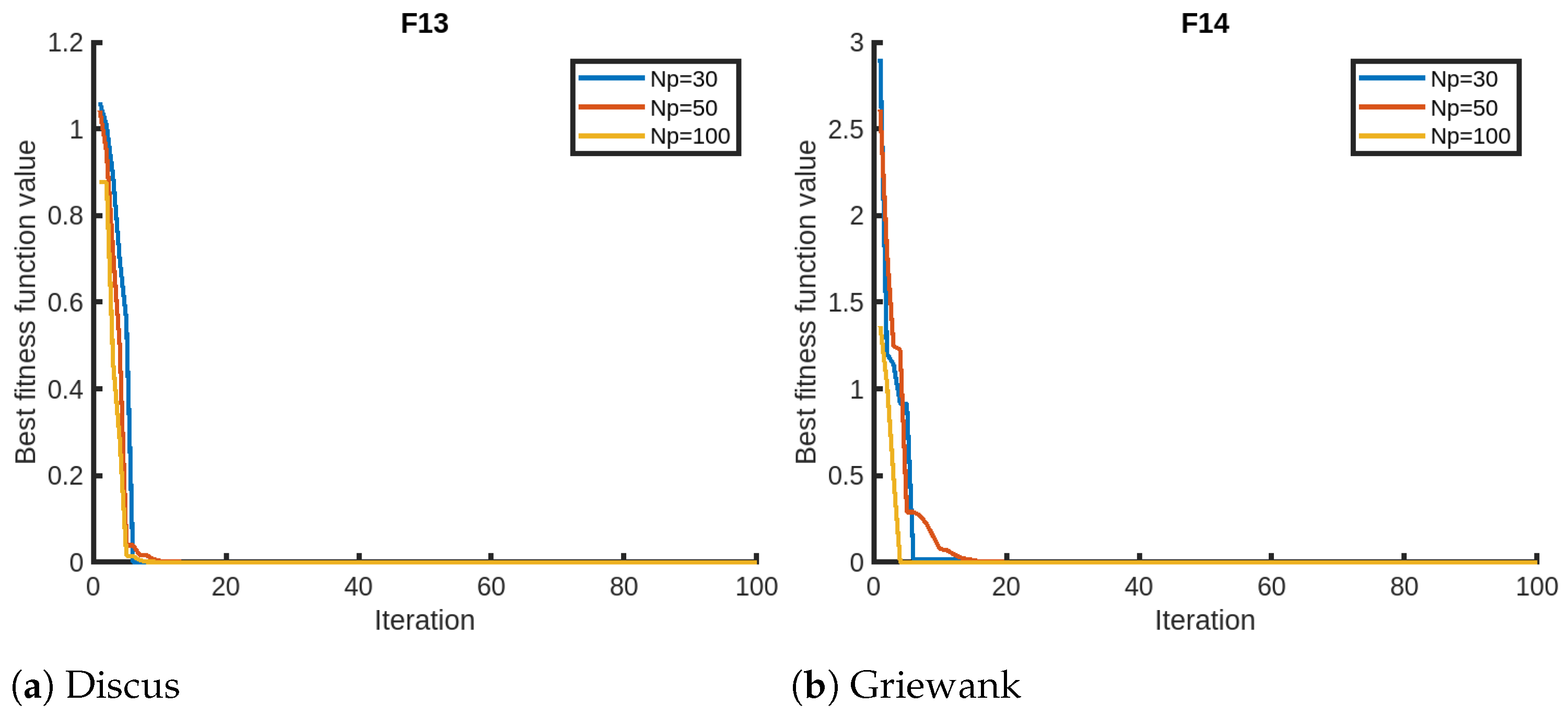
4.3. Sensitivity Analysis

We finally present the sensitivity analysis of QPPA focusing on two parameters, the number of iterations and the number of members in the population, using Setting 1. We evaluate QPPA using $Np=20$, $Np=50$, and $Np=100$. We assess the results for a maximum of 100 iterations for the sensitivity analysis on the maximum number of iterations. We opt for 100 instead of the 1000 iterations due to the faster convergence of QPPA. In Figure 2, we provide visual representations of the sensitivity analysis for the objective functions (F1–F4) that suggest that the population size has a significant impact on the performance of QPPA. Specifically, increasing the population size from $Np=20$ to $Np=50$, and $Np=100$ leads to improved convergence (fitness). We notice that the algorithm takes a longer time than usual for the Exp. Schaffer problem (F3). We notice a similar trend in terms of an improvement in convergence for a larger population size for the rest of the objective functions, as shown in Figure 3, Figure 4 and Figure 5. It is also noticeable that the Ackley function shows a slightly different trend, taking more time than the others. We also note that the fitness score values of HGBat are less than 1, and functions such as Griewank have a smaller range of fitness values. Furthermore, Modified Schwefel has the highest fitness values being reduced, and they are no lower than 3770. These differences are due to the nature of the objective functions according to the properties of their fitness landscapes.

4.4. Further Comparisons

Cooperative coevolution [48] leverages a divide-and-conquer paradigm in evolutionary algorithms to effectively decompose intricate problems into subcomponents (subpopulations) that collaborate and compete among themselves. The collaboration is implemented in terms of fitness evaluations, since the subcomponents feature partial solutions. Cooperative coevolution has been prominent for global optimization problems [49] and neuroevolution [50,51]. There have been a number of extensions of the cooperative coevolution framework [52], including the multi-island competitive cooperative coevolution (MICCC) [53], which used a real-coded genetic algorithm in the subpopulations. Bali and Chandra [54] demonstrated significant improvements in MICC when compared to earlier counterparts, and hence we use it to further compare our results for Setting 2 ($D=100$).

In

Table 8. Optimization results compared to MICCC ($T=15,000$, $D=100$, $N_p=100$).

Function	QPPA	MICCC-6 [54]	MICCC-7 [54]
Ellipsoid	0.00E+00	4.25E−89	0.00E+00
Rosenbrock	5.37E+01	3.47E+01	8.12E+01
Schwefel’s Problem 1.2	0.00E+00	0.00E+00	0.00E+00
Rastrigin	0.00E+00	1.13E−13	0.00E+00

, we present the results of QPPA against MICCC-6 and MICCC-7 across four benchmark functions, where 6 and 7 refer to the number of islands used for competition. Additionally, we include the number of iterations when QPPA achieves the required minimum fitness threshold. We observe the rapid convergence of QPPA in the optimization process. In Figure 6, we present the convergence plots of QPPA for selected objective functions from the 2nd to the 100th iteration. The results of the first iteration, denoting the initial performance, are explicitly reported in the figure captions for a better understanding.

5. Discussion

In summary, QPPA demonstrates superiority over existing algorithms due to the incorporation of quantum principles and predator–prey dynamics. One of the key features is the utilization of a quantum predator mechanism, which enhances the exploration capabilities and enables QPPA to overcome local minima. Instances of this can be seen in Table 3, where QPPA finds the global minima for multiple functions, including Zakharov, Schaffer, Rastrigin, Bent Cigar, High Conditioned Elliptic, Discus, and Griewank. The convergence of QPPA can also be seen in Figure 2, Figure 3, Figure 4 and Figure 5, where it approximately takes 10–20 iterations to converge for simpler problem instances and more iterations for larger problem instances (Figure 2). Moreover, note that in specific cases ($D=100$), as shown in Figure 2b for the Rosenbrock function, we see that there is convergence with a fitness value of less than 100, remaining in a local minimum for a large period of time that exceeds 1000 iterations (Table 6—F2). In Table 8, we note that the results are shown for 15,000 iterations, where QPPA achieves 5.37E+01 for Rosenbrock and MICCC achieves 3.47E+01. However, we note that MICCC uses 1,500,000 function evaluations with a population size of 100, which is equivalent to 150,000 iterations. Hence, we can conclude that QPPA achieves similar convergence to MICCC at a fraction of the time.

Although QPPA performs exceptionally well in general, there are some limitations in certain situations. QPPA in some cases is not able to achieve the same level of performance as algorithms that contain more hyperparameters, which are specifically tuned for the problems. For example, as shown in Table 3, the mayfly optimization algorithm outperforms QPPA in the HGBat, Katsuura, and Modified Schwefel functions, suggesting that QPPA may not be able to adapt to certain problem domains.

In future work, QPPA can be extended by leveraging parallel computing, investigating hybridization strategies, and applying it to the training of machine learning models. Incorporating parallel computing techniques could enhance the efficiency and scalability of QPPA, enabling it to handle larger-scale optimization tasks [55,56]. There are several promising directions for adaptations of QPPA to solve complex problems in the area of discrete parameter optimization. Exploring hybridization strategies for QPPA with other metaheuristic algorithms and for the training of machine learning models could yield enhanced performance, which has been demonstrated for hybrid metaheuristic algorithms in the literature [57,58,59,60]. Finally, machine learning models [61,62] such as deep learning models could enable better performance with the automatic design of network architectures via QPPA-based neuroevolution [63]. Furthermore, QPPA can be implemented using parallel computing and also be applied to large dimensions for the same or similar functions [64], i.e., 1000 dimensions, for it to be compared to large-scale global optimization benchmarks from the literature [65].

Metaheuristic optimization algorithms have drawn criticism in terms of novelty due to an overemphasis on renaming similar processes in nature [66], e.g., there is not a significant difference between the firefly and dragonfly algorithms, and an objective evaluation of their properties remains to be performed. Rajwal et al. [67] reported that more than 500 new metaheuristic algorithms have been introduced in the past few decades. Moreover, many population-based metaheuristics have similar properties, and, over time, many benchmark problems have been defined by researchers, with minimal changes [67]. Hence, it is important to take into account these factors while designing new algorithms, since they could be simply re-implementations of existing algorithms on newer optimization function benchmarks. There has been less focus on parallel implementations and the open sharing of code and resources, which makes the field’s progress challenging. In our study, we try to address some of these shortcomings through a comprehensive study and the open sharing of the code and resources.

6. Conclusions

We demonstrate empirically that QPPA provides a significant contribution to the area of metaheuristic optimization. QPPA features predator–prey interactions and principles of quantum computing, where it emulates the behavior of predators chasing prey. QPPA demonstrated superior performance when compared to eight other algorithms across 14 benchmark optimization functions. Our results demonstrate that QPPA has the ability to reach global minima about 8 - 10 times faster when compared to related algorithms for a wide range of problems. Additionally, it can handle high-dimensional optimization problems and provides better solutions compared to traditional optimization algorithms.

References

1. Hussain, K.; Mohd Salleh, M.N.; Cheng, S.; Shi, Y. Metaheuristic research: A comprehensive survey. Artif. Intell. Rev. 2019, 52, 2191–2233. [Google Scholar] [CrossRef]
2. Silveira, C.L.B.; Tabares, A.; Faria, L.T.; Franco, J.F. Mathematical optimization versus Metaheuristic techniques: A performance comparison for reconfiguration of distribution systems. Electr. Power Syst. Res. 2021, 196, 107272. [Google Scholar] [CrossRef]
3. Halim, A.H.; Ismail, I.; Das, S. Performance assessment of the metaheuristic optimization algorithms: An exhaustive review. Artif. Intell. Rev. 2021, 54, 2323–2409. [Google Scholar] [CrossRef]
4. Chand, S.; Rajesh, K.; Chandra, R. MAP-Elites based Hyper-Heuristic for the Resource Constrained Project Scheduling Problem. arXiv 2022, arXiv:2204.11162. [Google Scholar]
5. Storn, R.; Price, K. Differential evolution-a simple and efficient heuristic for global optimization over continuous spaces. J. Glob. Optim. 1997, 11, 341. [Google Scholar] [CrossRef]
6. Mitchell, M. An Introduction to Genetic Algorithms; MIT Press: Cambridge, MA, USA, 1998. [Google Scholar]
7. Kennedy, J.; Eberhart, R. Particle swarm optimization. In Proceedings of the ICNN’95-International Conference on Neural Networks, Perth, WA, Australia, 27 November–1 December 1995; Volume 4, pp. 1942–1948. [Google Scholar]
8. Dorigo, M.; Birattari, M.; Stutzle, T. Ant colony optimization. IEEE Comput. Intell. Mag. 2006, 1, 28–39. [Google Scholar] [CrossRef]
9. Chandra, R.; Sharma, Y.V. Surrogate-assisted distributed swarm optimisation for computationally expensive geoscientific models. Comput. Geosci. 2023, 27, 939–954. [Google Scholar] [CrossRef]
10. Alba, E.; Luque, G.; Nesmachnow, S. Parallel metaheuristics: Recent advances and new trends. Int. Trans. Oper. Res. 2013, 20, 1–48. [Google Scholar] [CrossRef]
11. Alba, E. Parallel Metaheuristics: A New Class of Algorithms; John Wiley & Sons: Hoboken, NJ, USA, 2005. [Google Scholar]
12. Siddique, N.; Adeli, H. Physics-based search and optimization: Inspirations from nature. Expert Syst. 2016, 33, 607–623. [Google Scholar] [CrossRef]
13. Hashim, F.A.; Houssein, E.H.; Mabrouk, M.S.; Al-Atabany, W.; Mirjalili, S. Henry gas solubility optimization: A novel physics-based algorithm. Future Gener. Comput. Syst. 2019, 101, 646–667. [Google Scholar] [CrossRef]
14. Rashedi, E.; Nezamabadi-Pour, H.; Saryazdi, S. GSA: A gravitational search algorithm. Inf. Sci. 2009, 179, 2232–2248. [Google Scholar] [CrossRef]
15. Tayarani-N, M.H.; Akbarzadeh-T, M. Magnetic optimization algorithms a new synthesis. In Proceedings of the 2008 IEEE Congress on Evolutionary Computation (IEEE World Congress on Computational Intelligence), Hong Kong, China, 1–6 June 2008; pp. 2659–2664. [Google Scholar]
16. Birbil, Ş.İ.; Fang, S.C. An electromagnetism-like mechanism for global optimization. J. Glob. Optim. 2003, 25, 263–282. [Google Scholar] [CrossRef]
17. Fiori, S.; Di Filippo, R. An improved chaotic optimization algorithm applied to a DC electrical motor modeling. Entropy 2017, 19, 665. [Google Scholar] [CrossRef]
18. Steane, A. Quantum computing. Rep. Prog. Phys. 1998, 61, 117. [Google Scholar] [CrossRef]
19. Preskill, J. Quantum computing in the NISQ era and beyond. Quantum 2018, 2, 79. [Google Scholar] [CrossRef]
20. Dunjko, V.; Briegel, H.J. Machine learning & artificial intelligence in the quantum domain: A review of recent progress. Rep. Prog. Phys. 2018, 81, 074001. [Google Scholar]
21. Majot, A.; Yampolskiy, R. Global catastrophic risk and security implications of quantum computers. Futures 2015, 72, 17–26. [Google Scholar] [CrossRef]
22. De Leon, N.P.; Itoh, K.M.; Kim, D.; Mehta, K.K.; Northup, T.E.; Paik, H.; Palmer, B.; Samarth, N.; Sangtawesin, S.; Steuerman, D.W. Materials challenges and opportunities for quantum computing hardware. Science 2021, 372, eabb2823. [Google Scholar] [CrossRef]
23. Khan, A.A.; Ahmad, A.; Waseem, M.; Liang, P.; Fahmideh, M.; Mikkonen, T.; Abrahamsson, P. Software architecture for quantum computing systems—A systematic review. J. Syst. Softw. 2023, 201, 111682. [Google Scholar] [CrossRef]
24. Malossini, A.; Blanzieri, E.; Calarco, T. Quantum genetic optimization. IEEE Trans. Evol. Comput. 2008, 12, 231–241. [Google Scholar] [CrossRef]
25. Yang, S.; Wang, M.; Jiao, L. A quantum particle swarm optimization. In Proceedings of the 2004 Congress on Evolutionary Computation (IEEE Cat. No. 04TH8753), Portland, OR, USA, 19–23 June 2004; Volume 1, pp. 320–324. [Google Scholar]
26. Kaveh, A.; Kamalinejad, M.; Hamedani, K.B.; Arzani, H. Quantum Teaching-Learning-Based Optimization algorithm for sizing optimization of skeletal structures with discrete variables. Structures 2021, 32, 1798–1819. [Google Scholar] [CrossRef]
27. Abd Elaziz, M.; Mohammadi, D.; Oliva, D.; Salimifard, K. Quantum marine predators algorithm for addressing multilevel image segmentation. Appl. Soft Comput. 2021, 110, 107598. [Google Scholar] [CrossRef]
28. Chu, S.C.; Tsai, P.W.; Pan, J.S. Cat swarm optimization. In Proceedings of the PRICAI 2006: Trends in Artificial Intelligence: 9th Pacific Rim International Conference on Artificial Intelligence, Guilin, China, 7–11 August 2006; Proceedings 9. Springer: Berlin/Heidelberg, Germany, 2006; pp. 854–858. [Google Scholar]
29. Kaur, S.; Awasthi, L.K.; Sangal, A.; Dhiman, G. Tunicate Swarm Algorithm: A new bio-inspired based metaheuristic paradigm for global optimization. Eng. Appl. Artif. Intell. 2020, 90, 103541. [Google Scholar] [CrossRef]
30. Teodorović, D. Bee colony optimization (BCO). In Innovations in Swarm Intelligence; Springer: Berlin/Heidelberg, Germany, 2009; pp. 39–60. [Google Scholar]
31. Passino, K.M. Bacterial foraging optimization. In Innovations and Developments of Swarm Intelligence Applications; IGI Global: Hershey, PA, USA, 2012; pp. 219–234. [Google Scholar]
32. Tereshko, V.; Loengarov, A. Collective decision making in honey-bee foraging dynamics. Comput. Inf. Syst. 2005, 9, 1. [Google Scholar]
33. Yazdani, D.; Meybodi, M.R. A novel artificial bee colony algorithm for global optimization. In Proceedings of the 2014 4th International Conference on Computer and Knowledge Engineering (ICCKE), Mashhad, Iran, 29–30 October 2014; pp. 443–448. [Google Scholar]
34. Pian, J.; Wang, G.; Li, B. An improved ABC algorithm based on initial population and neighborhood search. IFAC-PapersOnLine 2018, 51, 251–256. [Google Scholar] [CrossRef]
35. Zervoudakis, K.; Tsafarakis, S. A mayfly optimization algorithm. Comput. Ind. Eng. 2020, 145, 106559. [Google Scholar] [CrossRef]
36. Gao, Z.M.; Zhao, J.; Li, S.R.; Hu, Y.R. The improved mayfly optimization algorithm. J. Phys. Conf. Ser. 2020, 1684, 012077. [Google Scholar] [CrossRef]
37. Johari, N.F.; Zain, A.M.; Noorfa, M.H.; Udin, A. Firefly algorithm for optimization problem. Appl. Mech. Mater. 2013, 421, 512–517. [Google Scholar] [CrossRef]
38. Mirjalili, S. Dragonfly algorithm: A new meta-heuristic optimization technique for solving single-objective, discrete, and multi-objective problems. Neural Comput. Appl. 2016, 27, 1053–1073. [Google Scholar] [CrossRef]
39. Gandomi, A.H.; Yang, X.S.; Alavi, A.H. Cuckoo search algorithm: A metaheuristic approach to solve structural optimization problems. Eng. Comput. 2013, 29, 17–35. [Google Scholar] [CrossRef]
40. Mirjalili, S.Z.; Mirjalili, S.; Saremi, S.; Faris, H.; Aljarah, I. Grasshopper optimization algorithm for multi-objective optimization problems. Appl. Intell. 2018, 48, 805–820. [Google Scholar] [CrossRef]
41. Mirjalili, S.; Lewis, A. The whale optimization algorithm. Adv. Eng. Softw. 2016, 95, 51–67. [Google Scholar] [CrossRef]
42. Mirjalili, S.; Mirjalili, S.M.; Lewis, A. Grey wolf optimizer. Adv. Eng. Softw. 2014, 69, 46–61. [Google Scholar] [CrossRef]
43. Rao, R. Jaya: A simple and new optimization algorithm for solving constrained and unconstrained optimization problems. Int. J. Ind. Eng. Comput. 2016, 7, 19–34. [Google Scholar]
44. Mirjalili, S. SCA: A sine cosine algorithm for solving optimization problems. Knowl.-Based Syst. 2016, 96, 120–133. [Google Scholar] [CrossRef]
45. Berezin, F.A.; Shubin, M. The Schrödinger Equation; Springer Science & Business Media: Berlin/Heidelberg, Germany, 2012; Volume 66. [Google Scholar]
46. Shareef, H.; Ibrahim, A.A.; Mutlag, A.H. Lightning search algorithm. Appl. Soft Comput. 2015, 36, 315–333. [Google Scholar] [CrossRef]
47. Heeren, T.; D’Agostino, R. Robustness of the two independent samples t-test when applied to ordinal scaled data. Stat. Med. 1987, 6, 79–90. [Google Scholar] [CrossRef] [PubMed]
48. Potter, M.A.; De Jong, K.A. A cooperative coevolutionary approach to function optimization. In Proceedings of the International Conference on Parallel Problem Solving from Nature, Jerusalem, Israel, 9–14 October 1994; Springer: Berlin/Heidelberg, Germany, 1994; pp. 249–257. [Google Scholar]
49. Yang, Z.; Tang, K.; Yao, X. Large scale evolutionary optimization using cooperative coevolution. Inf. Sci. 2008, 178, 2985–2999. [Google Scholar] [CrossRef]
50. Potter, M.A.; Jong, K.A.D. Cooperative coevolution: An architecture for evolving coadapted subcomponents. Evol. Comput. 2000, 8, 1–29. [Google Scholar] [CrossRef] [PubMed]
51. Chandra, R.; Ong, Y.S.; Goh, C.K. Co-evolutionary multi-task learning for dynamic time series prediction. Appl. Soft Comput. 2018, 70, 576–589. [Google Scholar] [CrossRef]
52. Ma, X.; Li, X.; Zhang, Q.; Tang, K.; Liang, Z.; Xie, W.; Zhu, Z. A survey on cooperative co-evolutionary algorithms. IEEE Trans. Evol. Comput. 2018, 23, 421–441. [Google Scholar] [CrossRef]
53. Bali, K.K.; Chandra, R. Multi-island competitive cooperative coevolution for real parameter global optimization. In Proceedings of the Neural Information Processing: 22nd International Conference, ICONIP 2015, Istanbul, Turkey, 9–12 November 2015; Proceedings Part III 22. Springer: Berlin/Heidelberg, Germany, 2015; pp. 127–136. [Google Scholar]
54. Bali, K.K.; Chandra, R. Scaling up multi-island competitive cooperative coevolution for real parameter global optimisation. In Proceedings of the AI 2015: Advances in Artificial Intelligence: 28th Australasian Joint Conference, Canberra, ACT, Australia, 30 November–4 December 2015; Proceedings 28. Springer: Berlin/Heidelberg, Germany, 2015; pp. 34–48. [Google Scholar]
55. Alba, E.; Tomassini, M. Parallelism and evolutionary algorithms. IEEE Trans. Evol. Comput. 2002, 6, 443–462. [Google Scholar] [CrossRef]
56. Sudholt, D. Parallel evolutionary algorithms. In Springer Handbook of Computational Intelligence; Springer: Berlin/Heidelberg, Germany, 2015; pp. 929–959. [Google Scholar]
57. Das, S.; Abraham, A.; Konar, A. Particle swarm optimization and differential evolution algorithms: Technical analysis, applications and hybridization perspectives. In Advances of Computational Intelligence in Industrial Systems; Springer: Berlin/Heidelberg, Germany, 2008; pp. 1–38. [Google Scholar]
58. Fister, I.; Mernik, M.; Brest, J. Hybridization of evolutionary algorithms. arXiv 2013, arXiv:1301.0929. [Google Scholar]
59. Grosan, C.; Abraham, A. Hybrid evolutionary algorithms: Methodologies, architectures, and reviews. In Hybrid Evolutionary Algorithms; Springer: Berlin/Heidelberg, Germany, 2007; pp. 1–17. [Google Scholar]
60. Martínez-Estudillo, A.C.; Hervás-Martínez, C.; Martínez-Estudillo, F.J.; García-Pedrajas, N. Hybridization of evolutionary algorithms and local search by means of a clustering method. IEEE Trans. Syst. Man, Cybern. Part B (Cybernetics) 2006, 36, 534–545. [Google Scholar] [CrossRef]
61. Squillero, G.; Tonda, A. Evolutionary algorithms and machine learning: Synergies, Challenges and Opportunities. In Proceedings of the GECCO 2020: Genetic and Evolutionary Computation Conference Companion, Cancún, Mexico, 8–12 July 2020; Association for Computing Machinery, Inc.: New York, NY, USA, 2020; pp. 1190–1205. [Google Scholar]
62. Ibrahim, O.A.S. Evolutionary Algorithms and Machine Learning Techniques for Information Retrieval. Ph.D. Thesis, University of Nottingham, Nottingham, UK, 2017. [Google Scholar]
63. Stanley, K.O.; Clune, J.; Lehman, J.; Miikkulainen, R. Designing neural networks through neuroevolution. Nat. Mach. Intell. 2019, 1, 24–35. [Google Scholar] [CrossRef]
64. Jamil, M.; Yang, X.S. A literature survey of benchmark functions for global optimisation problems. Int. J. Math. Model. Numer. Optim. 2013, 4, 150–194. [Google Scholar] [CrossRef]
65. Mahdavi, S.; Shiri, M.E.; Rahnamayan, S. Metaheuristics in large-scale global continues optimization: A survey. Inf. Sci. 2015, 295, 407–428. [Google Scholar] [CrossRef]
66. Sörensen, K. Metaheuristics—The metaphor exposed. Int. Trans. Oper. Res. 2015, 22, 3–18. [Google Scholar] [CrossRef]
67. Rajwar, K.; Deep, K.; Das, S. An exhaustive review of the metaheuristic algorithms for search and optimization: Taxonomy, applications, and open challenges. Artif. Intell. Rev. 2023, 56, 13187–13257. [Google Scholar] [CrossRef] [PubMed]
Figure 1. QPPA framework highlighting the different stages of the evolution process with predator and prey subpopulations.
Algorithms 17 00033 g001
Figure 2. Sensitivity analyses of QPPA for the population size ( N p ).
Algorithms 17 00033 g002
Figure 3. Sensitivity analyses of QPPA for the population size ( N p ).
Algorithms 17 00033 g003
Figure 4. Sensitivity analyses of QPPA for the population size ( N p ).
Algorithms 17 00033 g004
Figure 5. Sensitivity analyses of QPPA for the population size ( N p ).
Algorithms 17 00033 g005
Figure 6. Convergence graphs of QPPA for selected functions for Setting 2 ( D = 100 ).
Algorithms 17 00033 g006