Specification Mining Based on the Ordering Points to Identify the Clustering Structure Clustering Algorithm and Model Checking

Abstract

Software specifications are of great importance to improve the quality of software. To automatically mine specifications from software systems, some specification mining approaches based on finite-state automatons have been proposed. However, these approaches are inaccurate when dealing with large-scale systems. In order to improve the accuracy of mined specifications, we propose a specification mining approach based on the ordering points to identify the clustering structure clustering algorithm and model checking. In the approach, the neural network model is first used to produce the feature values of states in the traces of the program. Then, according to the feature values, finite-state automatons are generated based on the ordering points to identify the clustering structure clustering algorithm. Further, the finite-state automaton with the highest F-measure is selected. To improve the quality of the finite-state automatons, we refine it based on model checking. The proposed approach was implemented in a tool named MCLSM and experiments, including 13 target classes, were conducted to evaluate its effectiveness. The experimental results show that the average F-measure of finite-state automatons generated by our method reaches 92.19%, which is higher than most related tools.

1. Introduction

With the increasing demand for new functionalities in software, developers often release multiple updates to meet the relevant needs. However, software is frequently released without standard documentation, which leads to the software specification becoming outdated [1]. Moreover, software specification mining requires the expertise of professional developers, since it is a task that requires highly specialized skills to analyze the log documents. Nevertheless, specification mining is necessary as it enables us to identify abnormal system behavior by analyzing system logs. In specification mining, the linear-time temporal logic (LTL) formula and finite-state automaton (FSA) model are generally used to represent software specifications.

Many methods have been proposed to extract system behavior specifications, which allows developers to make informed decisions about the behavior of the system [2,3,4]. Hila Peleg et al. proposed a static technique to mine software specifications directly from the system source code without executing the system [5], but it is not applicable to large-scale systems. Caroline Lemieux et al. proposed an approach to efficiently mine specifications expressed as temporal logic formulas from the execution traces of a system [6]. However, the quality of the mined specifications is not perfect. For instance, if the methods in the input execution traces frequently occur in a particular order or the amount of input traces is too small, the FSAs inferred by k-tails [7] and many other tools are often not generalized and overfitted to the input execution traces. To solve this problem, Tien-Duy et al. proposed deep specification mining (DSM) [8,9], which combines an long short-term memory (LSTM) neural network [10] with the K-means algorithm [11] to mine finite-state automatons (FSAs). LSTM is used in DSM because LSTM is better at learning long-term dependencies and is scalable for long sequences. DSM leverages deep learning techniques to effectively extract the specifications of large-scale systems. It also utilizes clustering algorithms to generate FSAs that more concisely capture the specifications of the systems. However, DSM still faces challenges such as the problem of incorrect merging among states in FSAs generated by clustering feature values and random parameter selection in the clustering process.

To address the above-mentioned issues, we improve DSM by generating FSAs with the ordering points to identify the clustering structure (OPTICS) clustering algorithm [12], and refining the FSAs based on model checking to improve the quality of the FSAs. The proposed specification mining approach can briefly be described as follows:

• DSM is employed to generate the feature values of states in the traces of the program;
• The OPTICS clustering algorithm first generates a reachability plot based on the feature values. Then, the range of the clustering radius is determined according to the reachability plot, and several suitable radii are selected within this range to cluster the feature values to obtain the FSAs;
• A model selection algorithm is used to select the FSA with the highest F-measure from the generated FSAs. Specifically, the F-measure is defined in Section 3.2;
• Texada [6] is employed to generate LTL properties specifying the desired behaviors of the system. Then, model checking of the FSA is performed to verify whether the selected FSA satisfies these properties. If not, we refine the FSA by adding and deleting the corresponding states and transitions in it according to the type of the property which the FSA violates, so that the traces that violate the property are removed from the FSA.

The three main contributions of this paper are as follows:

• We propose a specification mining approach based on the OPTICS clustering algorithm and model checking. Specifically, during the generation of FSAs, we employ the OPTICS clustering algorithm to improve the clustering effect and solve the parameter setting problem so that the parameters can be intuitively set. In addition, we refine the generated FSAs based on model checking to alleviate the problem of incorrect merging among states in FSAs generated by clustering feature values and improve the quality of specifications;
• We implemented our approach in a tool called MCLSM;
• We conducted experiments on 13 target library classes from [8,9,13,14] to evaluate the performance of our tool, and the results show that the average F-measure of the FSAs generated by MCLSM reaches 92.19%, which is 175.85%, 197.67%, 66.95%, 177.17%, 233.41%, 367.49%, and 28.48% higher than that of FSAs generated by the most related tools, i.e., 1-tails [7], 2-tails [7], SEKT 1 [13], SEKT 2 [13], CONTRACTOR++ [13], TEMI [13], and DSM [8,9], respectively.

The remainder of the paper is structured as follows. Section 2 provides the background information. Section 3 introduces the specification mining approach based on the OPTICS clustering algorithm and model checking in detail. We evaluate our approach in Section 4. Section 5 presents the related work and Section 6 concludes the paper.

2. Preliminary

2.1. Model Checking

Model checking is a formal verification technique that determines whether certain properties are satisfied by a system model. In model checking, the system to be verified is modeled as a state transition diagram or finite state automaton. The desired specifications are usually expressed as a set of temporal logic formulas, such as LTL [15] and computing tree logic (CTL) [16]. The basic idea of model checking is to check whether a given specification is satisfied by automatically traversing all possible states of the system. If the system does not satisfy the specification, the model checker generates a counterexample that helps the designer to fix defects in the design.

Here, we focus on model checking of LTL properties. An LTL formula ∅ over a countable set $Pr$ of atomic propositions is inductively defined as follows:

$$\begin{array}{c}\hfill \varphi ::=p|\neg \varphi |{\varphi }_1\wedge {\varphi }_2\left|X\varphi \right|{\varphi }_1\cup {\varphi }_2\end{array}$$

where $p\in Pr$ represents an atomic proposition, ${\varphi }_1$ and ${\varphi }_2$ are all well-formed LTL formulas. For the semantics of these formulas, please refer to [15].

The abbreviations ∨ and → are defined as usual. Some useful derived formulas are given as follows:

$$\begin{array}{c}\hfill F\varphi \stackrel{\mathrm{def}}{=}true\cup \varphi G\varphi \stackrel{\mathrm{def}}{=}\neg F\neg \varphi \end{array}$$

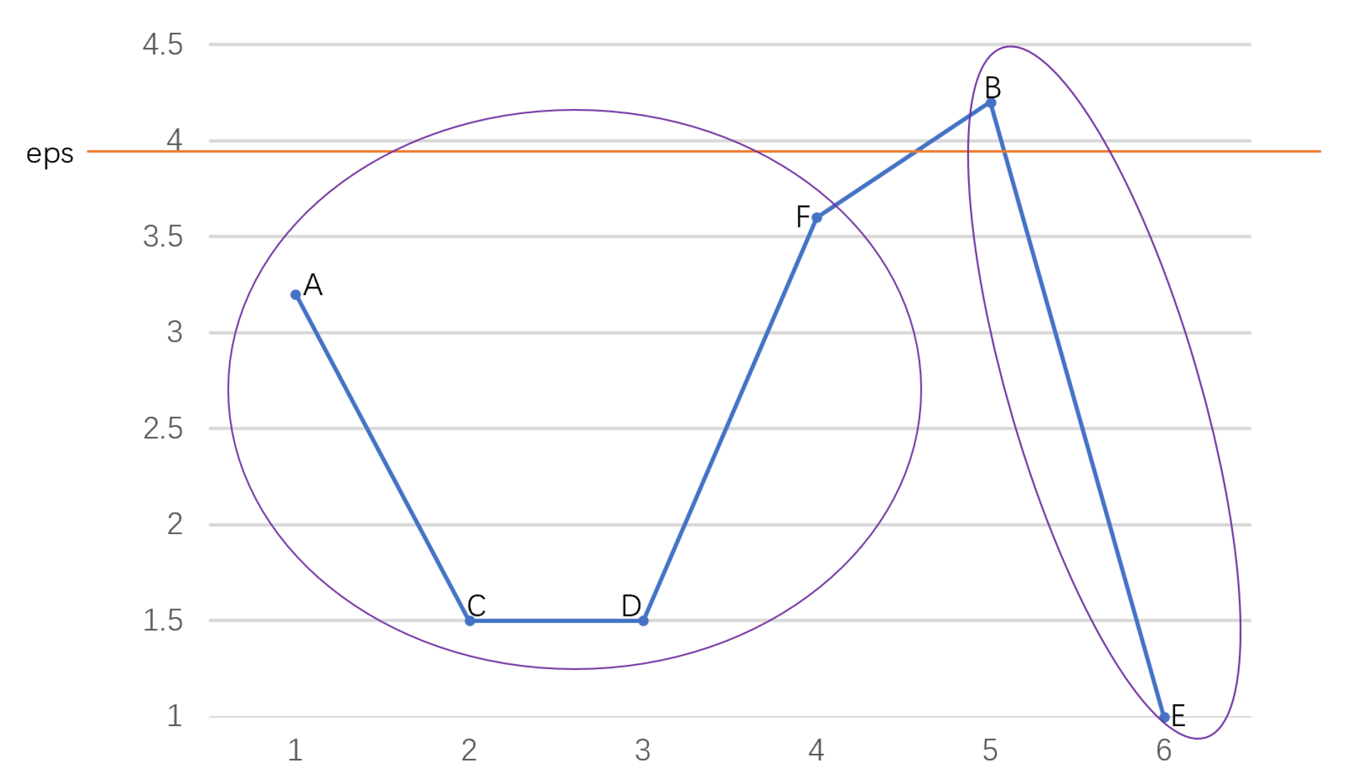
2.2. OPTICS Clustering Algorithm

In the past few decades, the research of clustering algorithms has undergone significant development. Early, K-means [11] clustering algorithms provided a simple and intuitive framework, but their applicability is limited by the data shape and cluster structure. Then, the hierarchical clustering algorithm introduces a hierarchical structure, which provides convenience for understanding the relationship between clusters at different levels. Next, Martin Ester et al. [17] proposed the DBSCAN algorithm, which focuses on density, making clustering more robust for data with an arbitrary shape and density distribution. In recent years, K-means clustering, the Gaussian mixture model (GMM), and mixtures of multivariate clustering algorithms have been applied to the field of chemistry, which has promoted the application of unsupervised learning in other disciplines [18]. With the development of technology, Mantas Lukauskas et al. [19] proposed a density clustering method based on improved inverse formula density estimation. The new method has a good effect when dealing with low dimensional data. In addition, Zhenzhou Wang [20] proposed a clustering method based on morphological operations that worked well on 2D and 3D data.

The OPTICS clustering algorithm creates an augmented ordering of the database representing its density-based clustering structure. Let the object set be O = {$o_1$, $o_2$, …, $o_m$}. Some important definitions associated with the OPTICS clustering algorithm are defined as follows:

• $ϵ$ − $Domain$: For $o_j$ ∈ O, its $ϵ$ − $Domain$ is a subset of O containing objects whose distance from $o_j$ is not greater than $ϵ$. That is, $N_{ϵ}(o_j$) = {$o_i$∈O| distance($o_i$, $o_j$) ≤$ϵ$}. The number of objects in $N_{ϵ}\left(o_j\right)$ is noted as $\mid N_{ϵ}\left(o_j\right)\mid$. Usually, $eps$ is used to represent the clustering radius $ϵ$;
• Core object: for any $o_j$ ∈ O, $o_j$ is a core object if $\mid N_{ϵ}$$\left(o_j\right)\mid$$\ge min\_samples$, where $min\_samples$ is an integer constant;
• Core distance: the minimum radius that makes an object o a core object is called the core distance of o;
• Reachability distance: the reachability distance of an object p with respect to a core object o denoted as $rd(p,o)$ is the maximum value between the actual distance of o to p and the core distance of o.

Let the clustering radius be infinite, i.e., $eps=inf$. OPTICS generates the reachability plot as follows:

• The core object queue $Cq$, ordered queue $Oq$, result queue $Rq$, and reachability distance queue $Rdq$ are initialized to empty;
• All core objects in O are chosen based on $min\_samples$ and $eps$, and then added to $Cq$;
• If there is an element in $Cq$ that has not been processed, jump to 4, and otherwise 8.
• An unprocessed object o is randomly taken out from $Cq$ and placed in $Rq$. Then, it is marked as processed. Further, each object p satisfying $rd(p,o)\le eps$ is selected from $Cq$ and added to $Oq$ in an ascending order of the reachability distance with respect to o;
• If $Oq$ is not empty, jump to 6, and otherwise 3;
• The reachability distance of the first object $p_1$ in $Oq$, with respect to the last object in $Rq$, is stored in $Rdq$. Then, $p_1$ is removed from both $Oq$ and $Cq$, and added into $Rq$;
• Each object whose reachability distance with respect to the last object r in $Rq$ is not greater than $eps$ is selected from $Cq$. Then, these objects are sorted in ascending order of the reachability distance with respect to r and replace the objects in $Oq$. Finally, jump to 5;
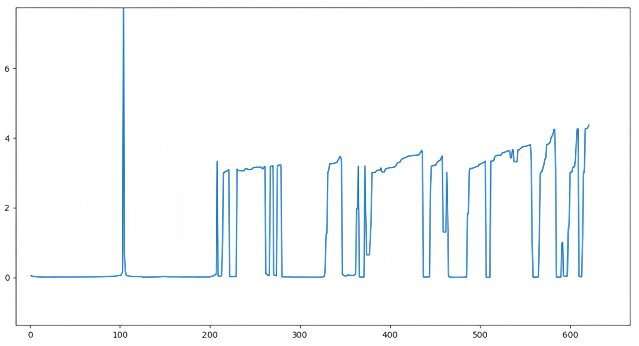
• The reachability plot is plotted based on $Rq$ and $Rdq$.

The OPTICS clustering algorithm [12] is considered more effective than K-means [11] and other clustering algorithms when dealing with high-level data because it can identify changes in density. In terms of clustering parameter selection, OPTICS offers a more reasonable approach compared to clustering algorithms like K-means and DBSCAN [17]. It generates a reachability plot, as depicted in Figure 1, which allows for visual parameter selection. This reduces the impact of randomly setting clustering parameters on the final clustering results. In Figure 1, the horizontal axis represents the sequence of output objects, and the vertical axis stands for the reachability distance of the current object with reference to the previous object, i.e., the reachable distance between object A and object C is 1.5. By setting the value of $eps$ to 3.9, all the objects can be effectively divided into two clusters: {A,C,D,F} and {B,E}.

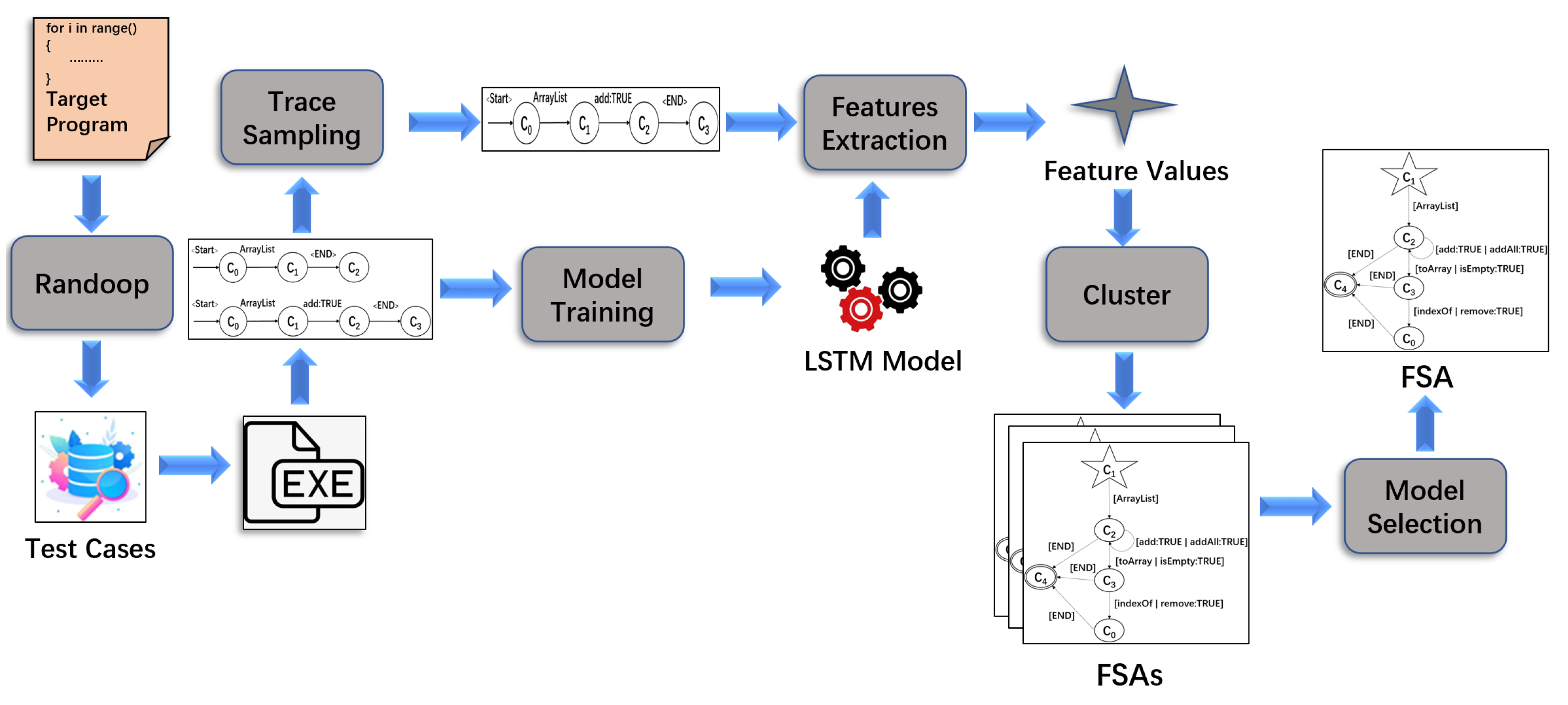
2.3. DSM

DSM is a state-of-the-art specification mining tool [8,9], which applies deep learning to specification mining in order to improve the accuracy of the mined automata. However, it also experiences the merging of errors problem between states of the final obtained automata. DSM involves six processes: test case generation and trace collection, model training, trace sampling, feature extraction, clustering, and model selection. As shown in Figure 2, the skeleton of the approach is briefly given as follows:

• DSM uses Randoop [21] to generate a large number of test cases. Then, it executes the target program with these cases and stores the traces (the methods calls) of the program in a trace set;
• The LSTM model is trained by all execution traces;
• In order to improve the efficiency of specification mining, a subset $STr$ of traces that can cover all adjacent method pairs of execution traces is extracted;
• Two types of features, i.e., $F_m^i$ and $P_m^i$, are extracted in each state $S_i$ based on the subset of traces and the LSTM model, where $F_m^i$ captures information of previously invoked methods before $S_i$, and $P_m^i$ captures information about methods immediately after state $S_i$ using the LSTM model. For instance, suppose that all methods that appear in the program are in a set $M=\{m_1,m_2,\dots ,m_n\}$ and a trace is $tr$ = $\langle m_{x1}$, …, $m_{xk}$, …, $m_{xl}\rangle$, where $m_{xi}$ ($1\le i\le l$ and $m_{xi}\in M$) in $tr$ is the invoked method at state $S_i$. At state $S_k$, methods from $m_{x1}$ to $m_{xk}$ in $tr$ are invoked. Thus, $F_{m_{xi}}^k=1$ ($1\le i\le k$) and for other methods $m_j$ in M, $F_{m_j}^k=0$. All feature values of all states in all traces belonging to the subset $STr$ are stored in a set O = {$o_1$=$\langle B_1$, $A_1\rangle$, …, $o_l$ = $\langle B_h$, $A_h\rangle$}, where h is the number of states in all traces and for each $1\le y\le h$, $B_y$ = $\langle F_{m_1}^y$, …, $F_{m_n}^y\rangle$, and $A_y$ = $\langle P_{m_1}^y$, …, $P_{m_n}^y\rangle$;
• The K-means [11] and hierarchical clustering algorithms are used to cluster the feature values and generate FSAs. An FSA can be represented as a five-tuple D = (Q, $\Sigma$, $\delta$, $q_0$, F), where Q is a finite set of states, $\Sigma$ is a table of input characters, $\delta$ is a transition function mapping Q × $\Sigma$ to Q, $q_0$ ∈ Q is the initial state, and F ⊂ Q is the set of acceptable states;
• The FSA with the highest F-measure is selected from the generated FSAs.

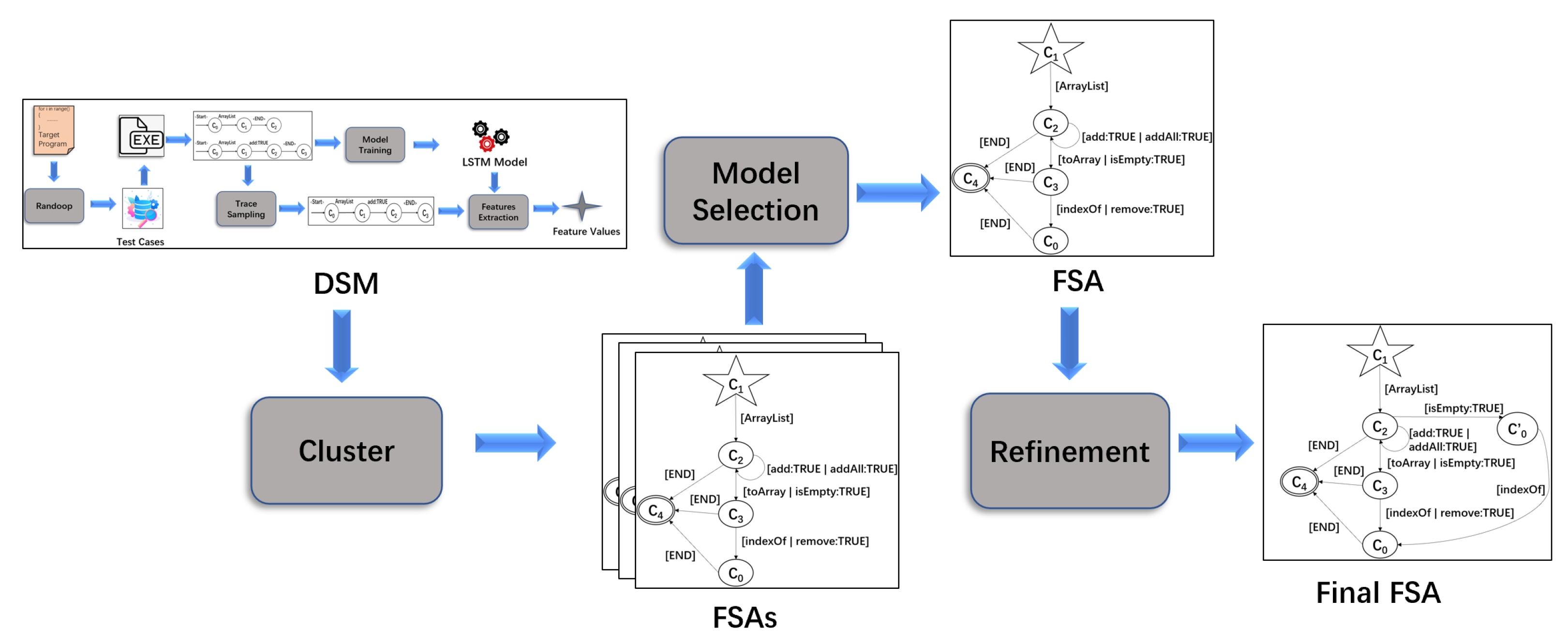
3. Specification Mining Based on the OPTICS Clustering Algorithm and Model Checking

Our approach involves three key processes: clustering, model selection, and refinement. As shown in Figure 3, the skeleton of the approach is briefly given as follows:

• We cluster feature values obtained by DSM based on $eps$ in the reachability plot, which is drawn according to the OPTICS clustering algorithm [12];
• The FSAs with the highest F-measure are selected during the model selection;
• We perform model checking on the selected FSAs and refine the FSAs based on the verification result to obtain the final FSAs.

3.1. Clustering

In order to create an automaton that captures the specification of the target library classes, the feature values in set O generated by DSM are clustered to generate FSAs, where O = {$o_1=\langle B_1,A_1\rangle ,\dots ,o_h=\langle B_h,A_h\rangle$} as defined in Section 2.2.

To do that, some variables used in the clustering algorithm are defined as follows:

• $Cq$, $Rq$, and $eps$ are defined as in Section 2.2;
• $Kq$ is used to store objects of the same class as a given object;
• K is used to mark the category to which the current objects belong;
• The map $Labels$ is used to map the category K to the corresponding core objects at one clustering;
• $All\_labels$ is used to store $Labels$ after each clustering;
• The variable $num$ is used to control the increment of $eps$ at each clustering;
• $Plot$ represents the reachability plot generated by the OPTICS clustering algorithm.

In order to alleviate the influence of clustering parameters on the clustering results, we first use the OPTICS clustering algorithm shown in Section 2.2 to generate the reachability plot, and then determine the range of $eps$ and the value of $num$ based on the plot. Further, we cluster objects in O according to $eps$ and $num$ to generate FSAs. Algorithm 1 shows the clustering process. It takes the feature values in O extracted by DSM as the input, and outputs a set $All\_labels$ storing well-classified feature values after multiple clustering. In the algorithm, we first initialize $Cq$, $Kq$, $Rq$, $Labels$, and $All\_labels$ to ∅, and $eps$ to $inf$ (Line 1). Then, the reachability plot $Plot$ is generated based on OPTICS clustering algorithm $OPTICS\_RPlot\left(O\right)$, the details of which are shown in Section 2.2 (Line 2). The purpose of generating $Plot$ is to observe the shape and trend in order to determine the appropriate range $[a,b]$ of $eps$ and the increment value $num$ of $eps$ for each time of clustering (Line 3). In order to obtain $All\_labels$, which is required to generate FSAs, we cluster the feature values in O with $eps$ ranging from a to b (Lines 4–22). For each clustering time, we first find all core objects needed for clustering from O and add them to $Cq$ (Line 6). Then, we cluster the core objects in $Cq$ to obtain $Labels$. The following is the process of how we generate $Labels$. We first find objects whose distances to $Cq\left[0\right]$ are not greater than $eps$ in $Cq$ (except $Cq\left[0\right]$), and add them to $Kq$, which stores objects of the same category as $Cq\left[0\right]$. Then, we remove $Cq\left[0\right]$ from $Cq$ and put it in $Rq$. The distance is the Euclidean distance between two feature values, i.e., two objects (Lines 9–10). Further, we find the core objects in $Cq$ that belong to the same class as each object in $Kq$, and add these objects to $Kq$ until all objects in $Kq$ are processed. Each time the objects added to $Kq$ should be deleted from $Cq$ to avoid duplication, and the objects that have been processed in $Kq$ should also be removed and added to $Rq$ (Lines 11–14). When $Kq$ is empty, we mark the objects in $Rq$ as class K and set $Rq$ to empty in order to continue classifying the remaining objects in $Cq$ (Lines 15–16). When $Cq$ is empty, a clustering of objects in $Cq$ is completed. We add $Labels$ to $All\_labels$ and set $Labels$ to empty for generating the next $Labels$ (Lines 19–21). Finally, we construct FSAs based on $All\_lables$ according to the method in [9].

Figure 4 shows an FSA generated based on the OPTICS clustering algorithm. In the FSA, the start state is $q_0$ = $C_1$ and the set of acceptable states is F = $\left\{C_4\right\}$. The input character table $\Sigma$ is a collection of methods, Q is a collection of all states, and each transition between method and its connected states makes up the transition function $\delta$.

Algorithm 1: Clustering Process
	Input: O
	Output: $All\_labels$
1	Initialize: $Cq$, $Kq$, $Rq$, $Labels$, $All\_labels$ = ∅, $eps=inf$;
2	$Plot$ = $OPTICS\_RPlot\left(O\right)$;
3	Determine the range $[a,b]$ of $eps$ and the value of $num$ according to $Plot$;
4	$eps=a$;
5	while $eps\le b$ do
6		$Cq$← Find all core objects in O based on $eps$ and $min\_samples$;
7		$K=0$;
8		while $Cq$ ≠ ∅ do
9			$Rq$← Take out $Cq\left[0\right]$ from $Cq$;
10			$Kq$← Take out all objects o satisfying $distance(o,Rq[n-1\left]\right)\le eps$ from $Cq$;
			//  $\phantom{(}$n represents the number of objects in $Rq$
11			while $Kq$ ≠ ∅ do
12				$Kq$← Take out all objects $o^{\prime }$ satisfying $distance(o^{\prime },Kq\left[0\right])\le eps$ from $Cq$;
13				$Rq$← Take $Kq\left[0\right]$ out of $Kq$;
14			end
15			$Labels$← Grouping objects in $Rq$ into K category;
16			$Rq$ = ∅;
17			K = K + 1;
18		end
19		$All\_labels$←$Labels$;
20		$Labels$ = ∅;
21		$eps$ = $eps+num$;
22	end
23	return $All\_labels$;

3.2. Model Selection

DSM [8,9] often chooses the best FSA by predicting the $Precision$ and $Recall$ of all generated FSAs. Here, we define $Precision$ and $Recall$ as follows:

$$Precision\left(D\right)=\frac{|M{P}_{TR}\cap fsa\_pairs\left(D\right)|}{|fsa\_pairs(D\left)\right|}$$

(1)

where D is the FSA to be evaluated, $M{P}_{TR}$ represents all method pairs appearing in the input trace set $TR$, and $fsa\_pairs\left(D\right)$ represents the method pairs appearing in D. Note that we call a method pair (x, y) that appears in D if x and y are labeled at two adjacent edges in D, respectively. In fact, we should consider the traces in $TR$ as positive samples and the traces in D as classified into positive samples. However, the number of traces in D usually cannot be calculated. Thus, we consider the method pairs in $TR$ as positive samples and the method pairs in D as classified into positive samples. In Formula (1), |$fsa\_pairs\left(D\right)$| represents the data that are classified as positive, and |$M{P}_{TR}$ ∩ $fsa\_pairs\left(D\right)$| represents the data that are actually positive in the classification.

$$Recall=\frac{|accepted\_trace|}{\left|TR\right|}$$

(2)

where |$accepted\_traces$| represents the number of traces in the trace set that the generated FSA can accept, and |$TR$| represents the number of all execution traces. Using just one of $Precision$ or $Recall$ to evaluate an FSA cannot comprehensively evaluate the advantages and disadvantages of the FSA. A higher $Precision$ means an FSA accepts fewer traces that should not be accepted, while a higher $Recall$ means an FSA accepts more traces that should be accepted. Thus, we combine $Precision$ and $Recall$ to obtain the F-measure (Formula (3)) as the actual scoring criteria.

$$F-measure=2\times \frac{Precision\times Recall}{Precision+Recall}$$

(3)

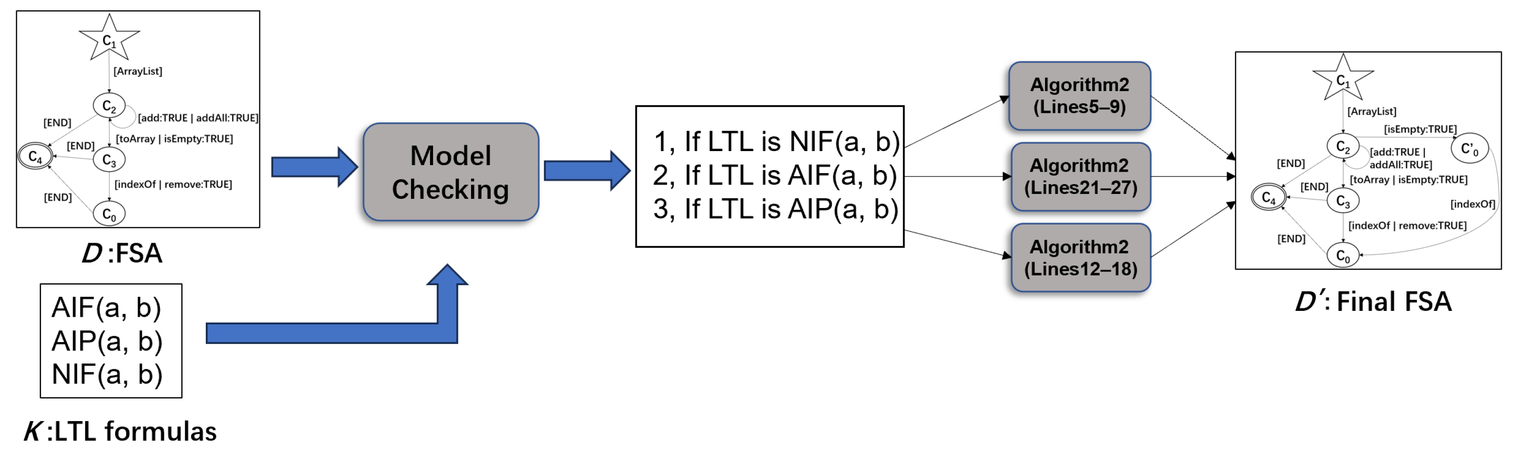
3.3. FSA Refinement Based on Model Checking

The FSAs generated in Section 3.1 are prone to incorrect paths in the model due to erroneous merging among states.

To mitigate this issue, we refine the FSAs based on model checking. Specifically, we explore the FSA and check if it satisfies the LTL formulas. When a violation is detected, we refine the automaton to eliminate the violation and improve the precision of the FSA. We repeat this process until there is no violation or the number of times for the refinement reaches a threshold value T.

In order to use the partial specification of the software (LTL formulas) to guide the refinement of the overall specification of the software (FSA), we input the traces generated in DSM [8,9], property templates, and confidence thresholds into Texada [6] to generate the following three forms of LTL formulas, which were shown to specify the temporal properties of automata by Beschastnikh et al. [22].

• $AIF(a,b)$: an occurrence of event a must be immediately followed by event b, i.e., G (a→Xb);
• $AIP(a,b)$: an occurrence of event a must be immediately preceded by event b, i.e., F$\left(a\right)$→ (¬a∪ (b∧Xa));
• $NIF(a,b)$: an occurrence of event a is never immediately followed by event b, i.e., G (a→X (¬b)).

The variables used in the refinement process are defined as follows:

• D and $D^{\prime }$ represent the FSAs before and after refinement, respectively;
• K is a set of LTL formulas generated by Texada;
• $Trans$ is a set of tuples $\langle SM,q_2,m_2,q_3,MS\rangle$, where $SM$ is a set of tuples $\langle q_1,m_1\rangle$, $MS$ is a set of tuples $\langle m_3,q_4\rangle$, $q_1$, $q_2$, $q_3$, and $q_4$ are states, and $m_1$, $m_2$, $m_3$, and $m_4$ are methods;
• $C_i^{\prime }(1\le i\le num)$ represents newly added states in the FSA.

Algorithm 2 and Figure 5 show the refinement process based on model checking in detail, where the initial FSA D and a set K of LTL formulas are taken as the input. In the process, $num$ and $times$ are initialized to 0 and $D^{\prime }$ is initialized to D (Line 1). We then verify whether the number of times for refinement reaches the threshold value, and whether there exists a property violated by the FSA, i.e., whether the software behavior described by FSA does not match that described by the LTL formula (Line 2). If so, $FindErrTr$ returns the set $Trans$ of error segments in the FSA according to the type of violated property as follows:

Algorithm 2: Refinement Process
	Input: D = (Q, $\Sigma$, $\delta$, $q_0$, F), K = {$K_1$, …, $K_t$}
	Output: $D^{\prime }$= ($Q^{\prime }$, $\Sigma$, ${\delta }^{\prime }$, $q_0$, F)
1	Initialize: $num=0$, $times=0$, $D^{\prime }=D$;
2	while $times++<T$ and there exists a property $K_j\in K$ violated by $D^{\prime }$ do
3		$Trans=FindErrTr(K_j,D^{\prime })$;
4		for each $\langle SM,q_2,m_2,q_3,MS\rangle \in Trans$ do
5			if $K_j$ is $NIF(a,b)$ then
6				Delete ${\delta }^{\prime }$ ($q_2$, $m_2$) = $q_3$;
7				$Q^{\prime }=Q^{\prime }\cup \{C_{num}^{\prime }$};
8				Add transition rules to ${\delta }^{\prime }$: ${\delta }^{\prime }$ ($q_2$, $m_2$) = $C_{num}^{\prime }$ and ${\delta }^{\prime }$ ($C_{num}^{\prime }$, $m_3$) = $q4$ for
				each $\langle m_3,q_4\rangle \in MS$;
9				$num$ = $num$ + 1;
10			end
11			if $K_j$ is $AIP(a,b)$ then
12				Delete ${\delta }^{\prime }$ ($q_2$, $m_2$) = $q_3$;
13				$Q^{\prime }=Q^{\prime }\cup \left\{C_{num}^{\prime }\right\}$;
14				Add transition rules to ${\delta }^{\prime }$: ${\delta }^{\prime }$ ($q_1$, $m_1$) = $C_{num}^{\prime }$ for each $\langle q_1,m_1\rangle \in SM$;
15				$num$ = $num$ + 1;
16				$Q^{\prime }=Q^{\prime }\cup \left\{C_{num}^{\prime }\right\}$;
17				Add transition rules to ${\delta }^{\prime }$: ${\delta }^{\prime }$ ($C_{num-1}^{\prime }$, a) = $C_{num}^{\prime }$ and ${\delta }^{\prime }$ ($C_{num}^{\prime }$, $m_2$) = $q_3$;
18				$num$ = $num$ + 1;
19			end
20			if $K_j$ is $AIF(a,b)$ then
21				Delete ${\delta }^{\prime }$ ($q_2$, $m_2$) = $q_3$;
22				$Q^{\prime }=Q^{\prime }\cup \left\{C_{num}^{\prime }\right\}$;
23				Add a transition rule to ${\delta }^{\prime }$: ${\delta }^{\prime }$ ($q_2$, $m_2$) = $C_{num}^{\prime }$;
24				$num$ = $num$ + 1;
25				$Q^{\prime }=Q^{\prime }\cup \{C_{num}^{\prime }$};
26				Add transition rules to ${\delta }^{\prime }$: ${\delta }^{\prime }$ ($C_{num-1}^{\prime }$, b) = $C_{num}^{\prime }$ and ${\delta }^{\prime }$ ($C_{num}^{\prime }$, $m_3$) = $q_4$
				for each $\langle m_3,q_4\rangle \in MS$;
27				$num$ = $num$ + 1;
28			end
29		end
30		$D^{\prime }$ = ($Q^{\prime }$, $\Sigma$, ${\delta }^{\prime }$, $q_0$, F);
31	end

• If the violated property is $NIF(a,b)$, it returns all segments $\langle SM,q_2,m_2,q_3,$$MS\rangle$ that satisfy $m_2=a$, ${\delta }^{\prime }(q_2,a)=q_3$, $SM$ containing all tuples $\langle q_1,m_1\rangle$ satisfying ${\delta }^{\prime }(q_1,m_1)=q_2$, $MS$ containing all tuples $\langle m_3,q_4\rangle$ satisfying ${\delta }^{\prime }(q_3,$$m_3)=q_4$, and there is $\langle m_3^{\prime },q_4^{\prime }\rangle \in MS$ satisfying $m_3^{\prime }=b$;
• If the violated property is $AIP(a,b)$, it returns all segments $\langle SM,q_2,m_2,q_3,$$MS\rangle$ that satisfy $m_2=b$, ${\delta }^{\prime }(q_2,b)=q_3$, $MS$ containing all tuples $\langle m_3,q_4\rangle$ satisfying ${\delta }^{\prime }(q_3,$$m_3)=q_4$, $SM$ containing all tuples $\langle q_1,m_1\rangle$ satisfying ${\delta }^{\prime }(q_1,m_1)=q_2$, and for each $\langle q_1,m_1\rangle \in SM$, $m_1\ne a$;
• If the violated property is $AIF(a,b)$, it returns all segments $\langle SM,q_2,m_2,q_3,$$MS\rangle$ that satisfy $m_2=a$, ${\delta }^{\prime }(q_2,a)=q_3$, $SM$ containing all tuples $\langle q_1,m_1\rangle$ satisfying ${\delta }^{\prime }(q_1,m_1)=q_2$, $MS$ containing all tuples $\langle m_3,q_4\rangle$ satisfying ${\delta }^{\prime }(q_3,$$m_3)=q_4$, and for each $\langle m_3,q_4\rangle \in MS$, $m_3\ne b$.

Further, we refine the FSA with different refinement rules depending on the type of formula that the error segment $\langle SM,q_2,m_2,q_3,MS\rangle$ violates as follows:

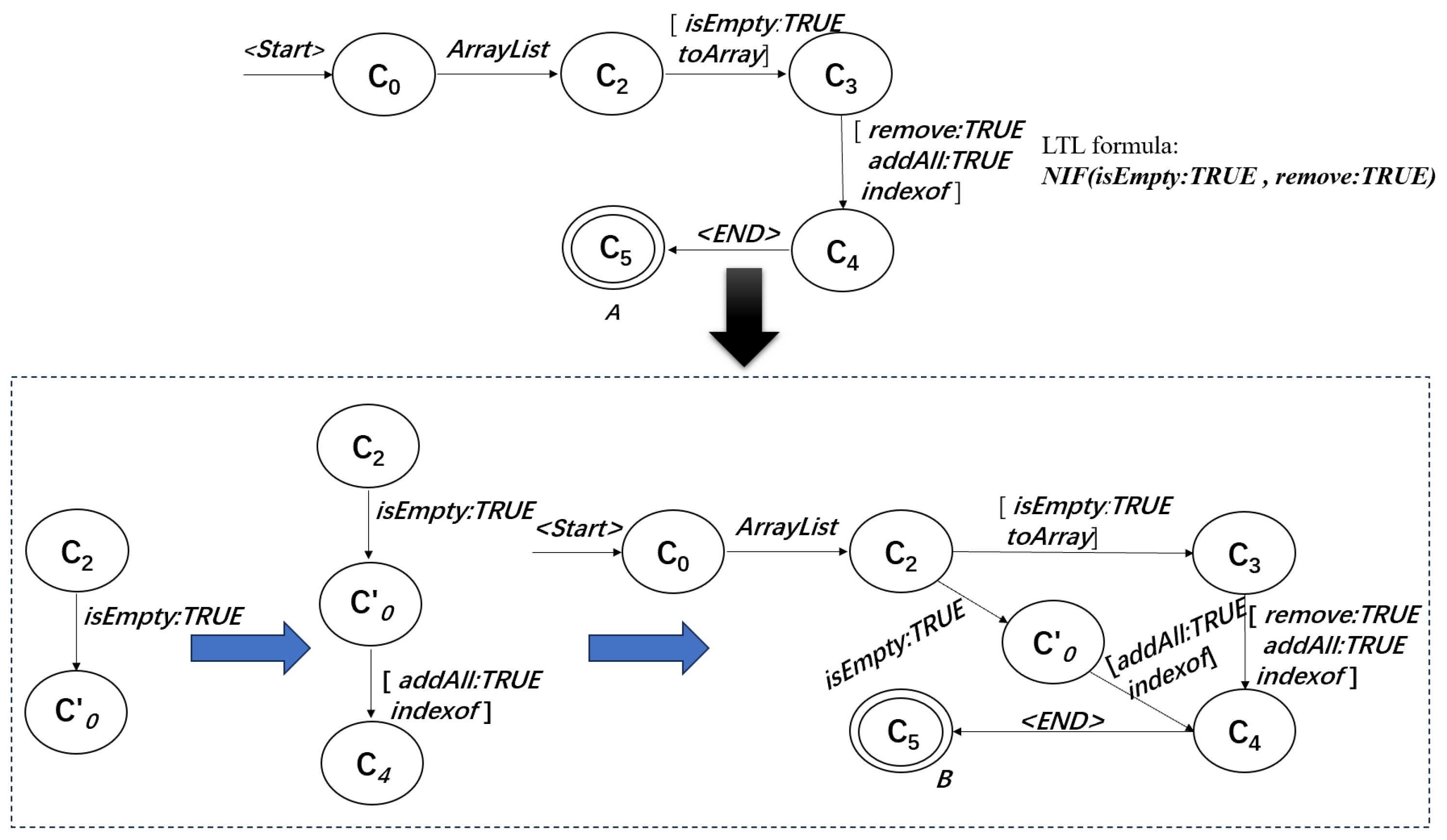
• If it violates $NIF(a,b)$, $m_2=a$, we first delete the transition rule from state $q_2$ to state $q_3$ using method a, so that the traces violating $NIF(a,b)$ are removed (Line 6). Then, in order to prevent traces that do not violate $NIF(a,b)$ from being deleted, we add a state $C_{num}^{\prime }$ and some transition rules. First, we add a transition rule from state $q_2$ to state $C_{num}^{\prime }$ using method a. Next, we add transition rules from $C_{num}^{\prime }$ to each $q_4$ in $MS$ using the corresponding method (except b) in $MS$ (Lines 7–8);
• If it violates $AIP(a,b)$, $m_2=b$, we first delete the transition rule from state $q_2$ to state $q_3$ using method b, so that the traces violating $AIP(a,b)$ are removed (Line 12). Then, in order to increase the precision of the automaton, we add a state $C_{num}^{\prime }$ and transition rules from each state $q_1$ in $SM$ to $C_{num}^{\prime }$ using the corresponding method in $SM$. Next, we update the state subscript $num$ and create another new state $C_{num}^{\prime }$. Further, we add a transition rule from state $C_{num-1}^{\prime }$ to state $C_{num}^{\prime }$ using method a and a transition rule from state $C_{num}^{\prime }$ to state $q_3$ using method b (Lines 13–17);
• If it violates $AIF(a,b)$, $m_2=a$, we first delete the transition rule from state $q_2$ to state $q_3$ using method a, so that the traces violating $NIF(a,b)$ are removed (Line 21). Then, in order to increase the precision of the automaton, we add a state $C_{num}^{\prime }$ and some transition rules. First, we add a transition rule from state $q_2$ to state $C_{num}^{\prime }$ using method a. Next, we update the state subscript $num$ and create a new state $C_{num}^{\prime }$. We then add a transition rule from $C_{num-1}^{\prime }$ to $C_{num}^{\prime }$ using method b and transition rules from $C_{num}^{\prime }$ to each state $q_4$ in $MS$ using the corresponding method in $MS$ (Lines 23–26).

After performing a round of refinement, we generate a new FSA $D^{\prime }$, and the next round of refinement is performed on the basis of $D^{\prime }$ (Line 30).

The example in Figure 6 shows the refinement process for an FSA that violates $NIF(isEmpty:TRUE,remove:TRUE)$. First of all, we use model checking with the LTL formula to find an error segment $\langle SM=\left\{\langle C_0,ArrayList\rangle \right\},q_2=C_2,m_2=isEmpty:True,q_3=C_3,MS=\{\langle remove:TRUE,C_4\rangle ,\langle add:All:TRUE,C_4\rangle ,\langle indexof,C_4\rangle \}\rangle$ violating $NIF(isEmpty:TRUE,remove:TRUE)$. Next, we delete the transition rule from $C_2$ to $C_3$ through $isEmpty:TRUE$, so that the trace that violates $NIF(isEmpty:TRUE,remove:TRUE)$ is removed. Further, in order to prevent traces that do not violate $NIF(isEmpty:TRUE,remove:TRUE)$ from being deleted, we add a transition rule from $C_2$ to $C_0^{\prime }$ through $isEmpty:TRUE$ and transition rules from $C_0^{\prime }$ to $C_4$ through $addAll:TRUE$ and $indexof$. After the above operation, we have refined model A, which contained errors, into model B, which is error-free.

4. Empirical Evaluation

We implemented the proposed approach in a tool named MCLSM and evaluated our approach to answer the following question: How effective is MCLSM compared with the existing specification mining tools?

4.1. Dataset

In the experiment, we used all 13 target library classes from [8,9,13,14] as the benchmark to evaluate MCLSM.

In this benchmark, ArrayList serves as the implementation of a variable-size array of list interfaces, while LinkedList is primarily employed for creating linked list data structures. HashSet, implementing the set interface, ensures the absence of duplicate elements and does not guarantee the order of elements. HashMap, functioning as a Hashtable, facilitates key-value mapping with rapid access speeds. Hashtable, originating from the original java.util, is a concrete implementation of a dictionary. The Signature class in Java is utilized to provide a digital signature algorithm for applications, while the Socket class offers a comprehensive set of network communication methods and properties. ZipOutputStream allows direct content writing to the zip package. The StringTokenizer class implements both the Iterator and Enumeration interfaces. These nine target class libraries are integral components of the Java Development Kit. Additionally, four other class libraries are used, namely, StackAr from the Daikon project, NFST (NumberFormatStringTokenizer) and ToHTMLStream from Apache, and SMTPProtocol from Columba.ristretto.

Table 1. Target library classes.

Target Library Class1	M	Generated Test Case	Recorded Method Calls
ArrayList	18	42,865	22,996
LinKedList	7	13,731	4847
HashSet	8	23,181	257,428
HashMap	11	53,396	67,942
Hashtable	8	79,403	89,811
Signature	5	79,096	205,386
Socket	21	80,035	130,876
ZipOutputStream	5	162,971	43,626
SringTokenizer	5	148,649	336,924
StackAr	7	549,648	132,826
NFST	5	158,998	95,149
ToHTMLStream	17	103,562	278,631
SMTPProtocol	15	57,281	136,271

shows the information of these classes. The column “Target Library Class” displays the names of the target classes. The column “M” lists the number of class methods analyzed in the target classes. The column “Generated Test Cases” is the number of test cases generated by Randoop, and the column “Recorded Method Calls” gives the number of method calls recorded in all execution traces of the target classes. The data in Table 1 consist of 13 target classes, which are both complex and simple; thus, we chose to use these data to evaluate the effectiveness of our method on different sizes of data.

4.2. Experience Setting

The experiments were carried out on a 64-bit Ubuntu 18.04 LTS with a 3.20 GHz Intel(R) Core(TM) i5-10505 processor and 16 GB memory. MCLSM uses the OPTICS clustering algorithm to cluster feature values. During the clustering process, we set $min\_samples$ to 5, and selected the range of $eps$ according to the reachability plot. In the clustering process, $eps$ represents the radius of the cluster and is used to determine whether one point can reach another. By adjusting the size of the $eps$ value, we can change the shape of the cluster. Smaller $eps$ may result in the formation of more and smaller clusters, while larger $eps$ may combine more points into one cluster. Therefore, it is very important to select the appropriate $eps$ in datasets with uneven densities. We determined the range of $eps$ using the reachability plot and adjusted the $eps$ in this range to achieve the best clustering effect. In a reachability plot, the boundaries of a cluster usually correspond to points with large variation in reachable distance, that is, high or low points. First, we set a threshold. Then, we found all the high and low points in the reachability plot and removed points larger than the threshold. Next, we determined the range of $eps$ using the maximum and minimum values of these points. Finally, we selected the appropriate step size to cluster within the defined range and obtained the most suitable $eps$ value for the current data according to the clustering effect. For example, Figure 7 shows the reachability plot generated for the ArrayList class, where the horizontal axis represents each feature value and the vertical axis stands for the reachability distance of the current feature value with reference to the previous one. For this class, we selected the range of $eps$ from 0.3 to 4.3, with $eps$ increasing by 0.5 for each cluster.

The MCLSM uses the LTL formulas to guide Algorithm 2 to refine the FSA. When obtaining the LTL formula using Texada, we set the confidence thresholds in Texada [6] to 1.0 as we were only interested in properties that were never falsified. In the above process, we obtained a total of 94 LTL formulas, and these LTL formulas were used to refine FSAs.

4.3. Experimental Results and Analyses

We compared the effectiveness of MCLSM with the related tools, including k-tails [7], SEKT [13], CONTRACTOR++ [13], trace-enhanced MTS inference (TEMI) [13], and DSM [8,9]. For k-tails and SEKT, we chose $k\in \{1,2\}$. We followed the F-measure with the DSM method to measure the F-measure of our proposed approach.

Table 2. Experimental results.

	Tools	1-Tail	2-Tail	SEKT 1	SEKT 2	CON++	TEMI	DSM	MCLSM
Class
ArrayList		13.96	13.13	36.03	13.86	13.07	16.87	22.27	81.94
LinKedList		27.15	25.72	86.02	26.67	24.52	07.51	32.76	98.49
HashSet		20.88	21.27	52.22	20.88	21.27	23.34	79.23	94.67
HashMap		25.41	08.71	68.94	-	-	-	83.53	97.02
Hashtable		42.39	33.58	92.78	-	-	-	76.82	91.42
Signature		61.54	64.25	66.88	62.05	63.98	39.06	100.00	86.44
Socket		35.89	31.52	55.15	34.73	28.37	-	51.78	100.00
ZipOutputStream		46.36	47.42	62.80	47.91	-	-	87.62	91.80
SringTokenizer		52.88	52.97	21.30	52.15	-	-	100.00	94.19
StackAr		16.54	16.54	34.91	16.54	16.54	-	76.27	96.55
NFST		24.57	25.52	30.40	24.56	25.78	11.80	80.16	100.00
ToHTMLStream		-	-	-	-	-	-	69.70	89.76
SMTPProtocol		-	-	-	-	-	-	72.69	82.63
Average		33.42	30.97	55.22	33.26	27.65	19.72	71.75	92.19

shows the F-measure (%) value of each tool for 13 target library classes. In the table, tools “1-tail” and “2-tail” represent traditional 1-tails and 2-tails, respectively [23], “SEKT 1” and “SEKT 2” stand for State-Enhanced 1-tails and 2-tails, respectively, and “CON++” is short for CONTRACTOR++. The result “-” indicates that the result is unavailable.

From the experimental results in Table 2, we can see that SEKT 2, CONTRACTOR++, and TEMI failed to generate the FSA on 2, 4, 6 classes, respectively, while MCLSM successfully produced the FSA for all classes. The F-measure values of FSAs generated by MCLSM for most classes were higher than those of FSAs generated by other tools except for classes Signature and SringTokenizer. In total, the average F-measure values with reference to MCLSM reached 92.19%, which were 175.85%, 197.67%, 66.95%, 177.17%, 233.41%, and 367.49% higher than 1-tails, 2-tails, SEKT 1, SEKT 2, CONTRACTOR++, and TEMI, respectively.

Specifically, MCLSM was higher than DSM by 28.48%. Because MCLSM uses the OPTICS clustering algorithm to cluster feature values, it is not necessary to set the clustering radius in advance. The OPTICS clustering algorithm generates reachability plots, which adaptively captures density changes between feature values. Then, according to the reachability plot, the appropriate radius is selected for feature value clustering. In contrast, the DSM uses the K-means clustering algorithm, which requires a pre-set clustering radius. This can result in a feature value being incorrectly assigned to an inappropriate cluster. In addition, the FSA generated by the clustering algorithm of DSM may encounter cases of false merging between states. To address this, our approach refines the FSA based on model checking, reducing false merging between states and improving the FSA accuracy. Note that by analyzing two classes, i.e., Signature and SringTokenizer, for which MCLSM did not performs better than DSM, we found that in the the cluster process of MCLSM, outliers are produced by the OPTICS clustering algorithm, so the F-measure is slightly lower than for DSM.

This is because MCLSM generates outliers when clustering data in Signature and SringTokenizer using the OPTICS clustering algorithm, while the K-means clustering algorithm used in DSM does not generate outliers. As a result, the FSA F-measure generated by MCLSM when processing these data was lower than that of DSM.

To alleviate the impact of outliers on the accuracy of the FSA, we can choose larger $eps$ values, which help to treat outliers as part of a cluster. Therefore, on the premise of ensuring the accuracy of clustering results, it is helpful to choose as large an $eps$ value as possible to solve the problem of outliers in clustering.

We obtained experimental statistics on the number of different method calls. When experimenting with the HashSet, Signature, Socket, StringTokenizer, StackAr, ToHTMLStream, and SMTPProtocol classes, each class generated more than 100,000 method calls. In this case, the average F-measure value of DSM was 78.52%, and the average F-measure value of MCLSM was 92.03%. When experimenting with the ArrayList, LinkedList, HashMap, Hashtable, ZipOutputStream, and NFST classes, each class generated less than 100,000 method calls. In this case, the average F-measure value of DSM was 63.86% and the average F-measure value of MCLSM was 93.44%. These results indicate that MCLSM has a more significant effect than DSM, and MCLSM exhibits excellent performance on different data scales.

4.4. Threats to Validity

4.4.1. Threats to Internal Validity

Although we dealt with the outliers generated during the clustering process, the accuracy of the FSA generated by clustering various low-density eigenvalues using the OPTICS clustering algorithm can still be further improved. In the future, we will use other clustering algorithms in combination with the OPTICS clustering algorithm in order to deal with possible outliers more efficiently.

4.4.2. Threats to External Validity

As shown in Section 4.1, although we made expanded upon the experimental data compared with previous work, the amount of experimental data are still insufficient. This situation may affect the generalizability of the experimental results. In the future, we will collect more data to test the universality of our approach.

5. Related Work

Specification mining techniques have received a lot of attention due to the increasing complexity of software systems and the high cost of manual analysis for these systems. The proposed specification mining techniques can be broadly classified into two categories: one generates specifications expressed in the temporal logic formulas that all execution traces satisfy by taking execution traces and predefined property templates as inputs [6,24,25,26,27,28,29]; the other produces models expressed by FSAs [2,7,8,9,13,23,30,31], which precisely specify the whole system behavior.

5.1. Mining Specifications Expressed in Temporal Logic Formulas

In this class of methods, an instance of the property is first obtained by replacing each event in the property template with a method in traces, and then all traces are checked to see whether the property instance is satisfied. If so, the property instance is output.

Texada [6] can extract LTL expressions of arbitrary complexity. It takes LTL property templates and traces as the input, and outputs property instances. In addition, Texada supports properties with imperfect confidence by providing two controls: the confidence threshold and support threshold, where the former refers to the minimum proportion of the number of traces satisfying the property instance to the total number of traces, and the latter refers to the minimum number of traces satisfying the property instance.

TRE [32] was developed for real-time systems. It extends the regular input expressions by adding operators specifying the constraint time between events and synthesizes a timing automaton for the given expression. Traces are then checked to see whether they satisfy the timed automaton or not. TREM [27] separates the front and back ends based on TRE, and provides a visual interface in the front end. Alessio Cecconi et al. [33] proposed a comprehensive measurement framework to solve the problems of a lack of feedback and scalability in declarative process mining. Ezio Bartocci et al. [34] summarize the existing methods for extracting specifications from cyber-physical systems (CPS) based on supervised versus unsupervised learning.

5.2. Mining Specifications Expressed as Models Similar to FSAs

This class of specification mining methods generates models similar to FSAs. Usually, an initial model is first generated based on the traces. The model is then refined using different operations to obtain the final model.

The K-tails [7] algorithm first constructs a tree-like deterministic finite automaton (DFA) that is consistent with the input traces and accepts all of them. It then merges the states with the same sequence of calls in the next K step. Variants of K-tails refer to different merge criteria that do not require the exact matching of call sequences [23]. Contractor [30] generates a model like an FSA to describe the behavior of software based on program invariants that need to be manually specified. In order to handle the invariants of dynamic inference, Krka et al. improved it and established a new tool: Contractor++ [13], which can handle inferred invariants and filter out meaningless invariants. They also proposed four methods for dynamically inferencing FSA models for different types of inputs [35]. On the basis of these four methods, the tools SEKT and TEMI are implemented. DSM [8,9] employs a recurrent neural network to extract the feature values and clusters the feature values to generate FSAs. Gao et al. developed dynamic specification mining based on a transformer (DSM-T) [31,36] to improve the accuracy of FSAs generated by DSM. MdRubel Ahmed et al. [37] propose a disruptive method that utilizes the attention mechanism to produce accurate flow specifications from system-on-chip (SoC) IP communication traces.

6. Conclusions

In this work, we propose an approach based on the OPTICS clustering algorithm and model checking to mine specifications from software systems. Unlike previous approaches, we employ the OPTICS clustering algorithm, which does not require the setting of parameters, but rather reads information from a reachability plot and sets $eps$. In addition, we refine FSAs based on model checking to mitigate the problem of incorrect merging among states in FSAs generated by clustering feature values. Further, we evaluated the effectiveness of our approach by experimenting on 13 target library classes. Compared with the related tools, our approach can generate better-quality FSAs. In the future, we plan to study more technologies to further improve the accuracy of mined specifications and conduct research on how to mine specifications expressed by more practical formal models.

References

- Zhong, H.; Su, Z. Detecting API documentation errors. In Proceedings of the 2013 ACM SIGPLAN International Conference on Object Oriented Programming Systems Languages & Applications, Indianapolis, IN, USA, 29–31 October 2013; pp. 803–816. [Google Scholar] [CrossRef]
- Beschastnikh, I.; Brun, Y.; Schneider, S.; Sloan, M.; Ernst, M.D. Leveraging existing instrumentation to automatically infer invariant-constrained models. In Proceedings of the 19th ACM SIGSOFT Symposium and the 13th European Conference on Foundations of Software Engineering, Szeged, Hungary, 5–9 September 2011; pp. 267–277. [Google Scholar] [CrossRef]
- Lo, D.; Khoo, S.C. SMArTIC: Towards building an accurate, robust and scalable specification miner. In Proceedings of the 14th ACM SIGSOFT International Symposium on Foundations of Software Engineering, Portland, OR, USA, 5–11 November 2006; pp. 265–275. [Google Scholar] [CrossRef]
- Lo, D.; Mariani, L.; Pezzè, M. Automatic steering of behavioral model inference. In Proceedings of the 7th Joint Meeting of the European Software Engineering Conference and the ACM SIGSOFT symposium on the Foundations of Software Engineering, Amsterdam, The Netherlands, 24–28 August 2009; pp. 345–354. [Google Scholar] [CrossRef]
- Peleg, H.; Shoham, S.; Yahav, E.; Yang, H. Symbolic automata for static specification mining. In Proceedings of the Static Analysis: 20th International Symposium, SAS 2013, Seattle, WA, USA, 20–22 June 2013; Springer: Berlin/Heidelberg, Germany, 2013; pp. 63–83. [Google Scholar]
- Lemieux, C.; Park, D.; Beschastnikh, I. General LTL specification mining (T). In Proceedings of the 2015 30th IEEE/ACM International Conference on Automated Software Engineering (ASE), Lincoln, NE, USA, 9–13 November 2015; IEEE: Piscataway, NJ, USA, 2015; pp. 81–92. [Google Scholar] [CrossRef]
- Biermann, A.W.; Feldman, J.A. On the synthesis of finite-state machines from samples of their behavior. IEEE Trans. Comput. 1972, 100, 592–597. [Google Scholar] [CrossRef]
- Le, T.D.B.; Lo, D. Deep specification mining. In Proceedings of the 27th ACM SIGSOFT International Symposium on Software Testing and Analysis, Amsterdam, The Netherlands, 16–21 July 2018; pp. 106–117. [Google Scholar] [CrossRef]
- Le, T.D.B.; Bao, L.; Lo, D. DSM: A specification mining tool using recurrent neural network based language model. In Proceedings of the 2018 26th ACM Joint Meeting on European Software Engineering Conference and Symposium on the Foundations of Software Engineering, Lake Buena Vista, FL, USA, 4–9 November 2018; pp. 896–899. [Google Scholar] [CrossRef]
- Mikolov, T.; Karafiát, M.; Burget, L.; Cernockỳ, J.; Khudanpur, S. Recurrent neural network based language model. In Proceedings of the 11th Annual Conference of the International Speech Communication Association, Makuhari, Japan, 26–30 September 2010; Volume 2, pp. 1045–1048. [Google Scholar]
- MacQueen, J. Classification and analysis of multivariate observations. In Proceedings of the 5th Berkeley Symposium on Mathematical Statistics and Probability, Berkeley, CA, USA, 21 June–18 July 1965; University of California Press: Los Angeles, CA, USA, 1967; pp. 281–297. [Google Scholar]
- Ankerst, M.; Breunig, M.M.; Kriegel, H.P.; Sander, J. OPTICS: Ordering points to identify the clustering structure. ACM Sigmod Rec. 1999, 28, 49–60. [Google Scholar] [CrossRef]
- Krka, I.; Brun, Y.; Medvidovic, N. Automatically Mining Specifications from Invocation Traces and Method Invariants; Technical Report; Citeseer; Center for Systems and Software Engineering, University of Southern California: Los Angeles, CA, USA, 2013. [Google Scholar]
- Le, T.D.B.; Le, X.B.D.; Lo, D.; Beschastnikh, I. Synergizing specification miners through model fissions and fusions (t). In Proceedings of the 2015 30th IEEE/ACM International Conference on Automated Software Engineering (ASE), Lincoln, NE, USA, 9–13 November 2015; IEEE: Piscataway, NJ, USA, 2015; pp. 115–125. [Google Scholar] [CrossRef]
- Pnueli, A. The temporal logic of programs. In Proceedings of the 18th Annual Symposium on Foundations of Computer Science (sfcs 1977), Providence, RI, USA, 31 October–2 November 1977; IEEE: Piscataway, NJ, USA, 1977; pp. 46–57. [Google Scholar] [CrossRef]
- Emerson, E.A.; Clarke, E.M. Characterizing correctness properties of parallel programs using fixpoints. In Proceedings of the Automata, Languages and Programming: Seventh Colloquium, Noordwijkerhout, The Netherlands, 14–18 July 1980; Springer: Berlin/Heidelberg, Germany, 1980; pp. 169–181. [Google Scholar]
- Ester, M.; Kriegel, H.P.; Sander, J.; Xu, X. A density-based algorithm for discovering clusters in large spatial databases with noise. In Proceedings of the KDD, Portland, OR, USA, 2–4 August 1996; Volume 96, pp. 226–231. [Google Scholar]
- Mahmood, H.; Mehmood, T.; Al-Essa, L.A. Optimizing Clustering Algorithms for Anti-Microbial Evaluation Data: A Majority Score-based Evaluation of K-Means, Gaussian Mixture Model, and Multivariate T-Distribution Mixtures. IEEE Access 2023, 11, 79793–79800. [Google Scholar] [CrossRef]
- Lukauskas, M.; Ruzgas, T. A New Clustering Method Based on the Inversion Formula. Mathematics 2022, 10, 2559. [Google Scholar] [CrossRef]
- Wang, Z. A new clustering method based on morphological operations. Expert Syst. Appl. 2020, 145, 113102. [Google Scholar] [CrossRef]
- Robinson, B.; Ernst, M.D.; Perkins, J.H.; Augustine, V.; Li, N. Scaling up automated test generation: Automatically generating maintainable regression unit tests for programs. In Proceedings of the 2011 26th IEEE/ACM International Conference on Automated Software Engineering (ASE 2011), Lawrence, KS, USA, 6–10 November 2011; IEEE: Piscataway, NJ, USA, 2011; pp. 23–32. [Google Scholar] [CrossRef]
- Beschastnikh, I.; Brun, Y.; Abrahamson, J.; Ernst, M.D.; Krishnamurthy, A. Using declarative specification to improve the understanding, extensibility, and comparison of model-inference algorithms. IEEE Trans. Softw. Eng. 2014, 41, 408–428. [Google Scholar] [CrossRef]
- Lorenzoli, D.; Mariani, L.; Pezzè, M. Automatic generation of software behavioral models. In Proceedings of the 30th International Conference on Software Engineering, Leipzig, Germany, 10–18 May 2008; pp. 501–510. [Google Scholar] [CrossRef]
- Wu, W.; Zhang, Z. Combinatorial Optimization and Applications: 14th International Conference, COCOA 2020, Dallas, TX, USA, 11–13 December 2020, Proceedings; Springer Nature: Cham, Switzerland, 2020; Volume 12577. [Google Scholar]
- Bingham, J.; Hu, A.J. Empirically efficient verification for a class of infinite-state systems. In Proceedings of the Tools and Algorithms for the Construction and Analysis of Systems: 11th International Conference, TACAS 2005, Held as Part of the Joint European Conferences on Theory and Practice of Software, ETAPS 2005, Edinburgh, UK, 4–8 April 2005; Proceedings 11. Springer: Berlin/Heidelberg, Germany, 2005; pp. 77–92. [Google Scholar]
- Yang, J.; Evans, D.; Bhardwaj, D.; Bhat, T.; Das, M. Perracotta: Mining temporal API rules from imperfect traces. In Proceedings of the 28th International Conference on Software Engineering, Shanghai, China, 20–28 May 2006; pp. 282–291. [Google Scholar] [CrossRef]
- Gabel, M.; Su, Z. Javert: Fully automatic mining of general temporal properties from dynamic traces. In Proceedings of the 16th ACM SIGSOFT International Symposium on Foundations of Software Engineering, Atlanta, GA, USA, 9–14 November 2008; pp. 339–349. [Google Scholar] [CrossRef]
- Gabel, M.; Su, Z. Symbolic mining of temporal specifications. In Proceedings of the 30th International Conference on Software Engineering, Leipzig, Germany, 10–18 May 2008; pp. 51–60. [Google Scholar] [CrossRef]
- Gabel, M.; Su, Z. Online inference and enforcement of temporal properties. In Proceedings of the 32nd ACM/IEEE International Conference on Software Engineering-Volume 1, Cape Town, South Africa, 1–8 May 2010; pp. 15–24. [Google Scholar] [CrossRef]
- De Caso, G.; Braberman, V.; Garbervetsky, D.; Uchitel, S. Automated abstractions for contract validation. IEEE Trans. Softw. Eng. 2010, 38, 141–162. [Google Scholar] [CrossRef]
- Gao, Y.; Wang, M.; Yu, B. Dynamic Specification Mining Based on Transformer. In Proceedings of the Theoretical Aspects of Software Engineering: 16th International Symposium, TASE 2022, Cluj-Napoca, Romania, 8–10 July 2022; Springer: Berlin/Heidelberg, Germany, 2022; pp. 220–237. [Google Scholar]
- Asarin, E.; Caspi, P.; Maler, O. Timed regular expressions. J. ACM 2002, 49, 172–206. [Google Scholar]
- Cecconi, A.; De Giacomo, G.; Di Ciccio, C.; Maggi, F.M.; Mendling, J. Measuring the interestingness of temporal logic behavioral specifications in process mining. Inf. Syst. 2022, 107, 101920. [Google Scholar] [CrossRef]
- Bartocci, E.; Mateis, C.; Nesterini, E.; Nickovic, D. Survey on mining signal temporal logic specifications. Inf. Comput. 2022, 289, 104957. [Google Scholar] [CrossRef]
- Krka, I.; Brun, Y.; Medvidovic, N. Automatic mining of specifications from invocation traces and method invariants. In Proceedings of the 22nd ACM SIGSOFT International Symposium on Foundations of Software Engineering, Hong Kong, China, 16–22 November 2014; pp. 178–189. [Google Scholar]
- Vaswani, A.; Shazeer, N.; Parmar, N.; Uszkoreit, J.; Jones, L.; Gomez, A.N.; Kaiser, Ł.; Polosukhin, I. Attention is all you need. In Advances in Neural Information Processing Systems; Curran Associates Inc.: Red Hook, NY, USA, 2017; Volume 30. [Google Scholar]
- Rubel Ahmed, M.; Zheng, H. Deep Bidirectional Transformers for SoC Flow Specification Mining. arXiv 2022, arXiv:2203.13182. [Google Scholar]