Cross-Project Defect Prediction Based on Domain Adaptation and LSTM Optimization

Abstract

Cross-project defect prediction (CPDP) aims to predict software defects in a target project domain by leveraging information from different source project domains, allowing testers to identify defective modules quickly. However, CPDP models often underperform due to different data distributions between source and target domains, class imbalances, and the presence of noisy and irrelevant instances in both source and target projects. Additionally, standard features often fail to capture sufficient semantic and contextual information from the source project, leading to poor prediction performance in the target project. To address these challenges, this research proposes Smote Correlation and Attention Gated recurrent unit based Long Short-Term Memory optimization (SCAG-LSTM), which first employs a novel hybrid technique that extends the synthetic minority over-sampling technique (SMOTE) with edited nearest neighbors (ENN) to rebalance class distributions and mitigate the issues caused by noisy and irrelevant instances in both source and target domains. Furthermore, correlation-based feature selection (CFS) with best-first search (BFS) is utilized to identify and select the most important features, aiming to reduce the differences in data distribution among projects. Additionally, SCAG-LSTM integrates bidirectional gated recurrent unit (Bi-GRU) and bidirectional long short-term memory (Bi-LSTM) networks to enhance the effectiveness of the long short-term memory (LSTM) model. These components efficiently capture semantic and contextual information as well as dependencies within the data, leading to more accurate predictions. Moreover, an attention mechanism is incorporated into the model to focus on key features, further improving prediction performance. Experiments are conducted on apache_lucene, equinox, eclipse_jdt_core, eclipse_pde_ui, and mylyn (AEEEM) and predictor models in software engineering (PROMISE) datasets and compared with active learning-based method (ALTRA), multi-source-based cross-project defect prediction method (MSCPDP), the two-phase feature importance amplification method (TFIA) on AEEEM and the two-phase transfer learning method (TPTL), domain adaptive kernel twin support vector machines method (DA-KTSVMO), and generative adversarial long-short term memory neural networks method (GB-CPDP) on PROMISE datasets. The results demonstrate that the proposed SCAG-LSTM model enhances the baseline models by 33.03%, 29.15% and 1.48% in terms of F1-measure and by 16.32%, 34.41% and 3.59% in terms of Area Under the Curve (AUC) on the AEEEM dataset, while on the PROMISE dataset it enhances the baseline models’ F1-measure by 42.60%, 32.00% and 25.10% and AUC by 34.90%, 27.80% and 12.96%. These findings suggest that the proposed model exhibits strong predictive performance.

1. Introduction

People are depending more and more on software systems in their daily lives due to the growth of computer science, software development technology, and digital information technology, which raise the standards for software quality [1,2,3]. Software system failure results from defects in the system, which puts the security of the system in grave danger [4,5]. Software defect prediction (SDP) technology, however, can make it easier for testers and software system developers to find bugs in software. As a result, in this context, comprehensive study of SDP technology is becoming increasingly crucial. SDP aims to assist software engineers in allocating scarce resources to enhance the quality of software products by devising an efficient method for predicting the errors in a particular software project [6,7,8]. Over time, numerous methods have been put forth and used in software development, assisting practitioners in allocating limited testing resources to modules that frequently exhibit defects. Early studies concentrated on within-project defect prediction (WPDP), which learned the SDP model from previous data from the same project and then used it to predict defects in the releases that were coming soon [9,10,11]. The SDP model’s preliminary research indicates that, if there are adequate sample data from the same project, learning-derived prediction performance will be effective in the same project. Numerous software projects with adequate sample data have been kept for long-term software development and research. As a result, researchers naturally consider using the sample data from well-known software projects in order to learn the model and apply it to predict defects in other software projects, which is the cross-project defect prediction (CPDP) model’s design principle [12,13,14,15].

Several CPDP models have been presented recently, and many academics have taken an interest in them [16,17,18]. In the realm of software defect prediction, machine learning approaches, such as decision trees and neural networks, have been successful, as evidenced by the literature, which also found that these models performed well [19,20,21]. However, there is still room for improvement in CPDP’s predictive accuracy by minimizing distribution differences and class imbalance difficulties. There is a problem of class imbalance if there is a tendency towards considerably fewer modules with defects than there are modules without defects [22]. Because CPDP models may favor the majority while classifying, the class imbalance issue may have an impact on their performance [23]. As a result, creating strategies to successfully address the class imbalance issue in software projects is a common area of study in CPDP. Numerous studies [24,25,26] have either suggested or assessed various strategies. When there is imbalance and overlap in the data, the prediction power decreases. However, the existence of noisy and irrelevant instances among source and target projects has a bigger impact on the prediction performance of the CPDP models than class imbalance, which is not inherently problematic.

On the other hand, when projecting the target project, the prediction model constructed using the pertinent data from the source project is unable to produce the best possible prediction performance. The primary cause is the significant difference in data distribution between the target and source projects. The distribution of features between projects and variations between instances account for the majority of the variation in data distribution. In the past, academics believed that the distributions of the source and target projects would be the same. In actuality, the source data for these projects are inherently distributed differently, since the projects created by various teams and businesses are invariably distinct in terms of scope, function, and coding standards. In other words, the distribution of data may vary throughout projects. Thus, the efficacy of CPDP models depends on how to minimize these distribution differences between source and target projects [27]. When creating a classifier model, including redundant and unnecessary features can make the final model perform worse [28]. Consequently, a feature selection process must be used to remove these superfluous or unnecessary characteristics [29].

In previous CPDP studies, class imbalance and data distribution difference problems are present. Therefore, a number of factors drive our use of the data balancing method to handle the noisy imbalance nature of the dataset and feature selection technique in order to mitigate distribution differences in software prediction of defects:

Improve the performance of the model: Unbalanced, noisy datasets and different data distributions can negatively affect the CPDP model’s performance by introducing bias, which can cause overfitting and a reduction in generalization, which can un turn lead to incorrect predictions. The synthetic minority oversampling technique with edited nearest neighbors (SMOTE-ENN) can help improve an imbalanced dataset and eliminate noisy and irrelevant instances, and a feature selection approach, such as CFS, can help to minimize data distribution differences and enhance the performance of the model.

• Better feature representation: Minimizing noise and balancing the dataset to maintain the significant characteristics of the original data and reduce data distribution differences can help to find and choose the most relevant features. This can help the model learn more accurate feature representations and enhance model performance.
• Reduce overfitting: Imbalanced datasets and different data distribution can lead to overfitting of the model. When data are imbalanced, the model prioritizes the majority class and overlooks the minority class and, when data are distributed differently, the prediction of target data becomes ineffective. Balancing data and reducing noise from the dataset can help overcome the overfitting problem, simplifying the model ij order to learn from the minority class, and feature selection can help in minimizing data distribution differences to prevent model overfitting.

This paper presents a unique supervised domain adaptive cross project defect prediction (CPDP) framework termed SCAG-LSTM, which is based on feature selection and class imbalance techniques, to overcome the aforementioned issues. The fundamental goal of SCAG-LSTM is to lessen the problems of distribution differences, class imbalance, and the existence of noisy and irrelevant instances in order to increase the CPDP’s predictive performance. To determine the efficacy of the SCAG-LSTM, experiments are carried out on the AEEEM and PROMISE datasets using the widely-used evaluation metrics F1-measure and AUC. Based on the experimental data, the SCAG-LSTM performs better than the benchmark techniques.

The key contributions of this work are as follows:

• In this research, we propose a novel CPDP model, SCAG-LSTM, that integrates SMOTE-ENN, CFS-BFS and Bi-LSTM with Bi-GRU and Attention Mechanism to construct a cross project defect prediction model that enhances software defect prediction performance.
• We demonstrate that the proposed novel domain adaptive framework reduces the effect of data distribution and class imbalance problems.
• We optimize the LSTM model with Bi-GRU and Attention Mechanism to efficiently capture semantic and contextual information and dependencies.
• To verify the efficiency of the proposed approach, we conducted experiments on PROMISE and AEEEM datasets to compare the proposed approach with the existing CPDP methodologies.

This paper follows the following structure. Section 2 provides an overview of the relevant CPDP work. The presentation of our research methodology follows in Section 3. The experimental setups are shown in Section 4. The experimental results are presented in Section 5. The threats to internal, external, construct and conclusion validity are presented in Section 6, and conclusions and future work are covered in Section 7.

2. Related Work

In this section we briefly review related work on cross project defect prediction and domain adaptation. The key data processing techniques that address domain adaptation include feature selection, data balancing, and removing noisy and irrelevant instances from the dataset.

2.1. Cross-Project Defect Prediction

Software defect prediction (SDP) plays an essential role in software engineering as it helps in identifying possible flaws and vulnerabilities in software systems [6]. A large amount of research has been done over time to improve software defect prediction methods’ efficacy. To create reliable models that can spot flaws early in the software development lifecycle, researchers have looked into a number of techniques, such as machine learning, data mining, and statistical analysis. With regard to within-project defect prediction, the majority of the earlier SDP models relied on WPDP. The data used in WPDP come from the training and evaluation stages of the same project. Scholars have recently paid greater attention to the CPDP model [27,30]. The goal of cross project defect prediction models is to leverage training data from other projects. Newly established project defects can be predicted using the prediction models. For cross project defect prediction, Liu et al. [31] proposed a two-phase transfer learning model (TPTL) that builds two defect predictors based on the two selected projects independently using TCA+ and combines their prediction probabilities to improve performance. The two closest source projects are chosen using a source project estimator. Zhou et al. [32] addressed the issue by performing a large-scale empirical analysis of 40 unsupervised systems. Three types of feature and 27 application variations were included in the free-source dataset used in the experiment. Models in the occurrence-violation-value based clustering family significantly outperformed models in the hierarchy, density, grid, sequence, and hybrid-oriented clustering, according to the experiment’s findings. A cluster-based feature selection technique was used by Ni et al. [33] to choose the important characteristics from the reference data and enhance its quality. Their experiments on eight datasets demonstrated that their proposed technique outperformed WPDP, standard CPDP, and TCA+ in terms of AUC and F-measure. Abdu et al. [34] presented GB-CPDP, a graph-based feature learning model for CPDP that uses Long Short-Term Memory (LSTM) networks to develop predictive models and Node2Vec to convert CFGs and DDGs into numerical vectors.

2.2. Domain Adaptation

In cross project defect prediction, one typical challenge deals with the problem of imbalanced datasets and the existence of noisy and irrelevant instances among source and target projects. The issue of class imbalance has been noted in a number of fields [35] and significantly impairs prediction model performance in SDP. A number of methods, including undersampling, oversampling, and the synthetic minority oversampling technique (SMOTE), have been developed by researchers to lessen the effects of data imbalance and enhance prediction ability. For two reasons, undersampling strategies are widely utilized to address class imbalance among all approaches: one, they are faster [36], and second, they do not experience overfitting as oversampling techniques do [37]. Elyan et al. [38] suggested an undersampling method based on neighborhoods to address the classification dataset’s class imbalance. The outcomes of the trial verified that it is quick and effectively addresses problems with class overlaps and imbalance. In order to create growing training datasets with balanced data, Gong et al. [39] presented a class-imbalance learning strategy that makes use of the stratification embedded in the nearest neighbor (STr-NN) concept. They first leverage TCA and then the STr-NN technique is applied on the data to lessen the data distribution difference between the source and target datasets. In this area, managing the different data distributions across projects is another challenge. Using a variety of strategies, including feature selection, feature extraction, ensemble approaches, data preparation, and sophisticated machine learning algorithms, researchers have achieved great progress in this field. These methods seek to maximize computational efficiency and prediction performance while identifying the most relevant features. Results of an appropriate feature selection can shorten learning times, increase learning efficiency, and simplify learning outcomes. To enhance the effectiveness of cross project defect prediction, by employing a technique known as kernel twin support vector machine (DA-KTSVM) to learn the domain adaptation model, Jin et al. [27] attempted to maximize the similarity between the feature distributions of the source and target projects. Assuming that target features were successfully classified by the defect predictor, since they were matched to source instances, he trained the feature generator with the goal of matching distributions between two distinct projects. Kumar et al. [40] proposed a novel feature-selection approach that combines filter and wrapper techniques to select optimal features using Mutual Information with the Sequential Forward Method and 10-fold cross-validation. They carried out dimensionality reduction using a feature selection technique to enhance accuracy.

In the existing CPDP research, although many related issues have been discussed, including class imbalance learning, data distribution difference, features transformation, etc., the issue of noisy and irrelevant occurrences in the source and target domains, which can affect the CPDP performance, has only been briefly examined [26,27]. Therefore, in order to enhance the effectiveness of cross project defect prediction, we propose a novel supervised domain adaptive framework called SCAG-LSTM. A summary of the related work discussed above is presented in Table 1, listing the datasets, techniques, and evaluation measures used, along with their advantages and limitations.

Table 1. Summary of Related Work.

Reference	Proposed Techniques	Datasets	Advantages	Limitation
Abdu et al., (2023) [34]	Learns representations of program items and extracts features from control flow graphs (CFGs) and data dependency graphs (DDGs) using NetworkX.	PROMISE datasets	Provides a methodical approach by utilizing graph elements from CFG and DDG to create a predictive model using LSTM.	Strictly depending on CFG and DDG as graph characteristics would not be able to collect all the context-relevant information required for defect prediction.
Liu et al., (2019) [31]	Built and assessed a two-phase CPDP transfer learning model (TPTL).	PROMISE datasets	Discovered that the model effectively lessened the TCA+ instability issue.	The study was an attempt to provide a process for choosing quality source projects. There are no suggestions for feature engineering, preprocessing techniques, or random datasets lacking comparable metrics.
Zhou Xu et al., (2021) [32]	Extensive empirical analysis on forty unsupervised models.	Open-source dataset with 27 project versions	The performance of the various clustering-based models varied significantly, and the clustering-based unsupervised systems did not always perform better on defect data when the three types of features were combined.	The feature engineering improvements and time/cost improvements required for the chosen DP unsupervised models were not included in the study.
Ni et al., (2020) [33]	Training data selection for CPDP	Relink and AEEEM	Better outcomes compared to WPDP, conventional CPDP, and TCA+ in terms of AUC and F-measure.	Limited emphasis was placed on feature selection in favor of instance selection in order to minimize the distribution divergence between the target and reference data.
Elyan et al., (2019) [37]	Undersampling to eliminate any overlapped data points in order to address class imbalance in binary datasets.	Simulated and real-world datasets	We offer four approaches based on neighborhood searching with various criteria to find and remove instances of the majority class.	Processing times are lengthened when the application is limited to one minority class at a time.
Jin et al., (2021) [27]	Domain adaptation (DA)was implemented with kernel twin support vector machines (KTSVMs). KTSVMs with DA functions, or DA-KTSVM, were also employed as the CPDP model in this study.	Open-source datasets	According to their research, DA-KTSVMO was able to outperform WPDP models in terms of prediction accuracy as well as outperform other CPDP models.	The study recommended that the best use of the sufficient data already in existence be made, with consideration given to the reuse of data that are deficient.
Gong et al., (2019) [38]	ITrAda-Boost, or transfer adaptive boosting, is a technique for handling small amounts of labeled data.	open source four datasets	Set to work the idea of stratification integrated in closest neighbor (STr-NN). To reduce the data distribution difference between the source and target datasets, first utilize the TCA technique and then the STr-NN technique.	Needs to be examined in light of its viability in comparison to other relevant models.
Kumar et al., (2023) [40]	K-Nearest Neighbor with 10-fold cross-validation for Sequential Forward Selection.	UCI repository	Combined filter and wrapper methods with Mutual Information, the Sequential Forward Method, and 10-fold cross-validation were used to choose the best features.	To validate the system, the model’s performance feasibility should be assessed.

3. Methodology

In this section, we first present the framework of our proposed approach SCAG-LSTM. A sequence of actions, including feature selection, dataset balance, noisy instance removal, and model building, are then explained as part of our proposed methodology.

3.1. Proposed Approach Framework

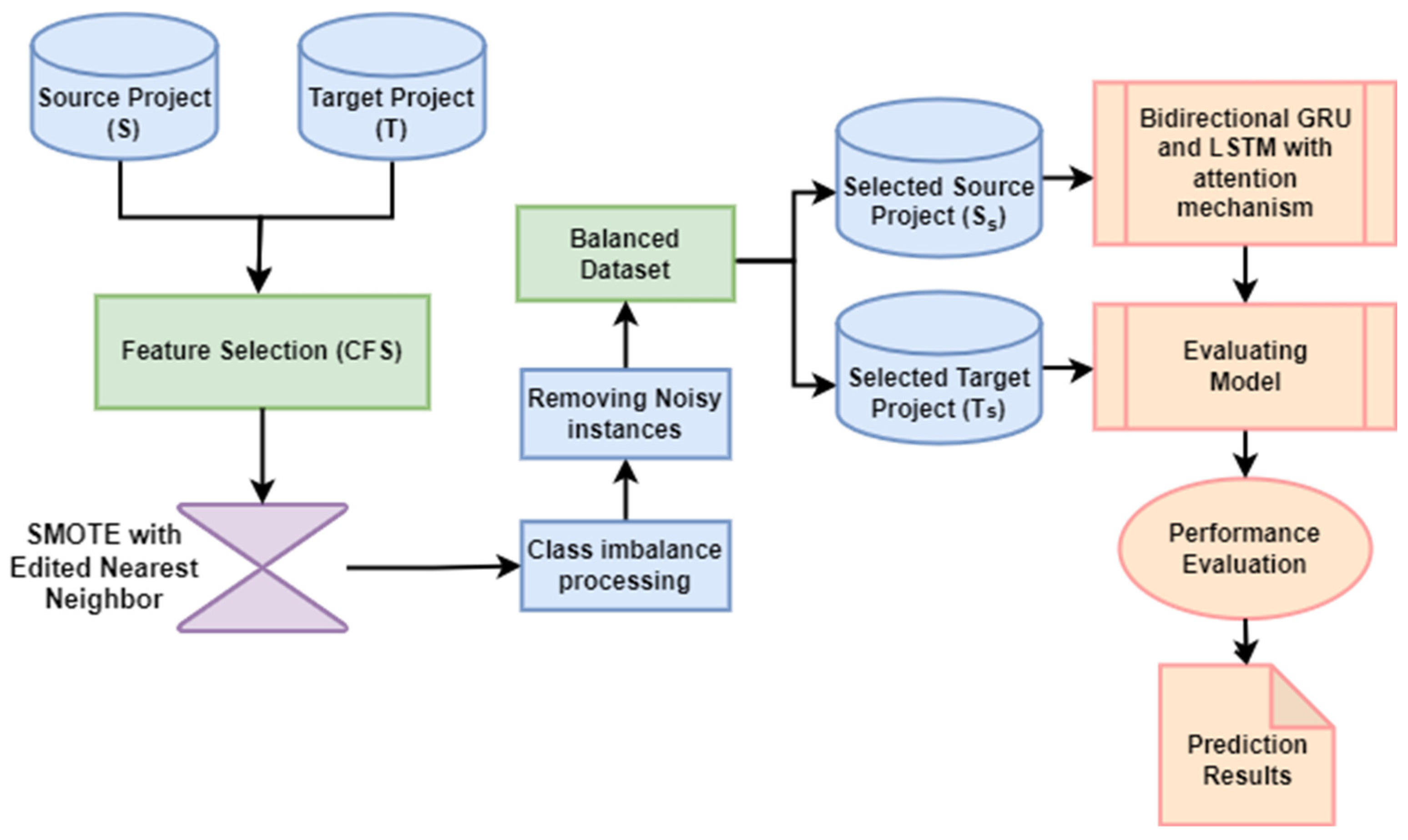
We illustrate our proposed approach for CPDP employing machine learning models (Bi-LSTM, Bi-GRU and Attention mechanism) combined with a feature selection method (CFS with best-first-search) and data sampling method (SMOTE-ENN) in this section. The datasets were obtained from the AEEEM and PROMISE as source (S) and target (T) projects. In order to select the features that are more relevant to the target class, feature selection is employed. Then a data balancing method is applied to balance the training dataset and remove noisy and irrelevant instances in source and target domains. Selected balanced source project (Ss) is then used to train the model. Finally, the trained model is utilized to predict the label of the selected balanced target project (Ts), and the result is then compared based on AUC and F1-measure performance metrics. Figure 1 demonstrates the full workflow of the proposed approach.

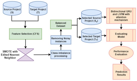
Figure 1. Overview of the proposed methodology for CPDP.

3.2. Proposed Features Selection Approach

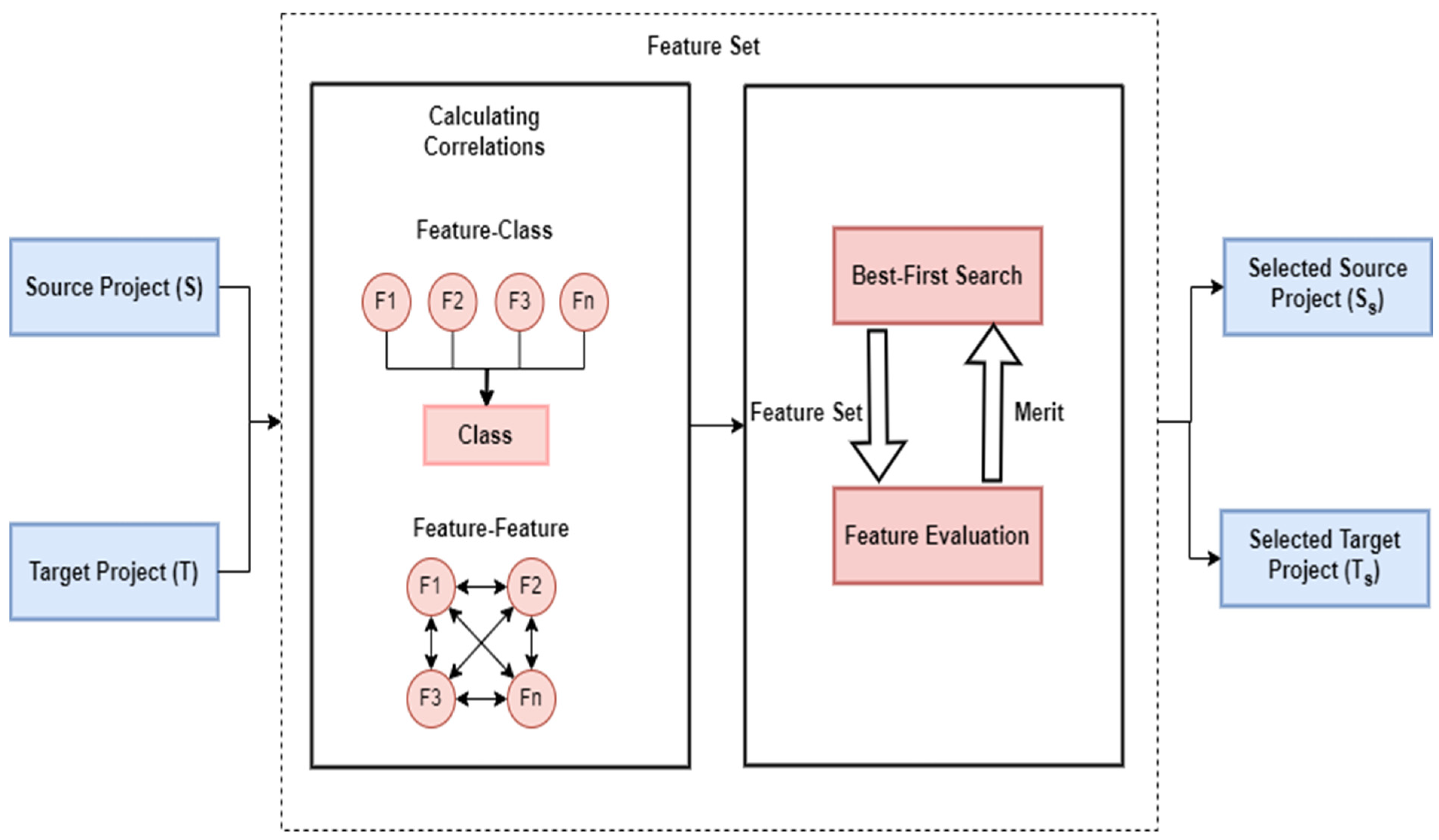
The prediction performance of CPDP models might be lowered by the presence of redundant or irrelevant features. By focusing on the most relevant features, the model may better capture the underlying patterns in the data and produce more accurate forecasts of defects in new projects [41]. We employ correlation-based feature selection (CFS) in the proposed framework, which chooses a subset of characteristics by taking into consideration each feature’s unique predictive capacity, as well as the degree of redundancy among them. The best-first search technique is employed to discover a feature subset in which these features have a strong correlation with regard to the target class labels, while having a low correlation within each other (Figure 2).

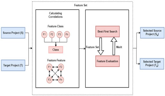
Figure 2. Workflow of CFS.

CFS begins by employing a correlation metric to determine the value of each individual feature $F$ and each feature set $f_1$, $f_2$, …, $f_n$, as illustrated in Algorithm 1. It initializes each feature as $f_i$ with the empty set $S$. Then, it selects the feature with the highest merits and adds it to the selected subset, while removing it from the remaining features. The process continues until the merit no longer changes considerably. Eventually, the algorithm returns the chosen subset S, which includes the most informative information for CPDP defect prediction.

Algorithm 1. Pseudocode of CFS

Input: - F, Feature set with n features, $=$ $f_1$, $f_2$, …, $f_n$ Output: - S, selected features Initialize an empty set S and sets $f_1$, $f_2$, …, $f_n$ with each feature $f_i$ Compute the merit of each feature $f_i$ in F. Compute the weight of each individual feature set ($f_1$, $f_2$, …, $f_n$) using a suitable metric (e.g., correlation). Select the feature with the highest weight from F, add it to S, and remove it from F Compute the weight of the current subset $S$ Select the new feature from $F$ with the highest merit, compute the merit of the updated subset, and compare it with the previous merit If the merit of the new subset is not better than the previous subset, Remove the selected feature from $S$ Else, Update $S$, remove the selected feature from $F$ Repeat steps 5–9 until the merit does not change significantly Return the selected features $S$

3.3. Proposed Imbalanced Learning Approach

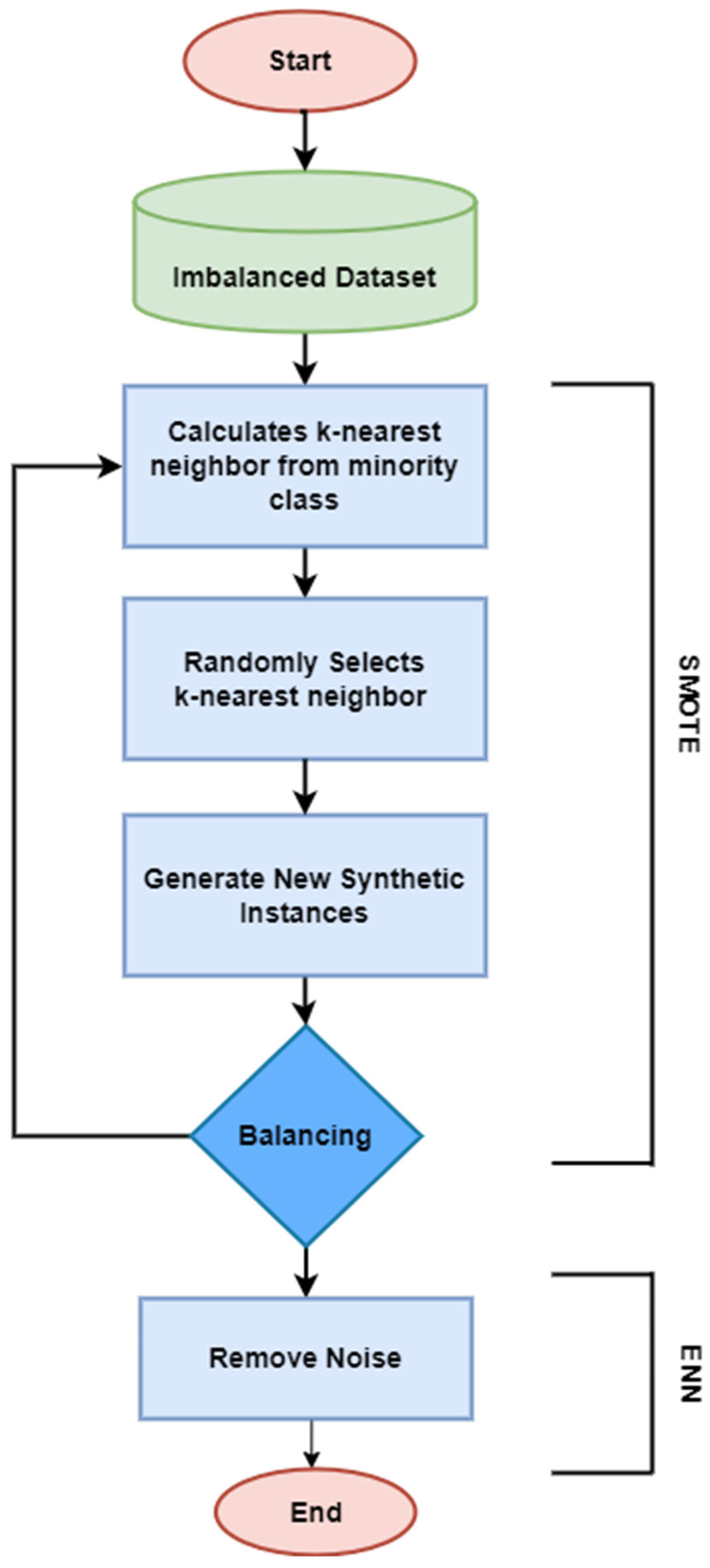
The term “class imbalance” refers to circumstances in which there are significantly fewer examples of one class than of others. Models trained on imbalanced datasets tend to exhibit a bias towards the majority class, leading to significant false negative rates, when real defects are neglected or misclassified as non-defective cases. Moreover, the addition of noisy and irrelevant occurrences among source and target projects also influences the prediction performance of CPDP models. A number of data balancing techniques have been developed to address the issue of imbalanced classes. Data sampling is the most widely used balancing approach. While undersampling approaches can lower the number of instances from the majority class [42], oversampling strategies can boost the representation of the minority class [43]. Our proposed approach uses the Synthetic Minority Oversampling Technique (SMOTE) [44] with Edited Nearest Neighbor (ENN) [45], which combines the ability of Edited Nearest Neighbor to clean data and the ability of SMOTE to generate synthetic data in order to produce a dataset that is more representative and balanced. As seen in Figure 3, the SMOTE-ENN approach consists of two basic steps: oversampling the minority class using SMOTE and cleaning the generated dataset using Edited Nearest Neighbor.

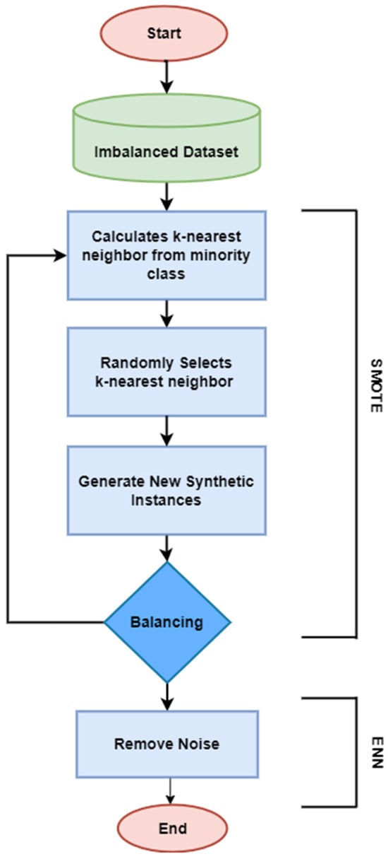
Figure 3. Flowchart of SMOTE-ENN.

The pseudocode of SMOTE-ENN is demonstrated in Algorithm 2. The SMOTE algorithm first separates minority $m\_i$ and majority $m\_a$ samples based on $y$ class labels and then determines the $k$ closest neighbors from the same class for each instance in the minority class $m\_i$. Then randomly choose one of the k nearest neighbors $\widehat{x}$ and compute the difference between the feature vectors of the instance and the selected neighbor $\left(\widehat{x}-x_i\right)$. Multiply this difference by a random value $\delta$ between 0 and 1 and add it to the feature vector of the instance $x_i$. This builds a synthetic instance $x_{new}$. After oversampling the minority class $m\_i$, the final dataset may still contain noisy and irrelevant instances. This is when the Edited Nearest Neighbor (ENN) algorithm comes into play. The ENN algorithm finds three nearest neighbors for each instance $x_j$ and removes instances $x_j$ that are misclassified by their nearest neighbors, hence improving the quality of the dataset.

Algorithm 2. Pseudocode of SMOTE Edited Nearest Neighbor (SMOTE-ENN)

Input: - X: Feature (samples(n) X features[n]) for both majority and minority classes - Y: Target variable (samples(n)) indicating class labels Output: - X_resampled: Resampled feature matrix after applying SMOTE-ENN - Y_resampled: Resampled target variable after applying SMOTE-ENN Separate minority and majority class as $m\_i$ and $m\_a$ Identify $m\_i$ and $m\_a$ samples based on class labels in $y$ For each $m\_i$ sample $x_i$, calculate, k-nearest neighbors. Select one of the random nearest neighbors $\widehat{x}$ Generate a new synthetic sample $x_{new}=x_i+\delta \left(\widehat{x}-x_i\right) where \delta ϵ\left[1\right]$ Repeat the above steps until the desired balance ratio is achieved For each instance $x_j$ in the augmented dataset: Find the three nearest neighbors of $x_j$ If $x_j$ is misclassified by its three nearest neighbors, delete $x_j$ Return Resampled Dataset

3.4. Model Building

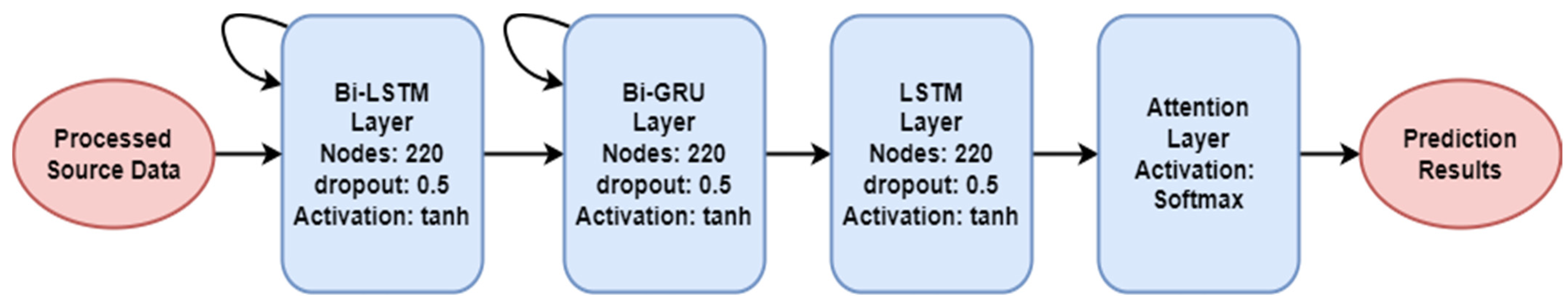
Our learning model architecture comprises four layers, starting with the Bi-LSTM layer which consists of 220 nodes. The second and third layers are Bi-GRU and LSTM, having 220 nodes each. For acquiring important features, we used the attention layer. All dense layers utilize the tanh as their activation function. The activation function applied in the last layer is softmax. The term “dropout” describes the possibility that any given node will be eliminated or dropped out, as seen in Figure 4. Algorithm 3 illustrates our model’s detail processing. In the proposed approach, for each source dataset $S\left[n\right]$, the CFS algorithm:

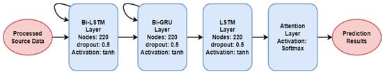
Figure 4. Architecture of the proposed model.

(1)

Calculates the merit of each feature and selects the top features based on the highest merit.

(2)

Selects the top k features based on the highest merit and creates the $S\_selected$ dataset.

The top k features are selected based on the highest merit values, and the $S\_selected$ dataset is created by combining the selected features from all source datasets. The merit of a feature f in a dataset $S$ can be calculated using the following Equation (1):

$$merit(f,S)=Metric(f,S),$$

(1)

where $Metric(f,S)$ is a feature selection correlation metric.

The selected features from all source datasets are combined to create the $S\_selected$ dataset. Then the CFS algorithm selects the features from the target dataset $T$ that correspond to the features selected for the source dataset $S\left[n\right]$. The selected features from all target datasets are combined to create the $T\_selected$ dataset. The $T\_selected$ dataset is created as in Equation (2):

$$T\_selected=\{f | f \in T and f \in S\_selected\},$$

(2)

where $f$ is a feature that exists in both the target dataset $T$ and the $S\_selected$ dataset.

To address class imbalance issues and remove noisy and irrelevant instances in the source and target datasets, the SMOTE-ENN (Synthetic Minority Over-sampling Technique—Edited Nearest Neighbors) technique is applied. SMOTE-ENN works by:

(1)

Generating synthetic samples of the minority class using the k-nearest neighbors’ algorithm.

(2)

Removing any noisy or redundant samples from the resampled dataset using the Edited Nearest Neighbors (ENN) algorithm.

The resampled datasets are denoted as $S\_resampled$ and $T\_resampled$. Then split the resampled source and target datasets into training and testing sets. The split is carried out using an 80:20 ratio, where 80% of the data are used for training, and 20% is used for testing. The training and testing sets are denoted as:

$$S\_x,S\_y (\mathrm{Source} \mathrm{dataset})$$

$$T\_x,T\_y (\mathrm{Target} \mathrm{dataset})$$

The algorithm builds a Sequential Neural Network model with the following layers:

(1)

Bi-LSTM (Bidirectional Long Short-Term Memory) with 220 nodes

(2)

Bi-GRU (Bidirectional Gated Recurrent Unit) with 220 nodes

(3)

LSTM with 220 nodes

(4)

Attention Layer

The Bi-LSTM and Bi-GRU layers are combined to optimize LSTM to capture the sequential and contextual information in the data. The attention layer is added to allow the model to focus on the most relevant parts of the input data when making predictions. Then, it trains the model using the $T\_resampled$ dataset. The training process can be represented by the following Equation (3):

$$Model.fit(T\_resampled),$$

(3)

where model is the sequential neural network model built in the previous step, and $T\_resampled$ is the resampled target dataset. Then, it uses the trained model to predict the defects in the $T\_y$ (testing) dataset. The prediction can be represented by the following Equation (4):

$$Result=Model.predict(T\_y),$$

(4)

where $Result$ is the predicted defects for the $T\_y$ dataset. The algorithm returns the Result as the final output, which represents the predicted defects for the target dataset $T\_y$.

The Bi-directional Long Short-Term Memory (LSTM) and Gated Recurrent (GRU) Layer: The suggested model first leverages a bi-directional LSTM network to learn the contextual and semantic features. Due to its ability to ease the vanishing gradient problem and depict long-term dependency, this model has been selected [46]. Bi-LSTM is an expansion of LSTMm which comprises two LSTM layers, one processing the sequence in the forward direction and the other in the backward. The sequence is processed in reverse order by the backward LSTM layer, whereas the sequence is processed from start to finish by the forward LSTM layer. To create the final output, the hidden states from both layers are concatenated [47]. The bi-LSTM is defined by Equations (5)–(7), where $\overrightarrow{h_t}$ is the state of the forward LSTM, $\overrightarrow{h_t}$ is the state of the backward LSTM, and ⊕ signifies the operation of concatenating two vectors. To generate the final hidden state $h_t$= [$\overrightarrow{h_t}$,$\overleftarrow{h_t}$] at time step t, the forward layer’s $\overrightarrow{h_t}$ final output and the $\overleftarrow{h_t}$ backward layer’s reverse output are merged. The Bi-directional Gated Recurrent Unit (Bi-GRU) has the ability to learn knowledge from prior and subsequent data when dealing with the present data. Two unidirectional GRUs pointing in different directions are used to determine the state of the bi-GRU model. One GRU starts at the beginning of the data series and goes forward, and another GRU starts at the end and moves backward. This makes it possible for information from the past and the future to affect the states that are currently in effect now. The bi-GRU is defined by Equations (8)–(10), where $\overrightarrow{h_t}$ is the state of the forward GRU, $\overleftarrow{h_t}$ is the state of the backward GRU, and ⊕ signifies the operation of concatenating two vectors. The model is able to produce more precise predictions because of this bi-directional representation, which records contextual information from both the past and the future.

$$\overrightarrow{h_t}={LSTM}_{fwd}(x_{t, }\overrightarrow{h_{t-1}}),$$

(5)

$$\overleftarrow{h_t}={LSTM}_{bwd}(x_{t, }\overleftarrow{h_{t+1}}),$$

(6)

$$h_t=\overrightarrow{h_t}\oplus \overleftarrow{h_t} ,$$

(7)

$$\overrightarrow{h_t}={GRU}_{fwd}(x_{t, }\overrightarrow{h_{t-1}}),$$

(8)

$$\overleftarrow{h_t}={GRU}_{bwd}(x_{t, }\overleftarrow{h_{t+1}}),$$

(9)

$$h_t=\overrightarrow{h_t}\oplus \overleftarrow{h_t},$$

(10)

Attention Layer: We embed the attention layer solely in order to amplify the influence of features and focus more on key features, as shown in Equation (11). First, we input the values $u_{it}$ representing the hidden states to be scaled.

$$u_{it}=\tanh \left(W_n\ast h_{it}+b_n\right),$$

(11)

Then, to identify the important sequence’s properties, $u_n$ is employed. The normalized adaptive weights are then produced by the model using a softmax process by computing the dot product between $u_{it}$ and $u_n,$ as shown in Equation (12).

$${\alpha }_{it}=Softmax \frac{\mathrm{e}\mathrm{x}\mathrm{p}(u_{it}^T\ast u_n)}{{\sum }_{t=1}exp(u_{it}^T\ast u_n)},$$

(12)

Ultimately, the sequence vector is generated by the weighted summation of each node, as shown in Equation (13).

$$S_i=\sum _{t=1}{\alpha }_{it}\ast h_{it}$$

(13)

Algorithm 3. Proposed Approach.

Input: - Source Datasets: {$S_1$, $S_2$, …, $S_n$} -Target Dataset: T Output: - Predicted Defects for T 1: Feature Selection for each source dataset (n): Calculate the merit (S_selected) for each feature in S(n) Select the top features based on highest merit and create S_selected end for 2: Select Features for Target Dataset T_selected = Features selected from T using the features selected in step 1 3: Handle Class Imbalance (SMOTE-ENN) S_resampled = Apply SMOTE-ENN to S_selected to handle class imbalance T_resampled = Apply SMOTE-ENN to T_selected to handle class imbalance 4: Split the Target Dataset S_x, S_y = Split (S_resampled, Size = 0.2) T_x, T_y = Split (T_resampled, Size = 0.2) 5: Build a Classifier Model = Sequential Neural Network - Layer 1: Bi-LSTM with 220 nodes - Layer 2: Bi-GRU with 220 nodes - Layer 3: LSTM with 220 nodes - Layer 4: Attention Layer 6: Train the Classifier Model.fit (T_resampled) 7: Predict Defects for T_y Result = Model.predict (T_y) 8: Output Return Result as Predicted Defects for T_y End

4. Experimental Setups

We provide a detailed description of our experimental setup in this part, together with benchmark datasets, evaluation metrics, baseline methods and research questions.

4.1. Benchmark Datasets

The experiments were conducted on 10 open-source software projects from AEEEM (five JAVA open-source projects) and PROMISE (five projects randomly picked from PROMISE). The difficulty of the software development process and the complexity of the software code is considered when assembling and gathering the AEEEM database by Dambros [48]. The PROMISE dataset, which contains the most varied project features, was created by Jureczko and Madeyski [49]. Table 2 presents the detailed information of selected projects, including the projects names, numbers of instances and the percentage of defective modules.

Table 2. Description of the datasets that we have chosen.

Dataset	Project	Number of Instances	Defective Instances %
AEEEM	EQ	325	39.692
	JDT	997	20.662
	LC	399	16.040
	ML	1862	13.158
	PDE	1492	14.008
PROMISE	Ivy2.0	352	11.36
	Poi3.0	442	64.09
	Xerces1.4	508	76.81
	Synapse1.2	256	33.63
	Xalan2.6	875	53.13

4.2. Evaluation Metrics

We analyze our suggested model performance based on two evaluation metrics, F1-measure and AUC. The F1-measure is a typical evaluation metric used to evaluate the performance of a classification model. It is the precision and recall harmonic mean that balances the two metrics, as shown in Equation (14):

$$F1–Measure=\frac{2(Precision\times Recall)}{Precision+Recall}$$

(14)

Area Under the Receiver Operating Characteristic curve (AUC) is used to evaluate the degree of differentiation obtained by the model. Decision thresholds, like recall and precision, are insensitive to this. All potential classification thresholds are represented by a graphic that shows the true positive rate on the y-axis and the false positive rate on the x-axis, as shown in Equation (15). The higher the AUC, the better the prediction:

$$AUC=\frac{{\mathsf{\Sigma }}_{{ins}_i ϵ Positive Class}rank\left({ins}_i\right)-\frac{M\left(M+1\right)}{2}}{M.N}$$

(15)

where the numbers of positive and negative cases are represented by M and N, and the average positive samples rank is ${\mathsf{\Sigma }}_{{ins}_i ϵ Positive Class}rank\left({ins}_i\right)$.

4.3. Baseline Models

To test the efficacy of our SCAG-LSTM method, a comparative analysis is conducted that evaluates its prediction performance against a total of six state-of-the-art CPDP approaches, three for AEEEM and three for PROMISE datasets. These approaches are detailed succinctly in Table 3.

Table 3. Summary of the Baseline models for comparison.

Baseline Models	Reference No.	Advantages	Disadvantages
TPTL [31]	Liu et al., 2019	The two-phase transfer learning model improves prediction accuracy and efficiency by utilizing transfer learning.	Generalizability is limited because of the concentration on a particular collection of defect datasets.
ALTRA [41]	Yuan et al., 2020	ALTRA employs utilization of active learning to overcome the data distribution differences across source and target projects.	Limits the validation on different datasets by just conducting empirical research on the PROMISE dataset.
DAKTSVMO [27]	Jin et al., 2021	Its ability to align the data distribution across different software projects allows for domain adaptation in CPDP.	Lack of comparison with different domain adaption approaches.
MSCPDP [50]	Zhao et al., 2022	Ability to leverage information from multiple sources projects for enhanced prediction accuracy.	Did not entirely outperform more advanced single-source single-target approaches.
TFIA [24]	Xing et al., 2022	Feature-level filtering strategy to improve data distribution differences between projects.	Doesn’t investigate how changing certain parameters affects the performance of the model
GBCPDP [34]	Abdu et al., 2023	Uses graph features taken from CFG and DDG to build a predictive model using LSTM, offering a systematic framework.	Relying exclusively on CFG and DDG as graph features could fail to capture all necessary context-relevant data for defect prediction.

4.4. Research Questions

In this section, we will discuss the motivations, along with the research problems. This work aims to address the following research questions.

RQ1: Does balancing data and removing noisy instances from data improve the performance of our proposed model SCAG-LSTM?

This research question investigates the effectiveness of our data-balancing method to improve the performance of the proposed model in CPDP.

RQ2: Does the feature selection approach suggested in this paper have any impact on the performance of the model SCAG-LSTM?

This research question analyzes the usefulness of our feature selection approach to improve the performance of the proposed model in CPDP.

RQ3: How effective is our SCAG-LSTM model? How much improvement can SCAG-LSTM achieve over the related models?

This research question seeks to determine how well the proposed method performs in CPDP in comparison to existing state-of-the-art approaches.

The motivation for the above mentioned research questions is driven by the implementation of feature selection and data balancing approaches in CPDP studies. The most recent CPDP research [22,23,24] indicates that, in order to make a model that can accurately predict defects and prevent the model from being biased toward the majority class, it is crucial to apply data balancing methods to handle the imbalanced nature of the dataset and remove noisy and irrelevant instances. Rao et al. [42] integrated an undersampling method to balance the imbalanced datasets. Sun et al. [51] explored undersampling techniques and proved that undersampling easily handles the imbalanced nature of the data. Moreover, feature selection methods reduce data distribution differences in order to increase the efficiency and efficacy of defect prediction models [52]. Lei et al. [53] introduced a cross project defect prediction technique based on feature selection and distance weight instance transfer. They showed the efficiency of feature selection on the suggested method. Zhao et al. [50] suggested a multi-source-based cross project defect prediction technique MSCPDP, which can handle the problem of data distribution differences between source and target domains.

5. Experimental Results

In this section, we present the experimental results and provide the answers to the research questions from Section 4.4.

5.1. Research Question—RQ1

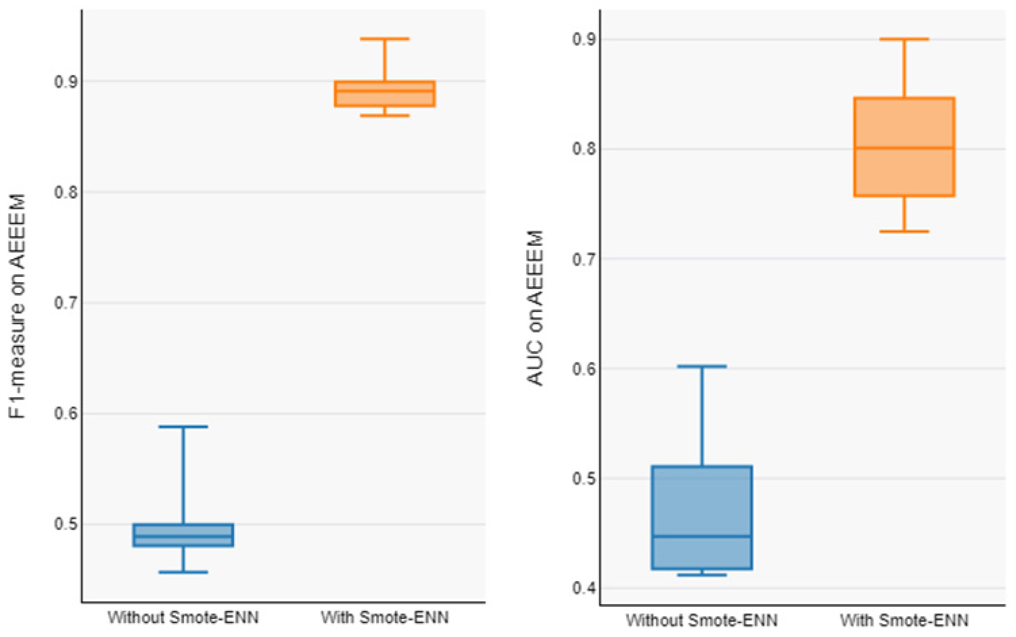
In order to address RQ1, Table 4 reports the proposed model’s performance on the AEEEM dataset with and without data balancing, and Table 5 reports the prediction model’s performance on the PROMISE dataset. Our model averages for the unbalanced datasets (F1-measure and AUC) are 0.503 and 0.466 for AEEEM and 0.380 and 0.510 for PROMISE. The average value of our proposed model on the balanced datasets (F1-measure and AUC) are 0.891 and 0.801 for AEEEM and 0.643 and 0.680 for PROMISE. From Table 3 and Table 4, it can be observed that the overall performance of the prediction model trained from the data processed by data balancing is significantly improved, with an average F1-measure improvement of about 77.34% and AUC improvement of about 71.98% on AEEEM and F1-measure improvement of about 69.21% and AUC improvement of about 33.33% on PROMISE, as compared to without data balancing. The Box plots of performance measures for the AEEEM datasets are shown in Figure 5 and Figure 6, displaying the performance measures for the PROMISE datasets with and without data balancing (F1-measure and AUC). Compared to the data without data balancing, we can observe that the prediction models trained using the data processed by data balancing have larger numerical intervals in the overall distribution. As a result, we can conclude that the data balancing strategy put forth in this study works well in enhancing the CPDP model’s performance across all datasets.

Table 4. F1-measure and AUC of proposed model with and without data balancing method on AEEEM.

Source	Target	F1-Measure		AUC
		Without SMOTE-ENN	With SMOTE-ENN	Without SMOTE-ENN	With SMOTE-ENN
EQ	JDT	0.580	0.900	0.447	0.875
EQ	LC	0.588	0.917	0.416	0.750
EQ	ML	0.563	0.895	0.413	0.731
EQ	PDE	0.457	0.879	0.412	0.771
JDT	EQ	0.578	0.892	0.602	0.900
JDT	LC	0.494	0.879	0.510	0.810
JDT	ML	0.489	0.887	0.427	0.762
JDT	PDE	0.483	0.875	0.420	0.761
LC	EQ	0.488	0.878	0.510	0.846
LC	JDT	0.491	0.923	0.515	0.848
LC	ML	0.481	0.869	0.422	0.738
LC	PDE	0.478	0.871	0.429	0.760
ML	EQ	0.480	0.893	0.513	0.848
ML	JDT	0.466	0.899	0.509	0.823
ML	LC	0.499	0.938	0.507	0.835
ML	PDE	0.487	0.873	0.418	0.750
PDE	EQ	0.489	0.908	0.514	0.883
PDE	JDT	0.497	0.891	0.412	0.791
PDE	LC	0.480	0.884	0.519	0.820
PDE	ML	0.495	0.877	0.415	0.725
Average		0.503	0.891	0.466	0.801

Table 5. F1-measure and AUC of proposed model with and without data balancing method on PROMISE.

Source	Target	F1-Measure		AUC
		Without SMOTE-ENN	With SMOTE-ENN	Without SMOTE-ENN	With SMOTE-ENN
synapse_1.2	poi-2.5	0.390	0.651	0.502	0.674
synapse_1.2	xerces-1.2	0.378	0.602	0.519	0.712
camel-1.4	ant-1.6	0.381	0.656	0.514	0.669
camel-1.4	jedit_4.1	0.378	0.636	0.480	0.612
xerces-1.3	poi-2.5	0.332	0.595	0.499	0.633
xerces-1.3	synapse_1.1	0.328	0.588	0.501	0.602
xerces-1.2	xalan-2.5	0.330	0.571	0.513	0.722
lucene_2.2	xalan-2.5	0.393	0.612	0.520	0.733
synapse_1.1	poi-3.0	0.387	0.602	0.497	0.630
ant-1.6	poi-3.0	0.319	0.520	0.460	0.619
camel-1.4	ant-1.6	0.430	0.782	0.537	0.713
lucene_2.2	ant-1.6	0.417	0.772	0.522	0.729
log4j-1.1	ant-1.6	0.415	0.745	0.528	0.733
log4j-1.1	lucene_2.0	0.402	0.733	0.527	0.757
lucene_2.0	log4j-1.1	0.449	0.742	0.560	0.719
lucene_2.0	xalan-2.5	0.342	0.546	0.501	0.669
jedit_4.1	camel-1.4	0.401	0.678	0.498	0.644
jedit_4.1	xalan-2.4	0.376	0.552	0.517	0.680
Average		0.380	0.643	0.510	0.680

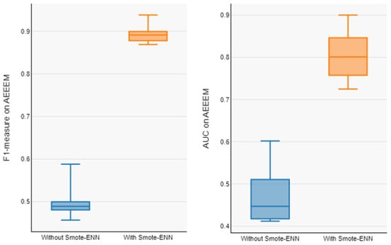
Figure 5. Boxplot of F1-measure and AUC of model with and without Smote-Enn on AEEEM.

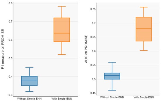
Figure 6. Boxplot of F1-measure and AUC of model with and without Smote-Enn on PROMISE.

5.2. Research Question—RQ2

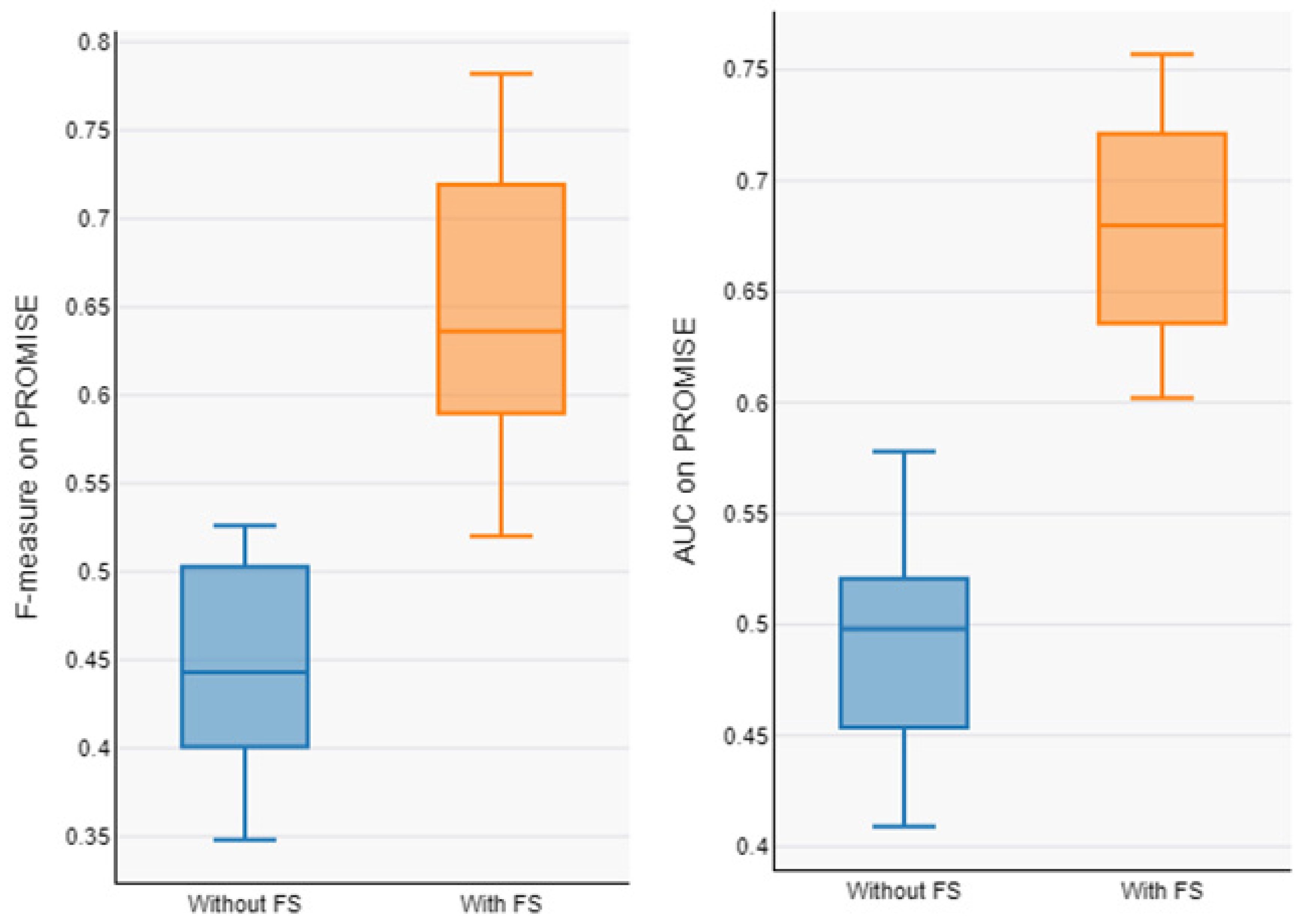
In order to address RQ2, Table 6 and Table 7 present the prediction model’s performance on the AEEEM and PROMISE dataset with and without feature selection. The average value of our model on the datasets without feature selection (F1-measure and AUC) are 0.678 and 0.637 on AEEEM and 0.443 and 0.496 on PROMISE. The average value of our model on the feature selected datasets (F1-measure and AUC) are 0.891 and 0.801 on AEEEM and 0.643 and 0.680 on PROMISE. From Table 5 and Table 6, it can be observed that the overall performance of the prediction model trained from the data processed by the feature selection is significantly improved, with an average F1-measure improvement of about 31.41% and AUC improvement of about 25.74% on AEEEM, and an F1-measure improvement of about 31.39% and AUC improvement of about 28.88% on PROMISE, as compared to without feature selection. The Box plots of performance measures for the AEEEM datasets are shown in Figure 7 and the Box plots of performance measures for the PROMISE datasets are shown in Figure 8, with and without feature selection (F1-measure and AUC). We observe that our proposed model shows good results on the feature-selected datasets, indicating that the proposed model performs well and that the feature selection method plays a significant role in enhancing prediction performance.

Table 6. F1-measure and AUC of proposed model with and without FS method on AEEEM.

Source	Target	F1-Measure		AUC
		Without FS	With FS	Without FS	With FS
EQ	JDT	0.737	0.900	0.681	0.875
EQ	LC	0.742	0.917	0.590	0.750
EQ	ML	0.677	0.895	0.589	0.731
EQ	PDE	0.659	0.879	0.610	0.771
JDT	EQ	0.668	0.892	0.719	0.900
JDT	LC	0.652	0.879	0.670	0.810
JDT	ML	0.661	0.887	0.680	0.762
JDT	PDE	0.649	0.875	0.586	0.761
LC	EQ	0.650	0.878	0.570	0.846
LC	JDT	0.760	0.923	0.674	0.848
LC	ML	0.643	0.869	0.571	0.738
LC	PDE	0.651	0.871	0.592	0.760
ML	EQ	0.665	0.893	0.688	0.848
ML	JDT	0.669	0.899	0.660	0.823
ML	LC	0.772	0.938	0.688	0.835
ML	PDE	0.644	0.873	0.580	0.750
PDE	EQ	0.733	0.908	0.699	0.883
PDE	JDT	0.665	0.891	0.629	0.791
PDE	LC	0.654	0.884	0.681	0.820
PDE	ML	0.628	0.877	0.588	0.725
Average		0.678	0.891	0.637	0.801

Table 7. F1-measure and AUC of proposed model with and without FS on PROMISE.

Source	Target	F1-Measure		AUC
		Without FS	With FS	Without FS	With FS
synapse_1.2	poi-2.5	0.422	0.651	0.450	0.674
synapse_1.2	xerces-1.2	0.409	0.602	0.508	0.712
camel-1.4	ant-1.6	0.419	0.656	0.498	0.669
camel-1.4	jedit_4.1	0.410	0.636	0.512	0.612
xerces-1.3	poi-2.5	0.390	0.595	0.445	0.633
xerces-1.3	synapse_1.1	0.357	0.588	0.409	0.602
xerces-1.2	xalan-2.5	0.348	0.571	0.521	0.722
lucene_2.2	xalan-2.5	0.452	0.612	0.578	0.733
synapse_1.1	poi-3.0	0.502	0.602	0.436	0.630
ant-1.6	poi-3.0	0.480	0.520	0.456	0.619
camel-1.4	ant-1.6	0.520	0.782	0.533	0.713
lucene_2.2	ant-1.6	0.518	0.772	0.513	0.729
log4j-1.1	ant-1.6	0.526	0.745	0.520	0.733
log4j-1.1	lucene_2.0	0.503	0.733	0.547	0.757
lucene_2.0	log4j-1.1	0.519	0.742	0.578	0.719
lucene_2.0	xalan-2.5	0.398	0.546	0.490	0.669
jedit_4.1	camel-1.4	0.457	0.678	0.453	0.644
jedit_4.1	xalan-2.4	0.350	0.552	0.495	0.680
Average		0.443	0.643	0.496	0.680

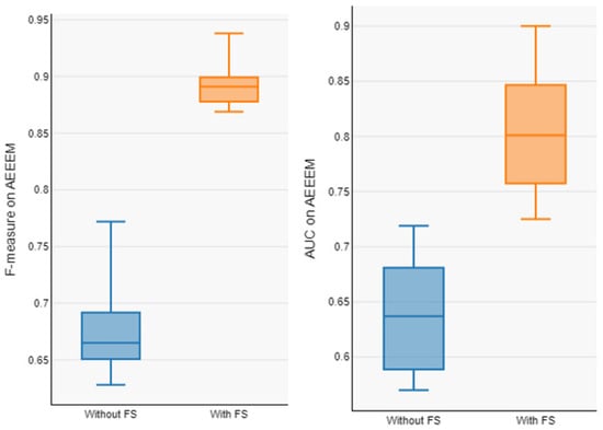
Figure 7. Boxplot of F1-measure and AUC of model with and without FS on AEEEM.

Figure 8. Boxplot of F1-measure and AUC of model with and without FS on PROMISE.

5.3. Research Question—RQ3

In order to address RQ3, we compared our model results with the results of baseline models based on two metrics: AUC and F1-measure. Table 8 and Table 9 compare the results of our model with the results of baseline models on AEEEM, and Table 10 and Table 11 compares the results of our model with the results of baseline models on PROMISE datasets. According to Table 7, Table 8, Table 9 and Table 10, our model outperforms the state-of-the art techniques and improves CPDP predictive performance. Figure 9 and Figure 10 display the Bar charts for prediction performance of the proposed model (SCAG-LSTM) and baseline models on the AEEEM and PROMISE datasets.

Table 8. F1-measure of the proposed approach and baseline methods on AEEEM.

Source	Target	ALTRA	MSCPDP	TFIA	Ours
EQ	JDT	0.448	0.411	0.873	0.900
EQ	LC	0.449	0.260	0.903	0.917
EQ	ML	0.304	0.244	0.875	0.895
EQ	PDE	0.415	0.260	0.864	0.879
JDT	EQ	0.526	0.266	0.862	0.892
JDT	LC	0.704	0.256	0.875	0.879
JDT	ML	0.725	0.259	0.883	0.887
JDT	PDE	0.713	0.283	0.866	0.875
LC	EQ	0.465	0.307	0.862	0.878
LC	JDT	0.868	0.486	0.911	0.923
LC	ML	0.862	0.298	0.855	0.869
LC	PDE	0.792	0.269	0.866	0.871
ML	EQ	0.710	0.162	0.886	0.893
ML	JDT	0.751	0.312	0.883	0.899
ML	LC	0.808	0.123	0.925	0.938
ML	PDE	0.806	0.227	0.865	0.873
PDE	EQ	0.644	0.233	0.897	0.908
PDE	JDT	0.800	0.391	0.881	0.891
PDE	LC	0.800	0.16	0.873	0.884
PDE	ML	0.800	0.219	0.853	0.877
Average		0.670	0.271	0.878	0.891

Table 9. AUC of the proposed approach and baseline methods on AEEEM.

Source	Target	ALTRA	MSCPDP	TFIA	Ours
EQ	JDT	0.266	0.628	0.735	0.875
EQ	LC	0.286	0.640	0.738	0.750
EQ	ML	0.253	0.557	0.702	0.731
EQ	PDE	0.203	0.557	0.740	0.771
JDT	EQ	0.388	0.575	0.719	0.900
JDT	LC	0.271	0.574	0.726	0.810
JDT	ML	0.605	0.574	0.707	0.762
JDT	PDE	0.668	0.583	0.721	0.761
LC	EQ	0.297	0.585	0.710	0.846
LC	JDT	0.441	0.667	0.768	0.848
LC	ML	0.341	0.590	0.732	0.738
LC	PDE	0.605	0.576	0.755	0.760
ML	EQ	0.579	0.528	0.755	0.848
ML	JDT	0.309	0.585	0.730	0.823
ML	LC	0.540	0.529	0.806	0.835
ML	PDE	0.287	0.558	0.724	0.750
PDE	EQ	0.373	0.551	0.785	0.883
PDE	JDT	0.388	0.620	0.754	0.791
PDE	LC	0.375	0.542	0.763	0.820
PDE	ML	0.491	0.558	0.718	0.725
Average		0.398	0.578	0.739	0.801

Table 10. F1-measure of the proposed approach and baseline methods on PROMISE.

Source	Target	TPTL	DA-KTSVMO	GB-CPDP	Ours
synapse_1.2	poi-2.5	0.462	0.533	0.631	0.651
synapse_1.2	xerces-1.2	0.433	0.542	0.466	0.602
camel-1.4	ant-1.6	0.575	0.463	0.416	0.656
camel-1.4	jedit_4.1	0.396	0.402	0.356	0.636
xerces-1.3	poi-2.5	0.349	0.537	0.544	0.595
xerces-1.3	synapse_1.1	0.536	0.329	0.469	0.588
xerces-1.2	xalan-2.5	0.447	0.462	0.383	0.571
lucene_2.2	xalan-2.5	0.506	0.438	0.502	0.612
synapse_1.1	poi-3.0	0.342	0.566	0.537	0.602
ant-1.6	poi-3.0	0.353	0.315	0.384	0.520
camel-1.4	ant-1.6	0.556	0.511	0.652	0.782
lucene_2.2	ant-1.6	0.377	0.539	0.669	0.772
log4j-1.1	ant-1.6	0.595	0.585	0.676	0.745
log4j-1.1	lucene_2.0	0.478	0.576	0.622	0.733
lucene_2.0	log4j-1.1	0.419	0.561	0.489	0.742
lucene_2.0	xalan-2.5	0.510	0.510	0.514	0.546
jedit_4.1	camel-1.4	0.447	0.502	0.501	0.678
jedit_4.1	xalan-2.4	0.332	0.386	0.443	0.552
Average		0.451	0.487	0.514	0.643

Table 11. AUC of the proposed approach and baseline methods on PROMISE.

Source	Target	TPTL	DA-KTSVMO	GB-CPDP	Ours
synapse_1.2	poi-2.5	0.485	0.498	0.593	0.674
synapse_1.2	xerces-1.2	0.485	0.563	0.681	0.712
camel-1.4	ant-1.6	0.541	0.655	0.532	0.669
camel-1.4	jedit_4.1	0.329	0.441	0.466	0.612
xerces-1.3	poi-2.5	0.588	0.477	0.568	0.633
xerces-1.3	synapse_1.1	0.488	0.468	0.502	0.602
xerces-1.2	xalan-2.5	0.471	0.437	0.696	0.722
lucene_2.2	xalan-2.5	0.621	0.702	0.568	0.733
synapse_1.1	poi-3.0	0.493	0.510	0.571	0.630
ant-1.6	poi-3.0	0.518	0.383	0.572	0.619
camel-1.4	ant-1.6	0.603	0.642	0.661	0.713
lucene_2.2	ant-1.6	0.411	0.570	0.658	0.729
log4j-1.1	ant-1.6	0.631	0.509	0.682	0.733
log4j-1.1	lucene_2.0	0.529	0.621	0.613	0.757
lucene_2.0	log4j-1.1	0.546	0.571	0.647	0.719
lucene_2.0	xalan-2.5	0.632	0.604	0.594	0.669
jedit_4.1	camel-1.4	0.267	0.355	0.556	0.644
jedit_4.1	xalan-2.4	0.425	0.563	0.669	0.680
Average		0.504	0.532	0.602	0.680

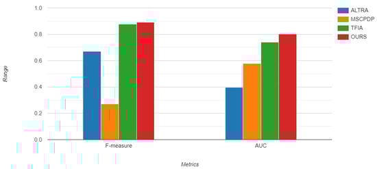
Figure 9. Bar chart of prediction performance of proposed model and comparing models on AEEEM.

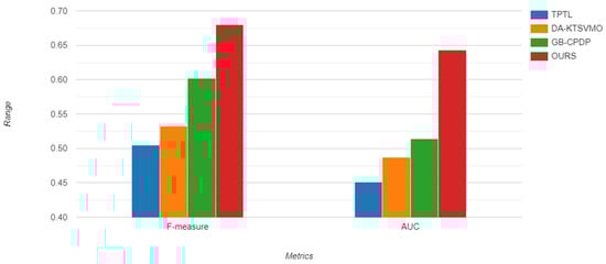
Figure 10. Bar chart of prediction performance of proposed model and comparative models on PROMISE.

6. Threats to Validity

6.1. Internal Validity

The degree of trust by which the causal relationship under investigation in a study is independent of other factors, or is unaffected by other variables, is known as internal validity. As a result, the accuracy of our testing setup is crucial to maintaining internal validity. TensorFlow serves as the backend for Keras, which we employ in this study to construct the SCAG-LSTM model. Since these technologies and tools have been used extensively in relevant research, they can be trusted. We additionally do white-box testing on the source code to ensure that it is error-free. Another important danger to internal validity comes from the datasets. The reference datasets are unbalanced and exhibit a deficiency in the true distribution of the fraction of classes that are defective and those that are not. In order to increase the data’s realism regarding the defect’s actual existence in the software system, we alter the original datasets to mitigate this threat. Data sampling strategies are used to modify the dataset’s distribution. However, we accept that many statistical tests can be performed to verify the statistical significance of our conclusions. Therefore, we propose to undertake more statistical testing in our future work.

6.2. External Validity

The term “external validity” describes a scientific research study’s ability to be transferred to other investigations. The primary risk to the external validity of this study is from our attempt to identify and collect diverse datasets from different AEEEM and PROMISE projects. For our evaluation datasets, we chose five open-source Java programs from the PROMISE and five open-source applications from the AEEEM dataset. We will be able to confirm the correctness of our strategy with additional experiments on different datasets. Furthermore, we cannot claim that our findings are broadly applicable. To ensure that the results of this study can be applied to a larger population, future replication is required.

6.3. Construct Validity

Construct validity pertains to the design of the study and its ability to accurately represent the true objective of the investigation. We have used a methodically related work evaluation technique to combat these hazards to our study design. We double-checked and made multiple adjustments to the research questions to make sure the topic was pertinent to the study’s objective. The metrics taken into consideration can also endanger our research. We use static code metrics exclusively for fault prediction. As a result, we are unable to say if our findings apply to additional parameters. Nevertheless, much earlier research also commonly used static code metrics. Further research on performance measures is planned. The creation of ML models is another danger. We looked at a number of factors that might have affected the study, such as feature selection, data pre-processing, data balancing techniques, how to train the models, and which features to evaluate. However, the methods used here are accurate enough to guarantee the validity of the study.

6.4. Conclusion Validity

The degree to which the research conclusion is derived in a reasonable manner is referred to as conclusion validity. We conducted numerous experiments on sufficient projects in this study to reduce the risk to the validity of the conclusions. As a result, the outcomes derived from the collected experimental data should be statistically reliable.

7. Conclusions and Future Work

Defect prediction and quality assurance are critical in today’s quickly changing software development environment to guarantee the stability and dependability of software projects. Predicting errors across many software projects with accuracy and efficiency is a major challenge in this industry. In order to improve the predictive performance of the cross-project defect prediction (CPDP) model, we combined a variety of data preprocessing, feature selection, data sampling, and modeling approaches in our study to propose a comprehensive approach to addressing the difficulties associated with CPDP. To improve the existing state-of-the-art approaches to predicting software defects, we proposed a novel domain adaptive approach, which first integrates CFS-BFS and SMOTE-ENN to overcome the domain adaptive problems related to data distribution differences and imbalance class, enhancing the model’s performance and making it more robust and capable of handling real-world software defect prediction scenarios. Furthermore, it optimizes LSTM with Bi-GRU and Attention Mechanism to capture complex patterns and dependencies in the data, while the attention layer provided insights into which features and instances are most influential in making predictions. We conducted a number of tests on 10 publicly available apache_lucene, equinox, eclipse_jdt_core, eclipse_pde_ui, and mylyn (AEEEM) and predictor models in software engineering (PROMISE) datasets in order to assess the efficacy of the suggested models, i.e., the baseline models, active learning-based method (ALTRA), multi-source-based cross-project defect prediction method (MSCPDP), two-phase feature importance amplification method (TFIA), domain adaptive kernel twin support vector machines method (DA-KTSVMO), two-phase transfer learning method (TPTL), and generative adversarial long-short term memory neural networks method (GB-CPDP) and the outcomes were contrasted. According to our findings, the suggested model outperforms the baseline models by 33.03%, 29.15% and 1.48% in terms of F1-measure and by 16.32%, 34.41% and 3.59% in terms of Area Under the Curve (AUC) on the AEEEM dataset, while on the PROMISE dataset it enhances the baseline model F1-measure by 42.60%, 32.00% and 25.10% and AUC by 34.90%, 27.80% and 12.96% on the feature-selected and balanced datasets. Future studies and advancements have multiple directions to pursue. The suggested model can be strengthened and made more robust and generalizable by validating its performance on additional datasets. Secondly, since SCAG-LSTM is limited to one-to-one prediction, we could attempt research on the many-to-one scenarios in the future.

References

- Khan, M.A.; Elmitwally, N.S.; Abbas, S.; Aftab, S.; Ahmad, M.; Fayaz, M.; Khan, F. Software defect prediction using artificial neural networks: A systematic literature review. Sci. Program. 2022, 2022, 2117339. [Google Scholar] [CrossRef]
- Alenezi, M. Internal quality evolution of open-source software systems. Appl. Sci. 2021, 11, 5690. [Google Scholar] [CrossRef]
- Aljumah, S.; Berriche, L. Bi-LSTM-based neural source code summarization. Appl. Sci. 2022, 12, 12587. [Google Scholar] [CrossRef]
- Alqmase, M.; Alshayeb, M.; Ghouti, L. Quality assessment framework to rank software projects. Autom. Softw. Eng. 2022, 29, 41. [Google Scholar] [CrossRef]
- Akimova, E.N.; Bersenev, A.Y.; Deikov, A.A.; Kobylkin, K.S.; Konygin, A.V.; Mezentsev, I.P.; Misilov, V.E. A survey on software defect prediction using deep learning. Mathematics 2021, 9, 1180. [Google Scholar] [CrossRef]
- Thota, M.K.; Shajin, F.H.; Rajesh, P. Survey on software defect prediction techniques. Int. J. Appl. Sci. Eng. 2020, 17, 331–344. [Google Scholar]
- Matloob, F.; Ghazal, T.M.; Taleb, N.; Aftab, S.; Ahmad, M.; Khan, M.A.; Abbas, S.; Soomro, T.R. Software defect prediction using ensemble learning: A systematic literature review. IEEE Access 2021, 9, 98754–98771. [Google Scholar] [CrossRef]
- Gong, L.N.; Jiang, S.J.; Jiang, L. Research progress of software defect prediction. J. Softw. 2019, 30, 3090–3114. [Google Scholar]
- Pal, S.; Sillitti, A. A classification of software defect prediction models. In Proceedings of the 2021 International Conference Nonlinearity, Information and Robotics (NIR), Innopolis, Russia, 26–29 August 2021; pp. 1–6. [Google Scholar]
- Pan, C.; Lu, M.; Xu, B.; Gao, H. An improved CNN model for within-project software defect prediction. Appl. Sci. 2019, 9, 2138. [Google Scholar] [CrossRef]
- Bhat, N.A.; Farooq, S.U. An empirical evaluation of defect prediction approaches in within-project and cross-project context. Softw. Qual. J. 2023, 31, 917–946. [Google Scholar] [CrossRef]
- Malhotra, R.; Khan, A.A.; Khera, A. Simplify Your Neural Networks: An Empirical Study on Cross-Project Defect Prediction. In Proceedings of the Computer Networks and Inventive Communication Technologies: Fourth ICCNCT 2021, Coimbatore, India, 1–2 April 2022; pp. 85–98. [Google Scholar]
- Vescan, A.; Găceanu, R. Cross-Project Defect Prediction using Supervised and Unsupervised Learning: A Replication Study. In Proceedings of the 2023 27th International Conference on System Theory, Control and Computing (ICSTCC), Timisoara, Romania, 11–13 October 2023; pp. 440–447. [Google Scholar]
- Sasankar, P.; Sakarkar, G. Cross-Project Defect Prediction: Leveraging Knowledge Transfer for Improved Software Quality Assurance. In Proceedings of the International Conference on Electrical and Electronics Engineering, Barcelona, Spain, 19–21 August 2023; pp. 291–303. [Google Scholar]
- Jing, X.-Y.; Chen, H.; Xu, B. Cross-Project Defect Prediction. In Intelligent Software Defect Prediction; Springer: Berlin/Heidelberg, Germany, 2024; pp. 35–63. [Google Scholar]
- Bala, Y.Z.; Samat, P.A.; Sharif, K.Y.; Manshor, N. Cross-project software defect prediction through multiple learning. Bull. Electr. Eng. Inform. 2024, 13, 2027–2035. [Google Scholar] [CrossRef]
- Tao, H.; Fu, L.; Cao, Q.; Niu, X.; Chen, H.; Shang, S.; Xian, Y. Cross-Project Defect Prediction Using Transfer Learning with Long Short-Term Memory Networks. IET Softw. 2024, 2024, 5550801. [Google Scholar] [CrossRef]
- Fan, X.; Zhang, S.; Wu, K.; Zheng, W.; Ge, Y. Cross-Project Software Defect Prediction Based on SMOTE and Deep Canonical Correlation Analysis. Comput. Mater. Contin. 2024, 78, 1687–1711. [Google Scholar] [CrossRef]
- Saeed, M.S.; Saleem, M. Cross Project Software Defect Prediction Using Machine Learning: A Review. Int. J. Comput. Innov. Sci. 2023, 2, 35–52. [Google Scholar]
- Malhotra, R.; Meena, S. Empirical validation of feature selection techniques for cross-project defect prediction. Int. J. Syst. Assur. Eng. Manag. 2023, 1–13. [Google Scholar] [CrossRef]
- Xing, Y.; Qian, X.; Guan, Y.; Yang, B.; Zhang, Y. Cross-project defect prediction based on G-LSTM model. Pattern Recognit. Lett. 2022, 160, 50–57. [Google Scholar] [CrossRef]
- Pandey, S.K.; Tripathi, A.K. Class imbalance issue in software defect prediction models by various machine learning techniques: An empirical study. In Proceedings of the 2021 8th International Conference on Smart Computing and Communications (ICSCC), Kochi, India, 1–3 July 2021. [Google Scholar]
- Goel, L.; Sharma, M.; Khatri, S.K.; Damodaran, D. Cross-project defect prediction using data sampling for class imbalance learning: An empirical study. Int. J. Parallel Emergent Distrib. Syst. 2021, 36, 130–143. [Google Scholar] [CrossRef]
- Xing, Y.; Lin, W.; Lin, X.; Yang, B.; Tan, Z. Cross-project defect prediction based on two-phase feature importance amplification. Comput. Intell. Neurosci. 2022, 2022, 2320447. [Google Scholar] [CrossRef] [PubMed]
- Goel, L.; Nandal, N.; Gupta, S. An optimized approach for class imbalance problem in heterogeneous cross project defect prediction. F1000Research 2022, 11, 1060. [Google Scholar] [CrossRef]
- Nevendra, M.; Singh, P. Cross-Project Defect Prediction with Metrics Selection and Balancing Approach. Appl. Comput. Syst. 2022, 27, 137–148. [Google Scholar] [CrossRef]
- Jin, C. Cross-project software defect prediction based on domain adaptation learning and optimization. Expert Syst. Appl. 2021, 171, 114637. [Google Scholar] [CrossRef]
- Sun, Z.; Li, J.; Sun, H.; He, L. CFPS: Collaborative filtering based source projects selection for cross-project defect prediction. Appl. Soft Comput. 2021, 99, 106940. [Google Scholar] [CrossRef]
- Saeed, M.S. Role of Feature Selection in Cross Project Software Defect Prediction—A Review. Int. J. Comput. Inf. Manuf. (IJCIM) 2023, 3, 37–56. [Google Scholar]
- Khatri, Y.; Singh, S.K. An effective feature selection based cross-project defect prediction model for software quality improvement. Int. J. Syst. Assur. Eng. Manag. 2023, 14 (Suppl. S1), 154–172. [Google Scholar] [CrossRef]
- Liu, C.; Yang, D.; Xia, X.; Yan, M.; Zhang, X. A two-phase transfer learning model for cross-project defect prediction. Inf. Softw. Technol. 2019, 107, 125–136. [Google Scholar] [CrossRef]
- Xu, Z.; Li, L.; Yan, M.; Liu, J.; Luo, X.; Grundy, J.; Zhang, Y.; Zhang, X. A comprehensive comparative study of clustering-based unsupervised defect prediction models. J. Syst. Softw. 2021, 172, 110862. [Google Scholar] [CrossRef]
- Ni, C.; Liu, W.-S.; Chen, X.; Gu, Q.; Chen, D.-X.; Huang, Q.-G. A cluster based feature selection method for cross-project software defect prediction. J. Comput. Sci. Technol. 2017, 32, 1090–1107. [Google Scholar] [CrossRef]
- Abdu, A.; Zhai, Z.; Abdo, H.A.; Algabri, R.; Lee, S. Graph-Based Feature Learning for Cross-Project Software Defect Prediction. Comput. Mater. Contin. 2023, 77, 161–180. [Google Scholar] [CrossRef]
- Goyal, S. Handling class-imbalance with KNN (neighbourhood) under-sampling for software defect prediction. Artif. Intell. Rev. 2022, 55, 2023–2064. [Google Scholar] [CrossRef]
- Kaur, H.; Pannu, H.S.; Malhi, A.K. A systematic review on imbalanced data challenges in machine learning: Applications and solutions. ACM Comput. Surv. (CSUR) 2019, 52, 1–36. [Google Scholar] [CrossRef]
- Bennin, K.E.; Keung, J.; Phannachitta, P.; Monden, A.; Mensah, S. Mahakil: Diversity based oversampling approach to alleviate the class imbalance issue in software defect prediction. IEEE Trans. Softw. Eng. 2017, 44, 534–550. [Google Scholar] [CrossRef]
- Vuttipittayamongkol, P.; Elyan, E. Neighbourhood-based undersampling approach for handling imbalanced and overlapped data. Inf. Sci. 2020, 509, 47–70. [Google Scholar] [CrossRef]
- Gong, L.; Jiang, S.; Jiang, L. An improved transfer adaptive boosting approach for mixed-project defect prediction. J. Softw. Evol. Process 2019, 31, e2172. [Google Scholar] [CrossRef]
- Kumar, A.; Kaur, A.; Singh, P.; Driss, M.; Boulila, W. Efficient Multiclass Classification Using Feature Selection in High-Dimensional Datasets. Electronics 2023, 12, 2290. [Google Scholar] [CrossRef]
- Yuan, Z.; Chen, X.; Cui, Z.; Mu, Y. ALTRA: Cross-project software defect prediction via active learning and tradaboost. IEEE Access 2020, 8, 30037–30049. [Google Scholar] [CrossRef]
- Rao, K.N.; Reddy, C.S. A novel under sampling strategy for efficient software defect analysis of skewed distributed data. Evol. Syst. 2020, 11, 119–131. [Google Scholar] [CrossRef]
- Fan, G.; Diao, X.; Yu, H.; Yang, K.; Chen, L. Software defect prediction via attention-based recurrent neural network. Sci. Program. 2019, 2019, 6230953. [Google Scholar] [CrossRef]
- Chawla, N.V.; Bowyer, K.W.; Hall, L.O.; Kegelmeyer, W.P. SMOTE: Synthetic minority over-sampling technique. J. Artif. Intell. Res. 2002, 16, 321–357. [Google Scholar] [CrossRef]
- Tomek, I. An Experiment with the Edited Nearest-Nieghbor Rule. IEEE Trans. Syst. Man Cybern 1976, 6, 448–452. [Google Scholar]
- Farid, A.B.; Fathy, E.M.; Eldin, A.S.; Abd-Elmegid, L.A. Software defect prediction using hybrid model (CBIL) of convolutional neural network (CNN) and bidirectional long short-term memory (Bi-LSTM). PeerJ Comput. Sci. 2021, 7, e739. [Google Scholar] [CrossRef]
- Uddin, M.N.; Li, B.; Ali, Z.; Kefalas, P.; Khan, I.; Zada, I. Software defect prediction employing BiLSTM and BERT-based semantic feature. Soft Comput. 2022, 26, 7877–7891. [Google Scholar] [CrossRef]
- D’Ambros, M.; Lanza, M.; Robbes, R. An extensive comparison of bug prediction approaches. In Proceedings of the 2010 7th IEEE Working Conference on Mining Software Repositories (MSR 2010), Cape Town, South Africa, 2–3 May 2010; pp. 31–41. [Google Scholar]
- Jureczko, M.; Madeyski, L. Towards identifying software project clusters with regard to defect prediction. In Proceedings of the 6th International Conference on Predictive Models in Software Engineering, Timișoara, Romania, 12–13 September 2010; pp. 1–10. [Google Scholar]
- Zhao, Y.; Zhu, Y.; Yu, Q.; Chen, X. Cross-project defect prediction considering multiple data distribution simultaneously. Symmetry 2022, 14, 401. [Google Scholar] [CrossRef]
- Sun, Z.; Zhang, J.; Sun, H.; Zhu, X. Collaborative filtering based recommendation of sampling methods for software defect prediction. Appl. Soft Comput. 2020, 90, 106163. [Google Scholar] [CrossRef]
- Palatse, V.G. Exploring principal component analysis in defect prediction: A survey. Perspect. Commun. Embed.-Syst. Signal-Process.-PiCES 2020, 4, 56–63. [Google Scholar]
- Lei, T.; Xue, J.; Wang, Y.; Niu, Z.; Shi, Z.; Zhang, Y. WCM-WTrA: A Cross-Project Defect Prediction Method Based on Feature Selection and Distance-Weight Transfer Learning. Chin. J. Electron. 2022, 31, 354–366. [Google Scholar] [CrossRef]
Disclaimer/Publisher’s Note: The statements, opinions and data contained in all publications are solely those of the individual author(s) and contributor(s) and not of MDPI and/or the editor(s). MDPI and/or the editor(s) disclaim responsibility for any injury to people or property resulting from any ideas, methods, instructions or products referred to in the content. |
© 2024 by the authors. Licensee MDPI, Basel, Switzerland. This article is an open access article distributed under the terms and conditions of the Creative Commons Attribution (CC BY) license (https://creativecommons.org/licenses/by/4.0/).