Abstract
Bayesian networks (BNs) are a foundational model in machine learning and causal inference. Their graphical structure can handle high-dimensional problems, divide them into a sparse collection of smaller ones, underlies Judea Pearl’s causality, and determines their explainability and interpretability. Despite their popularity, there are almost no resources in the literature on how to compute Shannon’s entropy and the Kullback–Leibler (KL) divergence for BNs under their most common distributional assumptions. In this paper, we provide computationally efficient algorithms for both by leveraging BNs’ graphical structure, and we illustrate them with a complete set of numerical examples. In the process, we show it is possible to reduce the computational complexity of KL from cubic to quadratic for Gaussian BNs.
1. Introduction
Bayesian networks [1] (BNs) have played a central role in machine learning research since the early days of the field as expert systems [2,3], graphical models [4,5], dynamic and latent variables models [6], and as the foundation of causal discovery [7] and causal inference [8]. They have also found applications as diverse as comorbidities in clinical psychology [9], the genetics of COVID-19 [10], the Sustainable Development Goals of the United Nations [11], railway disruptions [12] and industry 4.0 [13].
Machine learning, however, has evolved to include a variety of other models and reformulated them into a very general information-theoretic framework. The central quantities of this framework are Shannon’s entropy and the Kullback–Leibler divergence. Learning models from data relies crucially on the former to measure the amount of information captured by the model (or its complement, the amount of information lost in the residuals) and on the latter as the loss function we want to minimise. For instance, we can construct variational inference [14], the Expectation-Maximisation algorithm [15], Expectation Propagation [16] and various dimensionality reduction approaches such as t-SNE [17] and UMAP [18] using only these two quantities. We can also reformulate classical maximum-likelihood and Bayesian approaches to the same effect, from logistic regression to kernel methods to boosting [19,20].
Therefore, the lack of literature on how to compute the entropy of a BN and the Kullback–Leibler divergence between two BNs is surprising. While both are mentioned in Koller and Friedman [5] and discussed at a theoretical level in Moral et al. [21] for discrete BNs, no resources are available on any other type of BN. Furthermore, no numerical examples of how to compute them are available even for discrete BNs. We fill this gap in the literature by:
- Deriving efficient formulations of Shannon’s entropy and the Kullback–Leibler divergence for Gaussian BNs and conditional linear Gaussian BNs.
- Exploring the computational complexity of both for all common types of BNs.
- Providing step-by-step numeric examples for all computations and all common types of BNs.
Our aim is to make apparent how both quantities are computed in their closed-form exact expressions and what is the associated computational cost.
The common alternative is to estimate both Shannon’s entropy and the Kullback–Leibler divergence empirically using Monte Carlo sampling. Admittedly, this approach is simple to implement for all types of BNs. However, it has two crucial drawbacks:
- Using asymptotic estimates voids the theoretical properties of many machine learning algorithms: Expectation-Maximisation is not guaranteed to converge [5], for instance.
- The number of samples required to estimate the Kullback–Leibler divergence accurately on the tails of the global distribution of both BNs is also an issue [22], especially when we need to evaluate it repeatedly as part of some machine learning algorithm. The same is true, although to a lesser extent, for Shannon’s entropy as well. In general, the rate of convergence to the true posterior in Monte Carlo particle filters is proportional to the number of variables squared [23].
Therefore, efficiently computing the exact value of Shannon’s entropy and the Kullback–Leibler divergence is a valuable research endeavour with a practical impact on BN use in machine learning. To help its development, we implemented the methods proposed in the paper in our bnlearn R package [24].
The remainder of the paper is structured as follows. In Section 2, we provide the basic definitions, properties and notation of BNs. In Section 3, we revisit the most common distributional assumptions in the BN literature: discrete BNs (Section 3.1), Gaussian BNs (Section 3.2) and conditional linear Gaussian BNs (Section 3.3). We also briefly discuss exact and approximate inferences for these types of BNs in Section 3.4 to introduce some key concepts for later use. In Section 4, we discuss how we can compute Shannon’s entropy and the Kullback–Leibler divergence for each type of BN. We conclude the paper by summarising and discussing the relevance of these foundational results in Section 5. Appendix A summarises all the computational complexity results from earlier sections, and Appendix B contains additional examples we omitted from the main text for brevity.
2. Bayesian Networks
Bayesian networks (BNs) are a class of probabilistic graphical models defined over a set of random variables , each describing some quantity of interest, that are associated with the nodes of a directed acyclic graph (DAG) . Arcs in express direct dependence relationships between the variables in , with graphical separation in implying conditional independence in probability. As a result, induces the factorisation
in which the global distribution (of , with parameters ) decomposes into one local distribution for each (with parameters , ) conditional on its parents .
This factorisation is as effective at reducing the computational burden of working with BNs as the DAG underlying the BN is sparse, meaning that each node has a small number of parents (, usually with ). For instance, learning BNs from data is only feasible in practice if this holds. The task of learning a BN from a data set containing n observations comprises two steps:
If we assume that parameters in different local distributions are independent [25], we can perform parameter learning independently for each node. Each will have a low-dimensional parameter space , making parameter learning computationally efficient. On the other hand, structure learning is well known to be both NP-hard [26] and NP-complete [27], even under unrealistically favourable conditions such as the availability of an independence and inference oracle [28]. However, if is sparse, heuristic learning algorithms have been shown to run in quadratic time [29]. Exact learning algorithms, which have optimality guarantees that heuristic algorithms lack, retain their exponential complexity but become feasible for small problems because sparsity allows for tight bounds on goodness-of-fit scores and the efficient pruning of the space of the DAGs [30,31,32].
3. Common Distributional Assumptions for Bayesian Networks
While there are many possible choices for the distribution of in principle, the literature has focused on three cases.
3.1. Discrete BNs
Discrete BNs [25] assume that both and the are multinomial random variables (The literature sometimes denotes discrete BNs as “dBNs” or “DBNs”; we do not do that in this paper to avoid confusion with dynamic BNs, which are also commonly denoted as “dBNs”). Local distributions take the form
their parameters are the conditional probabilities of given each configuration of the values of its parents, usually represented as a conditional probability table (CPT) for each . The can be estimated from data via the sufficient statistic , the corresponding counts tallied from using maximum likelihood, Bayesian or shrinkage estimators as described in Koller and Friedman [5] and Hausser and Strimmer [33].
The global distribution takes the form of an N-dimensional probability table with one dimension for each variable. Assuming that each takes at most l values, the table will contain cells, where denotes the possible (configurations of the) values of its argument. As a result, it is impractical to use for medium and large BNs. Following standard practices from categorical data analysis [34], we can produce the CPT for each from the global distribution by marginalising (that is, summing over) all the variables other than and then normalising over each configuration of . Conversely, we can compose the global distribution from the local distributions of the by multiplying the appropriate set of conditional probabilities. The computational complexity of the composition is because applying (1) for each of the cells yields
which involves N multiplications. As for the decomposition, for each node, we:
- Sum over variables to produce the joint probability table for , which contains cells. The value of each cell is the sum of probabilities.
- Normalise the columns of the joint probability table for over each of the configurations of values of , which involves summing O(l) probabilities and dividing them by their total.
The resulting computational complexity is
for each node and for the whole BN.
Example 1
(Composing and decomposing a discrete BN). For reasons of space, this example is presented as Example A1 in Appendix B.
3.2. Gaussian BNs
Gaussian BNs [35] (GBNs) model with a multivariate normal random variable N(, and assume that the are univariate normals linked by linear dependencies,
which can be equivalently written as linear regression models of the form
The parameters in (3) and (4) are the regression coefficients associated with the parents , an intercept term and the variance . They are usually estimated by maximum likelihood, but Bayesian and regularised estimators are available as well [1].
The link between the parameterisation of the global distribution of a GBN and that of its local distributions is detailed in Pourahmadi [36]. We summarise it here for later use.
- Composing the global distribution. We can create an lower triangular matrix from the regression coefficients in the local distributions such that gives after rearranging rows and columns. In particular, we:
- Arrange the nodes of in the (partial) topological ordering induced by , denoted .
- The ith row of (denoted ], i = 1, …, N) is associated with X(i). We compute its elements from the parameters of X(i) | aswhere ] are the rows of that correspond to the parents of X(i). The rows of are filled following the topological ordering of the BN.
- Compute .
- Rearrange the rows and columns of to obtain .
Intuitively, we construct by propagating the node variances along the paths in while combining them with the regression coefficients, which are functions of the correlations between adjacent nodes. As a result, gives after rearranging the rows and columns to follow the original ordering of the nodes.The elements of the mean vector are similarly computed as iterating over the variables in topological order. - Decomposing the global distribution. Conversely, we can derive the matrix from by reordering its rows and columns to follow the topological ordering of the variables in and computing its Cholesky decomposition. Thencontains the regression coefficients in the elements corresponding to (Here is a diagonal matrix with the same diagonal elements as and is the identity matrix.) Finally, we compute the intercepts as by reversing the equations we used to construct above.
The computational complexity of composing the global distribution is bound by the matrix multiplication , which is ; if we assume that is sparse as in Scutari et al. [29], the number of arcs is bound by some , computing the takes O(N) operations. The complexity of decomposing the global distribution is also because both inverting and multiplying the result by are .
Example 2
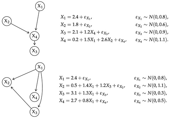
(Composing and decomposing a GBN). Consider the GBN from Figure 1 top. The topological ordering of the variables defined by is , so
where the diagonal elements are
and the elements below the diagonal are taken from the corresponding cells of
Computing gives
and reordering the rows and columns of gives
The elements of the corresponding expectation vector are then
Figure 1.
DAGs and local distributions for the GBNs (top) and (bottom) used in Examples 2 and 6–9.
Starting from , we can reorder its rows and columns to obtain . The Cholesky decomposition of is . Then
The coefficients of the local distributions are available from
where we can read , , .
We can read the standard errors of , , and directly from the diagonal elements of , and we can compute the intercepts from which amounts to
3.3. Conditional Linear Gaussian BNs
Finally, conditional linear Gaussian BNs [37] (CLGBNs) subsume discrete BNs and GBNs as particular cases by combining discrete and continuous random variables in a mixture model. If we denote the former with and the latter with , so that , then:
- Discrete are only allowed to have discrete parents (denoted ), and are assumed to follow a multinomial distribution parameterised with CPTs. We can estimate their parameters in the same way as those in a discrete BN.
- Continuous are allowed to have both discrete and continuous parents (denoted , ). Their local distributions arewhich is equivalent to a mixture of linear regressions against the continuous parents with one component for each configuration of the discrete parents:If has no discrete parents, the mixture reverts to a single linear regression like that in (4). The parameters of these local distributions are usually estimated by maximum likelihood like those in a GBN; we have used hierarchical regressions with random effects in our recent work [38] for this purpose as well. Bayesian and regularised estimators are also an option [5].
If the CLGBN comprises discrete nodes and continuous nodes, these distributional assumptions imply the partial topological ordering
The discrete nodes jointly follow a multinomial distribution, effectively forming a discrete BN. The continuous nodes jointly follow a multivariate normal distribution, parameterised as a GBN, for each configuration of the discrete nodes. Therefore, the global distribution is a Gaussian mixture in which the discrete nodes identify the components, and the continuous nodes determine their distribution. The practical link between the global and local distributions follows directly from Section 3.1 and Section 3.2.
Example 3
(Composing and decomposing a CLGBN). For reasons of space, this example is presented as Example A2 in Appendix B.
The complexity of composing and decomposing the global distribution is then
where are the discrete parents of the continuous nodes.
3.4. Inference
For BNs, inference broadly denotes obtaining the conditional distribution of a subset of variables conditional on a second subset of variables. Following older terminology from expert systems [2], this is called formulating a query in which we ask the BN about the probability of an event of interest after observing some evidence. In conditional probability queries, the event of interest is the probability of one or more events in (or the whole distribution of) some variables of interest conditional on the values assumed by the evidence variables. In maximum a posteriori (“most probable explanation”) queries, we condition the values of the evidence variables to predict those of the event variables.
All inference computations on BNs are completely automated by exact and approximate algorithms, which we will briefly describe here. We refer the interested reader to the more detailed treatment in Castillo et al. [2] and Koller and Friedman [5].
Exact inference algorithms use local computations to compute the value of the query. The seminal works of Lauritzen and Spiegelhalter [39], Lauritzen and Wermuth [37] and Lauritzen and Jensen [40] describe how to transform a discrete BN or a (CL)GBN into a junction tree as a preliminary step before using belief propagation. Cowell [41] uses elimination trees for the same purpose in CLGBNs. (A junction tree is an undirected tree whose nodes are the cliques in the moral graph constructed from the BN and their intersections. A clique is the maximal subset of nodes such that every two nodes in the subset are adjacent).
Namasivayam et al. [42] give the computational complexity of constructing the junction tree from a discrete BN as where w is the maximum number of nodes in a clique and, as before, l is the maximum number of values that a variable can take. We take the complexity of belief propagation to be , as stated in Lauritzen and Spiegelhalter [39] (“The global propagation is no worse than the initialisation [of the junction tree]”). This is confirmed by Pennock [43] and Namasivayam and Prasanna [44].
As for GBNs, we can also perform exact inference through their global distribution because the latter has only parameters. The computational complexity of this approach is because of the cost of composing the global distribution, which we derived in Section 3.2. However, all the operations involved are linear, making it possible to leverage specialised hardware such as GPUs and TPUs to the best effect. Koller and Friedman [5] (Section 14.2.1) note that “inference in linear Gaussian networks is linear in the number of cliques, and at most cubic in the size of the largest clique” when using junction trees and belief propagation. Therefore, junction trees may be significantly faster for GBNs when . However, the correctness and convergence of belief propagation in GBNs require a set of sufficient conditions that have been studied comprehensively by Malioutov et al. [45]. Using the global distribution directly always produces correct results.
Approximate inference algorithms use Monte Carlo simulations to sample from the global distribution of through the local distributions and estimate the answer queries by computing the appropriate summary statistics on the particles they generate. Therefore, they mirror the Monte Carlo and Markov chain Monte Carlo approaches in the literature: rejection sampling, importance sampling, and sequential Monte Carlo among others. Two state-of-the-art examples are the adaptive importance sampling (AIS-BN) scheme [46] and the evidence pre-propagation importance sampling (EPIS-BN) [47].
4. Shannon Entropy and Kullback–Leibler Divergence
The general definition of Shannon entropy for the probability distribution P of is
The Kullback–Leibler divergence between two distributions P and Q for the same random variables is defined as
They are linked as follows:
where is the cross-entropy between and . For the many properties of these quantities, we refer the reader to Cover and Thomas [48] and Csiszár and Shields [49]. Their use and interpretation are covered in depth (and breadth!) in Murphy [19,20] for general machine learning and in Koller and Friedman [5] for BNs.
For a BN encoding the probability distribution of , (6) decomposes into
where are the parents of in . While this decomposition looks similar to (1), we see that its terms are not necessarily orthogonal, unlike the local distributions.
As for (7), we cannot simply write
because, in the general case, the nodes have different parents in and . This issue impacts the complexity of computing Kullback–Leibler divergences in different ways depending on the type of BN.
4.1. Discrete BNs
For discrete BNs, does not decompose into orthogonal components. As pointed out in Koller and Friedman [5] (Section 8.4.12),
If we estimated the conditional probabilities from data, the are already available as the normalising constants of the individual conditional distributions in the local distribution of . In this case, the complexity of computing is linear in the number of parameters: .
In the general case, we need exact inference to compute the probabilities . Fortunately, they can be readily extracted from the junction tree derived from as follows:
- Identify a clique containing both and . Such a clique is guaranteed to exist by the family preservation property [5] (Definition 10.1).
- Compute the marginal distribution of by summing over the remaining variables in the clique.
Combining the computational complexity of constructing the junction tree from Section 3.4 and that of marginalisation, which is at most for each node as in (2), we have
which is exponential in the maximum clique size w. (The maximum clique size in a junction tree is proportional to the treewidth of the BN the junction tree is created from, which is also used in the literature to characterise computational complexity in BNs.) Interestingly, we do not need to perform belief propagation, so computing is more efficient than other inference tasks.
Example 4
(Entropy of a discrete BN). For reasons of space, this example is presented as Example A3 in Appendix B.
The Kullback–Leibler divergence has a similar issue, as noted in Koller and Friedman [5] (Section 8.4.2). The best and most complete explanation of how to compute it for discrete BNs is in Moral et al. [21]. After decomposing following (8) to separate and , Moral et al. [21] show that the latter takes the form
where:
- is the probability assigned by to given that the variables that are parents of in take value j;
- is the element of the CPT of in .
In order to compute the , we need to transform into its junction tree and use belief propagation to compute the joint distribution of . As a result, does not decompose at all: each can potentially depend on the whole BN .
Algorithmically, to compute we:
- Transform into its junction tree.
- Compute the entropy .
- For each node :
- (a)
- Identify , the parents of in .
- (b)
- Obtain the distribution of the variables from the junction tree of , consisting of the probabilities .
- (c)
- Read the from the local distribution of in .
- Use the and the to compute (10).
The computational complexity of this procedure is as follows:
As noted in Moral et al. [21], computing the requires a separate run of belief propagation for each configuration of the , for a total of times. If we assume that the DAG underlying is sparse, we have that and the overall complexity of this step becomes , N times that listed in Section 3.4. The caching scheme devised by Moral et al. [21] is very effective in limiting the use of belief propagation, but it does not alter its exponential complexity.
Example 5
Since both global distributions are limited in size, we can then compute the Kullback–Leibler divergence between and using (7).
In the general case, when we cannot use the global distributions, we follow the approach described in Section 4.1. Firstly, we apply (8) to write
we have from Example A3 that . As for the cross-entropy , we apply (10):
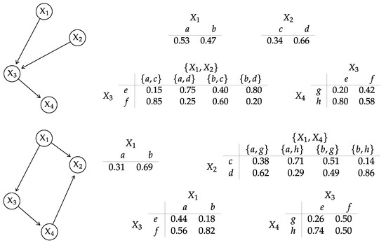
(KL between two discrete BNs). Consider the discrete BN from Figure 2 top. Furthermore, consider the BN from Figure 2 bottom. We constructed the global distribution of in Example A1; we can similarly compose the global distribution of , shown below.
Figure 2.
DAGs and local distributions for the discrete BNs (top) and (bottom) used in Examples 1, 4 and 5.
| e | f | e | f | e | f | e | f | |||||||
| g | g | g | g | |||||||||||
| h | h | h | h | |||||||||||
- 1.
- We identify the parents of each node in :
- 2.
- We construct a junction tree from and we use it to compute the distributions , , and .
a b c d a b e f e f g h - 3.
- We compute the cross-entropy terms for the individual variables in and :which sum up to .
- 4.
- We compute , which matches the value we previously computed from the global distributions.
4.2. Gaussian BNs
decomposes along with the local distributions in the case of GBNs: from (3), each is a univariate normal with variance and therefore
which has a computational complexity of O(1) for each node, O(N) overall. Equivalently, we can start from the global distribution of from Section 3.2 and consider that
because is lower triangular. The (multivariate normal) entropy of then becomes
in agreement with (12).
Example 6
(Entropy of a GBN). For reasons of space, this example is presented as Example A4 in Appendix B.
In the literature, the Kullback–Leibler divergence between two GBNs and is usually computed using the respective global distributions and [50,51,52]. The general expression is
which has computational complexity
The spectral decomposition gives the eigenvalues to compute and efficiently as illustrated in the example below. (Further computing the spectral decomposition of to compute from the eigenvalues does not improve complexity because it just replaces a single operation with another one.) We thus somewhat improve the overall complexity of to .
Example 7
(General-case KL between two GBNs). Consider the GBN Figure 1 top, which we know has global distribution
from Example 2. Furthermore, consider the GBN from Figure 1 bottom, which has global distribution
In order to compute , we first invert to obtain
which we then multiply by to compute the trace . We also use to compute . Finally, , and therefore
As an alternative, we can compute the spectral decompositions and as an intermediate step. Multiplying the sets of eigenvalues
gives the corresponding determinants; and it allows us to easily compute
for use in both the quadratic form and in the trace.
However, computing from the global distributions and disregards the fact that BNs are sparse models that can be characterised more compactly by and as shown in Section 3.2. In particular, we can revisit several operations that are in the high-order terms of (15):
- Composing the global distribution from the local ones. We avoid computing and , thus reducing this step to complexity.
- Computing the trace . We can reduce the computation of the trace as follows.
- We can replace and in the trace with any reordered matrix [53] (Result 8.17): we choose to use and where is defined as before and is with the rows and columns reordered to match . Formally, this is equivalent to where P is a permutation matrix that imposes the desired node ordering: since both the rows and the columns are permuted in the same way, the diagonal elements of are the same as those of and the trace is unaffected.
- We have .
- As for , we can write where is the lower triangular matrix with the rows re-ordered to match . Note that is not lower triangular unless and have the same partial node ordering, which implies .
Thereforewhere the last step rests on Seber [53] (Result 4.15). We can invert in time following Stewart [54] (Algorithm 2.3). Multiplying and is still . The Frobenius norm is since it is the sum of the squared elements of . - Computing the determinants and . From (13), each determinant can be computed in .
- Computing the quadratic term . Decomposing leads towhere and are the mean vectors re-ordered to match . The computational complexity is still because is available from previous computations.
The overall complexity of (19) KL is
while still cubic, the leading coefficient suggests that it should be about 5 times faster than the variant of (15) using the spectral decomposition.
Example 8
(Sparse KL between two GBNs). Consider again the two GBNs from Example 7. The corresponding matrices
readily give the determinants of and following (13):
As for the Frobenius norm in (17), we first invert to obtain
then we reorder the rows and columns of to follow the same node ordering as and compute
which, as expected, matches the value of we computed in Example 7. Finally, in (18) is
The quadratic form is then equal to , which matches the value of in Example 7. As a result, the expression for is the same as in (16).
We can further reduce the complexity (20) of (19) when an approximate value of KL is suitable for our purposes. The only term with cubic complexity is : reducing it to quadratic complexity or lower will eliminate the leading term of (20), making it quadratic in complexity. One way to do this is to compute a lower and an upper bound for , which can serve as an interval estimate, and take their geometric mean as an approximate point estimate.
A lower bound is given by Seber [53] (Result 10.39):
which conveniently reuses the values of and we have from (13). For an upper bound, Seber [53] (Result 10.59) combined with Seber [53] (Result 4.15) gives
a function of and that can be computed in time. Note that, as far as the point estimate is concerned, we do not care about how wide the interval is: we only need its geometric mean to be an acceptable approximation of .
Example 9
If we are comparing two GBNs whose parameters (but not necessarily network structures) have been learned from the same data, we can sometimes approximate using the local distributions and directly. If and have compatible partial orderings, we can define a common total node ordering for both such that
By “compatible partial orderings”, we mean two partial orderings that can be sorted into at least one shared total node ordering that is compatible with both. The product of the local distributions in the second step is obtained from the chain decomposition in the first step by considering the nodes in the conditioning other than the parents to have associated regression coefficients equal to zero. Then, following the derivations in Cavanaugh [55] for a general linear regression model, we can write the empirical approximation
where, following a similar notation to (4):
- , , , are the estimated intercepts and regression coefficients;
- and are the vectorsthe fitted values computed from the data observed for , , ;
- and are the residual variances in and .
We can compute the expression in (23) for each node in
which is linear in the sample size if both and are sparse because , . In this case, the overall computational complexity simplifies to . Furthermore, as we pointed out in Scutari et al. [29], the fitted values , are computed as a by-product of parameter learning: if we consider them to be already available, the above computational complexity is reduced to just O(n) for a single node and overall. We can also replace the fitted values , in (23) with the corresponding residuals , because
if the latter are available but the former are not.
Example 10
(KL between GBNs with parameters estimated from data). For reasons of space, this example is presented as Example A5 in Appendix B.
4.3. Conditional Gaussian BNs
The entropy decomposes into a separate for each node, of the form (9) for discrete nodes and (12) for continuous nodes with no discrete parents. For continuous nodes with both discrete and continuous parents,
where represents the probability associated with the configuration of the discrete parents . This last expression can be computed in time for each node. Overall, the complexity of computing is
where the max accounts for the fact that when but the computational complexity is O(1) for such nodes.
Example 11
(Entropy of a CLGBN). For reasons of space, this example is presented as Example A6 in Appendix B.
As for , we could not find any literature illustrating how to compute it. The partition of the nodes in (5) implies that
We can compute the first term following Section 4.1: and form two discrete BNs whose DAGs are the spanning subgraphs of and and whose local distributions are the corresponding ones in and , respectively. The second term decomposes into
similarly to (10) and (24). We can compute it using the multivariate normal distributions associated with the and the in the global distributions of and .
Example 12
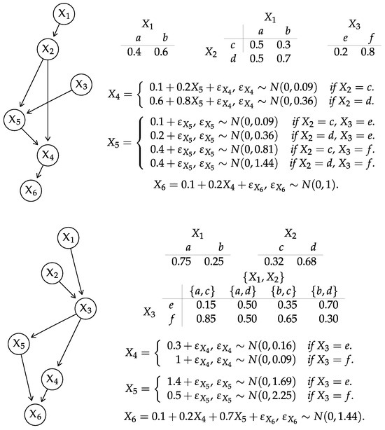
(General-case KL between two CLGBNs). Consider the CLGBNs from Figure 3 top, which we already used in Examples 3 and 11, and from Figure 3 bottom. The variables identify the following mixture components in the global distribution of :
Therefore, only encodes two different multivariate normal distributions.
Figure 3.
DAGs and local distributions for the CLGBNs (top) and (bottom) used in Examples 3 and 11–13.
Firstly, we construct two discrete BNs using the subgraphs spanning in and , which have arcs and , respectively. The CPTs for , and are the same as in and in . We then compute following Example 5.
Secondly, we construct the multivariate normal distributions associated with the components of following Example 3 (in which we computed those of ). For , we have
for , we have
Then,
and .
The computational complexity of this basic approach to computing is
which we obtain by adapting (11) and (15) to follow the notation and we established in Section 3.3. The first term implicitly covers the cost of computing the , which relies on exact inference like the computation of . The second term is exponential in M, which would lead us to conclude that it is computationally unfeasible to compute whenever we have more than a few discrete variables in and . Certainly, this would agree with Hershey and Olsen [22], who reviewed various scalable approximations of the KL divergence between two Gaussian mixtures.
However, we would again disregard the fact that BNs are sparse models. Two properties of CLGBNs that are apparent from Examples 3 and 12 allow us to compute (26) efficiently:
- We can reduce to where . In other words, the continuous nodes are conditionally independent on the discrete nodes that are not their parents () given their parents (). The same is true for . The number of distinct terms in the summation in (26) is then given by which will be smaller than in sparse networks.
- The conditional distributions and are multivariate normals (not mixtures). They are also faithful to the subgraphs spanning the continuous nodes , and we can represent them as GBNs whose parameters can be extracted directly from and . Therefore, we can use the results from Section 4.2 to compute their Kullback–Leibler divergences efficiently.
As a result, (26) simplifies to
where is the probability that the nodes take value as computed in . In turn, (27) reduces to
because we can replace with , which is an upper bound to the unique components in the mixture, and because we replace the complexity in (15) with that (20). We can also further reduce the second term to quadratic complexity as we discussed in Section 4.2. The remaining drivers of the computational complexity are:
- the maximum clique size w in the subgraph spanning ;
- the number of arcs from discrete nodes to continuous nodes in both and and the overlap between and .
Example 13
(Sparse KL between two CLGBNs). Consider again the CLGBNs and from Example 12. The node sets and identify four KL divergences to compute: .
All the BNs in the Kullback–Leibler divergences are GBNs whose structure and local distributions can be read from and . The four GBNs associated with have nodes , arcs and the local distributions listed in Figure 3. The corresponding GBNs associated with are, in fact, only two distinct GBNs associated with and . They have arcs and local distributions: for ,
for ,
Plugging in the numbers,
which matches the value we computed in Example 12.
5. Conclusions
We started this paper by reviewing the three most common distributional assumptions for BNs: discrete BNs, Gaussian BNs (GBNs) and conditional linear Gaussian BNs (CLGBNs). Firstly, we reviewed the link between the respective global and local distributions, and we formalised the computational complexity of decomposing the former into the latter (and vice versa).
We then leveraged these results to study the complexity of computing Shannon’s entropy. We can, of course, compute the entropy of a BN from its global distribution using standard results from the literature. (In the case of discrete BNs and CLGBNS, only for small networks because grows combinatorially.) However, this is not computationally efficient because we incur the cost of composing the global distribution. While the entropy does not decompose along with the local distributions for either discrete BNs or CLGBNS, we show that it is nevertheless efficient to compute it from them.
Computing the Kullback–Leibler divergence between two BNs following the little material found in the literature is more demanding. The discrete case has been thoroughly investigated by Moral et al. [21]. However, the literature typically relies on composing the global distributions for GBNs and CGBNs. Using the local distributions, thus leveraging the intrinsic sparsity of BNs, we showed how to compute the Kullback–Leibler divergence exactly with greater efficiency. For GBNs, we showed how to compute the Kullback–Leibler divergence approximately with quadratic complexity (instead of cubic). If the two GBNs have compatible node orderings and their parameters are estimated from the same data, we can also approximate their Kullback–Leibler divergence with complexity that scales with the number of parents of each node. All these results are summarised in Table A1 in Appendix A.
Finally, we provided step-by-step numeric examples of how to compute Shannon’s entropy and the Kullback–Leibler divergence for discrete BNs, GBNs and CLGBNs. (See also Appendix B). Considering this is a highly technical topic, and no such examples are available anywhere in the literature, we feel that they are helpful in demystifying this topic and in integrating BNs into many general machine learning approaches.
Funding
This research received no external funding.
Data Availability Statement
Data are contained within the article.
Conflicts of Interest
The author declares no conflict of interest.
Appendix A. Computational Complexity Results
For ease of reference, we summarise here all the computational complexity results in this paper, including the type of BN and the page where they have been derived.

Table A1.
Summary of all the computational complexity results in this paper, including the type of BN and the page where they have been derived.
Table A1.
Summary of all the computational complexity results in this paper, including the type of BN and the page where they have been derived.
| Composing and decomposing the global distributions | ||
| discrete BNs | Section 3.1 | |
| GBNs | Section 3.2 | |
| CLGBNs | Section 3.3 | |
| Computing Shannon’s entropy | ||
| discrete BNs | Section 4.1 | |
| O(N) | GBNs | Section 4.2 |
| CLGBNs | Section 4.3 | |
| Computing the Kullback–Leibler divergence | ||
| discrete BNs | Section 4.1 | |
| GBNs | Section 4.2 | |
| CLGBNs | Section 4.3 | |
| Sparse Kullback–Leibler divergence | ||
| GBNs | Section 4.2 | |
| CLGBNs | Section 4.3 | |
| Approximate Kullback–Leibler divergence | ||
| GBNs | Section 4.2 | |
| Efficient empirical Kullback–Leibler divergence | ||
| GBNs | Section 4.2 | |
Appendix B. Additional Examples
Example A1
The joint probabilities are computed by multiplying the appropriate cells of the CPTs, for instance
(Composing and decomposing a discrete BN). Consider the discrete BN shown in Figure 2 (top). Composing its global distribution entails computing the joint probabilities of all possible states of all variables,
and arranging them in the following four-dimensional probability table in which each dimension is associated with one of the variables.
| e | f | e | f | e | f | e | f | |||||||
| g | g | g | g | |||||||||||
| h | h | h | h | |||||||||||
Conversely, we can decompose the global distribution into the local distributions by summing over all variables other than the nodes and their parents. For , this means
Similarly, for we obtain
For , we first compute the joint distribution of and by marginalising over and ,
from which we obtain the CPT for by normalising its columns.
As for , we marginalise over to obtain the joint distribution of , and
and we obtain the CPT for by normalising its columns as we did earlier with .
Example A2
(Composing and decomposing a CLGBN). Consider the CLGBN from Figure 3 top. The discrete variables at the top of the network have the joint distribution below:
Its elements identify the components of the mixture that make up the global distribution of , and the associated probabilities are the probabilities of those components.
We can then identify which parts of the local distributions of the continuous variables (, and ) we need to compute for each element of the mixture. The graphical structure of implies that because the continuous nodes are d-separated from by their parents. As a result, the following mixture components will share identical distributions which only depend on the configurations of and :
For the mixture components with a distribution identified by , the relevant parts of the distributions of , and are:
We can treat them as the local distributions in a GBN over with a DAG equal to the subgraph of spanning only these nodes. If we follow the steps outlined in Section 3.2 and illustrated in Example 2, we obtain
which is the multivariate normal distribution associated with the components and in the mixture. Similarly, the relevant parts of the distributions of , and for are
and jointly
for the components and . For the components and , the local distributions identified by are
and the joint distribution of , and is
Finally, the local distributions identified by are
and the joint distribution of , and for the components , is
We follow the same steps in reverse to decompose the global distribution into the local distributions. The joint distribution of is a mixture with multivariate normal components and the associated probabilities. The latter are a function of the discrete variables , , : rearranging them as the three-dimensional table
gives us the typical representation of , which we can work with by operating over the different dimensions. We can then compute the conditional probability tables in the local distributions of and by marginalising over the remaining variables:
As for , we marginalise over and normalise over to obtain
The multivariate normal distributions associated with the mixture components are a function of the continuous variables , , . has only one discrete parent (), has two ( and ) and has none. Therefore, we only need to examine four mixture components to obtain the parameters of the local distributions of all three variables: one for which , one for which , one for which and one for which .
|
| ||||||||||||||||||||||||||||||||||||||||
If we consider the first mixture component , we can apply the steps described Section 3.2 to decompose it into the local distributions of , , and obtain
Similarly, the third mixture component yields
The fifth mixture component yields
The seventh mixture component yields
Reorganising these distributions by variables we obtain the local distributions of shown in Figure 3 top.
Example A3
(Entropy of a discrete BN). Consider again the discrete BN from Example A1. In this simple example, we can use its global distribution and (6) to compute
In the general case, we compute from the local distributions using (9). Since and have no parents, their entropy components simply sum over their marginal distributions:
For ,
where
and where (multiplying the marginal probabilities for and , which are marginally independent)
giving
Finally, for
where
and , , giving
Combining all these figures, we obtain as
as before.
In general, we would have to compute the probabilities of the parent configurations of each node using a junction tree as follows:
- 1.
- We construct the moral graph of , which contains the same arcs (but undirected) as its DAG plus .
- 2.
- We identify two cliques and and a separator .
- 3.
- We connect them to create the junction tree .
- 4.
- We initialise the cliques with the respective distributions , and .
- 5.
- We compute and .
Example A4
Example A5
(KL between GBNs with parameters estimated from data). Consider the DAGs for the BNs and and the 10 observations shown in Figure A1. The partial topological ordering of the nodes in is and that in is : the total ordering that is compatible with both is .
If we estimate the parameters of the local distributions of by maximum likelihood we obtain
and the associated fitted values are
Similarly, for we obtain
and the associated fitted values are
Therefore,
and the values of the Kullback–Leibler divergence for the individual nodes are
which sum up to . The exact value, which we can compute as shown in Section 4.2, is .
The quality of the empirical approximation improves with the number of observations. For reference, we generated the data in Figure A1 from the GBN in Example 2. With a sample of size from the same network, with ; with , with .
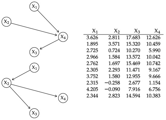
Figure A1.
The DAGs for the GBNs (top left) and (bottom left) and the data (right) used in Example A5.
Example A6
(Entropy of a CLGBN). Consider again the CLGBN from from Figure 3 (top). For such a simple BN, we can use its global distribution (which we derived in Example A2) directly to compute the entropies of the multivariate normal distributions associated with the mixture components
and to combine them by weighting with the component probabilities
The entropy of the discrete variables is
and then .
If we use the local distributions instead, we can compute the entropy of the discrete variables using (9) from Section 4.1:
We can compute the entropy of the continuous variables with no discrete parents using (12) from Section 4.2:
Finally, we can compute the entropy of the continuous variables with discrete parents using (24) from Section 4.3:
As before, we confirm that overall
References
- Scutari, M.; Denis, J.B. Bayesian Networks with Examples in R, 2nd ed.; Chapman & Hall: Boca Raton, FL, USA, 2021. [Google Scholar]
- Castillo, E.; Gutiérrez, J.M.; Hadi, A.S. Expert Systems and Probabilistic Network Models; Springer: Berlin/Heidelberg, Germany, 1997. [Google Scholar]
- Cowell, R.G.; Dawid, A.P.; Lauritzen, S.L.; Spiegelhalter, D.J. Probabilistic Networks and Expert Systems; Springer: Berlin/Heidelberg, Germany, 1999. [Google Scholar]
- Pearl, J. Probabilistic Reasoning in Intelligent Systems: Networks of Plausible Inference; Morgan Kaufmann: Burlington, MA, USA, 1988. [Google Scholar]
- Koller, D.; Friedman, N. Probabilistic Graphical Models: Principles and Techniques; MIT Press: Cambridge, MA, USA, 2009. [Google Scholar]
- Murphy, K.P. Dynamic Bayesian Networks: Representation, Inference and Learning. Ph.D. Thesis, Computer Science Division, UC Berkeley, Berkeley, CA, USA, 2002. [Google Scholar]
- Spirtes, P.; Glymour, C.; Scheines, R. Causation, Prediction, and Search; MIT Press: Cambridge, MA, USA, 2000. [Google Scholar]
- Pearl, J. Causality: Models, Reasoning and Inference, 2nd ed.; Cambridge University Press: Cambridge, UK, 2009. [Google Scholar]
- Borsboom, D.; Deserno, M.K.; Rhemtulla, M.; Epskamp, S.; Fried, E.I.; McNally, R.J.; Robinaugh, D.J.; Perugini, M.; Dalege, J.; Costantini, G.; et al. Network Analysis of Multivariate Data in Psychological Science. Nat. Rev. Methods Prim. 2021, 1, 58. [Google Scholar]
- Carapito, R.; Li, R.; Helms, J.; Carapito, C.; Gujja, S.; Rolli, V.; Guimaraes, R.; Malagon-Lopez, J.; Spinnhirny, P.; Lederle, A.; et al. Identification of Driver Genes for Critical Forms of COVID-19 in a Deeply Phenotyped Young Patient Cohort. Sci. Transl. Med. 2021, 14, 1–20. [Google Scholar]
- Requejo-Castro, D.; Giné-Garriga, R.; Pérez-Foguet, A. Data-driven Bayesian Network Modelling to Explore the Relationships Between SDG 6 and the 2030 Agenda. Sci. Total Environ. 2020, 710, 136014. [Google Scholar] [PubMed]
- Zilko, A.A.; Kurowicka, D.; Goverde, R.M.P. Modeling Railway Disruption Lengths with Copula Bayesian Networks. Transp. Res. Part C Emerg. Technol. 2016, 68, 350–368. [Google Scholar]
- Gao, R.X.; Wang, L.; Helu, M.; Teti, R. Big Data Analytics for Smart Factories of the Future. CIRP Ann. 2020, 69, 668–692. [Google Scholar]
- Blei, D.M.; Kucukelbir, A.; McAuliffe, J.D. Variational Inference: A Review for Statisticians. J. Am. Stat. Assoc. 2017, 112, 859–877. [Google Scholar]
- Dempster, A.P.; Laird, N.M.; Rubin, D.B. Maximum Likelihood From Incomplete Data via the EM Algorithm. J. R. Stat. Soc. (Ser. B) 1977, 39, 1–22. [Google Scholar] [CrossRef]
- Minka, T.P. Expectation Propagation for Approximate Bayesian Inference. In Proceedings of the 17th Conference on Uncertainty in Artificial Intelligence (UAI), Seattle, WA, USA, 2–5 August 2001; pp. 362–369. [Google Scholar]
- van der Maaten, L.; Hinton, G. Visualizing Data Using t-SNE. J. Mach. Learn. Res. 2008, 9, 2579–3605. [Google Scholar]
- Becht, E.; McInnes, L.; Healy, J.; Dutertre, C.A.; Kwok, I.W.H.; Ng, L.G.; Ginhoux, F.; Newell, E.W. Dimensionality Reduction for Visualizing Single-Cell Data Using UMAP. Nat. Biotechnol. 2019, 37, 38–44. [Google Scholar] [CrossRef]
- Murphy, K.P. Probabilistic Machine Learning: An Introduction; MIT Press: Cambridge, MA, USA, 2022. [Google Scholar]
- Murphy, K.P. Probabilistic Machine Learning: Advanced Topics; MIT Press: Cambridge, MA, USA, 2023. [Google Scholar]
- Moral, S.; Cano, A.; Gómez-Olmedo, M. Computation of Kullback–Leibler Divergence in Bayesian Networks. Entropy 2021, 23, 1122. [Google Scholar] [CrossRef]
- Hershey, J.R.; Olsen, P.A. Approximating the Kullback Leibler Divergence Between Gaussian Mixture Models. In Proceedings of the 32nd IEEE International Conference on Acoustics, Speech and Signal Processing (ICASSP), Honolulu, HI, USA, 15–20 April 2007; Volume IV, pp. 317–320. [Google Scholar]
- Beskos, A.; Crisan, D.; Jasra, A. On the Stability of Sequential Monte Carlo Methods in High Dimensions. Ann. Appl. Probab. 2014, 24, 1396–1445. [Google Scholar] [CrossRef]
- Scutari, M. Learning Bayesian Networks with the bnlearn R Package. J. Stat. Softw. 2010, 35, 1–22. [Google Scholar] [CrossRef]
- Heckerman, D.; Geiger, D.; Chickering, D.M. Learning Bayesian Networks: The Combination of Knowledge and Statistical Data. Mach. Learn. 1995, 20, 197–243. [Google Scholar] [CrossRef]
- Chickering, D.M.; Heckerman, D. Learning Bayesian Networks is NP-Hard; Technical Report MSR-TR-94-17; Microsoft Corporation: Redmond, WA, USA, 1994. [Google Scholar]
- Chickering, D.M. Learning Bayesian Networks is NP-Complete. In Learning from Data: Artificial Intelligence and Statistics V; Fisher, D., Lenz, H., Eds.; Springer: Berlin/Heidelberg, Germany, 1996; pp. 121–130. [Google Scholar]
- Chickering, D.M.; Heckerman, D.; Meek, C. Large-sample Learning of Bayesian Networks is NP-hard. J. Mach. Learn. Res. 2004, 5, 1287–1330. [Google Scholar]
- Scutari, M.; Vitolo, C.; Tucker, A. Learning Bayesian Networks from Big Data with Greedy Search: Computational Complexity and Efficient Implementation. Stat. Comput. 2019, 25, 1095–1108. [Google Scholar] [CrossRef]
- Cussens, J. Bayesian Network Learning with Cutting Planes. In Proceedings of the 27th Conference on Uncertainty in Artificial Intelligence (UAI), Barcelona, Spain, 14–17 July 2011; pp. 153–160. [Google Scholar]
- Suzuki, J. An Efficient Bayesian Network Structure Learning Strategy. New Gener. Comput. 2017, 35, 105–124. [Google Scholar] [CrossRef]
- Scanagatta, M.; de Campos, C.P.; Corani, G.; Zaffalon, M. Learning Bayesian Networks with Thousands of Variables. Adv. Neural Inf. Process. Syst. (Nips) 2015, 28, 1864–1872. [Google Scholar]
- Hausser, J.; Strimmer, K. Entropy Inference and the James-Stein Estimator, with Application to Nonlinear Gene Association Networks. J. Mach. Learn. Res. 2009, 10, 1469–1484. [Google Scholar]
- Agresti, A. Categorical Data Analysis, 3rd ed.; Wiley: Hoboken, NJ, USA, 2012. [Google Scholar]
- Geiger, D.; Heckerman, D. Learning Gaussian Networks. In Proceedings of the 10th Conference on Uncertainty in Artificial Intelligence (UAI), Seattle, WA, USA, 29–31 July 1994; pp. 235–243. [Google Scholar]
- Pourahmadi, M. Covariance Estimation: The GLM and Regularization Perspectives. Stat. Sci. 2011, 26, 369–387. [Google Scholar]
- Lauritzen, S.L.; Wermuth, N. Graphical Models for Associations between Variables, Some of which are Qualitative and Some Quantitative. Ann. Stat. 1989, 17, 31–57. [Google Scholar] [CrossRef]
- Scutari, M.; Marquis, C.; Azzimonti, L. Using Mixed-Effect Models to Learn Bayesian Networks from Related Data Sets. In Proceedings of the International Conference on Probabilistic Graphical Models, Almería, Spain, 5–7 October 2022; Volume 186, pp. 73–84. [Google Scholar]
- Lauritzen, S.L.; Spiegelhalter, D.J. Local Computation with Probabilities on Graphical Structures and their Application to Expert Systems (with discussion). J. R. Stat. Soc. Ser. B (Stat. Methodol.) 1988, 50, 157–224. [Google Scholar]
- Lauritzen, S.L.; Jensen, F. Stable Local Computation with Conditional Gaussian Distributions. Stat. Comput. 2001, 11, 191–203. [Google Scholar] [CrossRef]
- Cowell, R.G. Local Propagation in Conditional Gaussian Bayesian Networks. J. Mach. Learn. Res. 2005, 6, 1517–1550. [Google Scholar]
- Namasivayam, V.K.; Pathak, A.; Prasanna, V.K. Scalable Parallel Implementation of Bayesian Network to Junction Tree Conversion for Exact Inference. In Proceedings of the 18th International Symposium on Computer Architecture and High Performance Computing, Ouro Preto, Brazil, 17–20 October 2006; pp. 167–176. [Google Scholar]
- Pennock, D.M. Logarithmic Time Parallel Bayesian Inference. In Proceedings of the 14th Conference on Uncertainty in Artificial Intelligence (UAI), Pittsburgh, PA, USA, 31 July–4 August 2023; pp. 431–438. [Google Scholar]
- Namasivayam, V.K.; Prasanna, V.K. Scalable Parallel Implementation of Exact Inference in Bayesian Networks. In Proceedings of the 12th International Conference on Parallel and Distributed Systems (ICPADS), Minneapolis, MN, USA, 12–15 July 2006; pp. 1–8. [Google Scholar]
- Malioutov, D.M.; Johnson, J.K.; Willsky, A.S. Walk-Sums and Belief Propagation in Gaussian Graphical Models. J. Mach. Learn. Res. 2006, 7, 2031–2064. [Google Scholar]
- Cheng, J.; Druzdzel, M.J. AIS-BN: An Adaptive Importance Sampling Algorithm for Evidential Reasoning in Large Bayesian Networks. J. Artif. Intell. Res. 2000, 13, 155–188. [Google Scholar] [CrossRef]
- Yuan, C.; Druzdzel, M.J. An Importance Sampling Algorithm Based on Evidence Pre-Propagation. In Proceedings of the 19th Conference on Uncertainty in Artificial Intelligence (UAI), Acapulco, Mexico, 7–10 August 2003; pp. 624–631. [Google Scholar]
- Cover, T.M.; Thomas, J.A. Elements of Information Theory, 2nd ed.; Wiley: Hoboken, NJ, USA, 2006. [Google Scholar]
- Csiszár, I.; Shields, P. Information Theory and Statistics: A Tutorial; Now Publishers Inc.: Delft, The Netherlands, 2004. [Google Scholar]
- Gómez-Villegas, M.A.; Main, P.; Susi, R. Sensitivity of Gaussian Bayesian Networks to Inaccuracies in Their Parameters. In Proceedings of the 4th European Workshop on Probabilistic Graphical Models (PGM), Cuenca, Spain, 17–19 September 2008; pp. 265–272. [Google Scholar]
- Gómez-Villegas, M.A.; Main, P.; Susi, R. The Effect of Block Parameter Perturbations in Gaussian Bayesian Networks: Sensitivity and Robustness. Inf. Sci. 2013, 222, 439–458. [Google Scholar] [CrossRef]
- Görgen, C.; Leonelli, M. Model-Preserving Sensitivity Analysis for Families of Gaussian Distributions. J. Mach. Learn. Res. 2020, 21, 1–32. [Google Scholar]
- Seber, G.A.F. A Matrix Handbook for Stasticians; Wiley: Hoboken, NJ, USA, 2008. [Google Scholar]
- Stewart, G.W. Matrix Algorithms, Volume I: Basic Decompositions; SIAM: Philadelphia, PA, USA, 1998. [Google Scholar]
- Cavanaugh, J.E. Criteria for Linear Model Selection Based on Kullback’s Symmetric Divergence. Aust. N. Z. J. Stat. 2004, 46, 197–323. [Google Scholar] [CrossRef]
Disclaimer/Publisher’s Note: The statements, opinions and data contained in all publications are solely those of the individual author(s) and contributor(s) and not of MDPI and/or the editor(s). MDPI and/or the editor(s) disclaim responsibility for any injury to people or property resulting from any ideas, methods, instructions or products referred to in the content. |
© 2024 by the author. Licensee MDPI, Basel, Switzerland. This article is an open access article distributed under the terms and conditions of the Creative Commons Attribution (CC BY) license (https://creativecommons.org/licenses/by/4.0/).