Algorithms for Fractional Dynamical Behaviors Modelling Using Non-Singular Rational Kernels

Abstract

This paper proposes algorithms to model fractional (dynamical) behaviors using non-singular rational kernels whose interest is first demonstrated on a pure power law function. Two algorithms are then proposed to find a non-singular rational kernel that allows the input-output data to be fitted. The first one derives the impulse response of the modeled system from the data. The second one finds the interlaced poles and zeros of the rational function that fits the impulse response found using the first algorithm. Several applications show the efficiency of the proposed work.

1. Introduction

The search for non-singular kernels [1,2,3,4,5] or alternative solutions to fractional models [6,7] is gaining momentum in the field of modeling fractional dynamical behaviors. Using such kernels makes it possible to overcome certain limitations of fractional models, such as fractional differential equations or pseudo-state space descriptions, which have recently been highlighted [8,9,10,11,12,13,14]. For instance, it was demonstrated that a fractional integrator operator in the Riemann–Liouville sense [15,16] involves infinitely large and infinitely small time constants, which makes fractional models doubly infinite models: infinite because distributed, but also infinite as defined on an infinite equivalent spatial domain [17]. In a modelling context, these infinitely large and infinitely small time constants are not required to capture the behavior of a real system that operates on finite spatial and time scales. Moreover, these time constants introduced by fractional models (and that do exist in the modelled system) can greatly complicate the analyses and lead to erroneous conclusions on certain internal properties of the modelled system. This is the case for initialization [18,19] or observability for example [20].

However, fractional behaviors (produced by physical phenomena) and fractional models should be distinguished. The former designates a property of a physical system while the latter designates a model class, among a set of model classes able to capture fractional dynamical behaviors. Based on this observation, a whole new field opens up, from the search for new models dedicated to capturing fractional behaviors to the study of their properties and the development of identification methods. A few studies undertaken from this perspective are already available in the literature [6,7], which is also the case in the present article.

To overcome the limitations mentioned in the first paragraph, we propose in this paper to use non-singular rational kernels to model fractional behaviors and propose an algorithm to find the parameters in the kernel description. Non-singular rational kernels are considered for the three following reasons:

-

a fractional behavior defined by the power law $t^{-\nu }$, can be associated with a rational function with an infinite number of interlaced poles and zeros as shown in this paper.

-

the approximation of such a function by rational functions of degree $n$ leads to a very small approximation error in comparison to polynomials of degree $n$ [21];

-

rational kernels permit the approximation of fractional behaviors with a reduced number of parameters in comparison to fractional models.

For all these reasons, it appeared necessary to develop a simple and efficient algorithm allowing the determination of the coefficients of a rational kernel in a convolution model, which fits a given fractional behavior with a defined given level of accuracy.

To the best knowledge of the authors, there is no method that allows a direct estimation of the parameters of a rational kernel in a convolution model. That is why we have defined a two-step method that consists of:

-

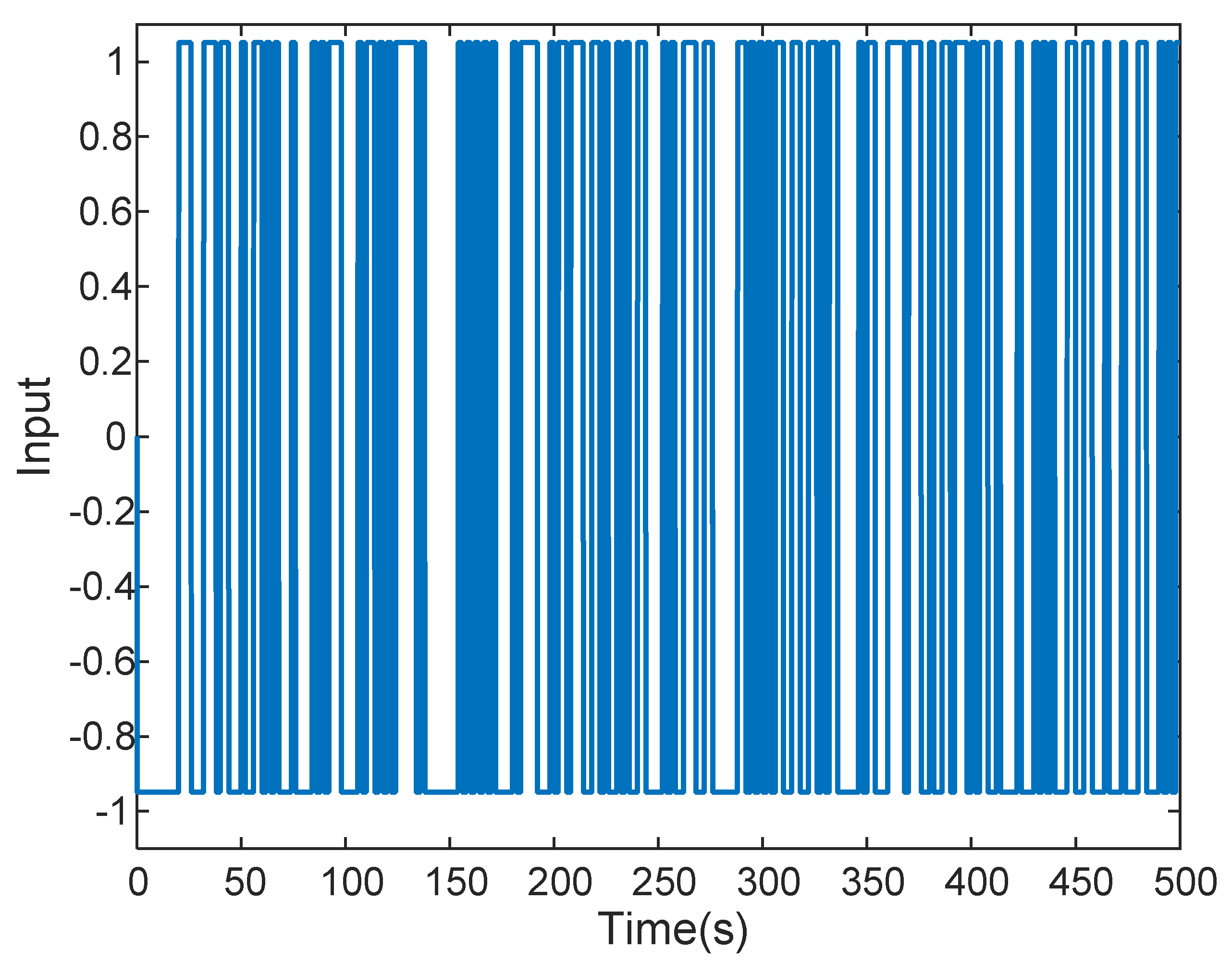
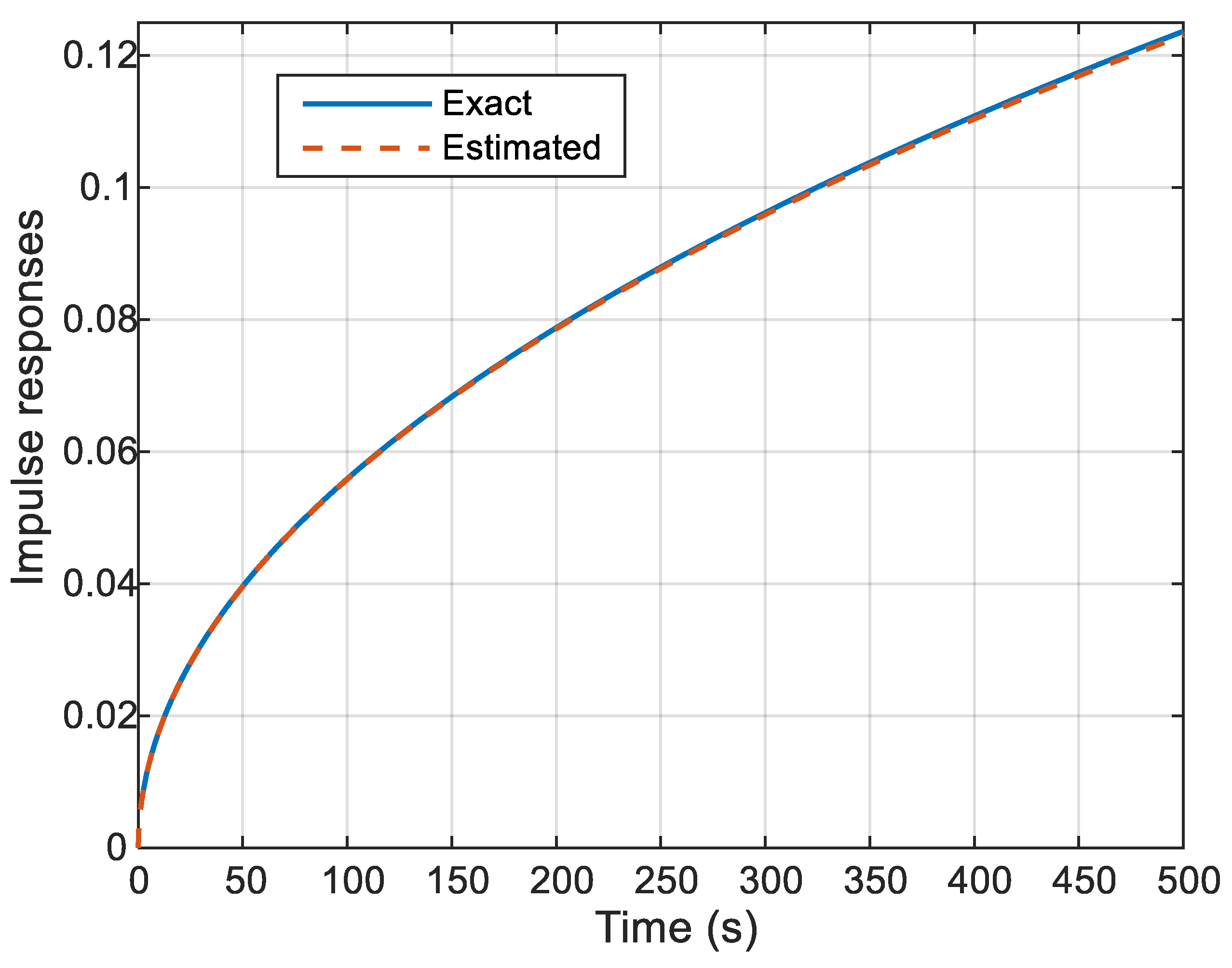
first, estimating the time response of the kernel in the convolution model that fits the input-output behavior of the modeled system.

-

then, estimate the parameters of a rational function that fits the kernel time response.

For the second step of this strategy, there are many methods that allow rational interpolation [22,23,24,25,26]. But these methods are not well adapted to fractional behaviors, that is to say with time behaviors with slow convergence. On the other hand, when working in the logarithmic domain as in the methodology we propose, a time compression occurs which facilitates fitting over large time domains.

The paper is thus organized as follows. In Section 2, the approximation of a pure power law function $K{t}^{-\nu }$ by a rational function involving interlaced poles and zeros is considered. It demonstrates the accuracy and the simplicity of rational kernels to approximate a fractional behavior and thus justifies their use. In Section 3, two algorithms are proposed to find a non-singular rational kernel capable of fitting input-output data. The first one derives the impulse response of a system from the data. The second one finds the interlaced poles and zeros of the rational function that is used to fit the impulse response found in the first step. Several applications are presented in Section 4 to show the efficiency of the proposed algorithms.

2. Approximation of a Pure Power Law Behavior by Non-Singular Rational Kernels

This section shows the efficiency of non-singular rational kernels for the modelling of fractional behaviors. The fractional behavior considered is first the pure power law function:

$${\eta }_{\nu }\left(t\right)=K{t}^{-\nu }$$

(1)

This function indeed falls within the definition of a fractional integration order operator defined in the Riemann–Liouville sense by [15,16]

$$I^{\gamma }\left[u\left(t\right)\right]=\frac{1}{\mathsf{\Gamma }\left(\gamma \right)}{\int }_0^t\frac{1}{{\left(t-\tau \right)}^{1-\gamma }}u\left(\tau \right)d\tau ={\eta }_{PL}\left(t\right)\ast u\left(t\right),$$

(2)

with ${\eta }_{PL}\left(t\right)=t^{\gamma -1}/\mathsf{\Gamma }\left(\gamma \right)$. The idea is to approximate the kernel ${\eta }_{PL}\left(t\right)$ by a non-singular rational kernel $\eta \left(t\right)$, to avoid the limitations cited in the introduction, while allowing the model

$$y\left(t\right)={\int }_0^t\eta \left(t-\tau \right)u\left(\tau \right)d\tau =\eta \left(t\right)\ast u\left(t\right),$$

(3)

to capture fractional behaviors.

For the approximation of ${\eta }_{\nu }\left(t\right)$, the following rational kernel is considered:

$$\eta \left(t\right)=C_0\frac{\prod _{j=1}^N\left(\frac{t}{t_j^{\prime }}+1\right)}{\prod _{j=1}^N\left(\frac{t}{t_j}+1\right)}.$$

(4)

The decimal logarithm of $\eta \left(t\right)$ is

$$\log \left(\eta \left(t\right)\right)=\mathrm{l}\mathrm{o}\mathrm{g}\left(C_0\right)+{\sum }_{j=1}^N\log \left(\frac{t}{t_j^{\prime }}+1\right)-{\sum }_{j=1}^N\log \left(\frac{t}{t_j}+1\right)$$

(5)

Decimal logarithm applied to the function ${\eta }_{\nu }\left(t\right)$ gives:

$$\log \left({\eta }_{\nu }\left(t\right)\right)=\log \left(K\right)-\nu \log \left(t\right).$$

(6)

At $t=1$, from (1),

$${\eta }_{\nu }\left(1\right)=K$$

(7)

and using relation (4),

$$\eta \left(1\right)=C_0\frac{\prod _{j=1}^N\left(\frac{1}{t_j^{\prime }}+1\right)}{\prod _{j=1}^N\left(\frac{1}{t_j}+1\right)}.$$

(8)

Thus, to ensure that $\eta \left(1\right)={\eta }_{\nu }\left(1\right)$, it is imposed that

$$C_0=K\frac{\prod _{j=1}^N\left(\frac{1}{t_j}+1\right)}{\prod _{j=1}^N\left(\frac{1}{t_j^{\prime }}+1\right)}.$$

(9)

The functions ${\eta }_z\left(t\right)=\log \left(\frac{t}{t_j^{\prime }}+1\right)$ and ${\eta }_p\left(t\right)=-\log \left(\frac{t}{t_j}+1\right)$ of relation (5) are represented in Figure 1 for $t_j^{\prime }=t_j=1$, as a function of $\log \left(t\right)$. For $t>\left(t_j^{\prime }=1\right)$ and $t>\left(t_j=1\right)$, the functions ${\eta }_z\left(t\right)$ and ${\eta }_p\left(t\right)$ behave, respectively, as lines of slope 1 and −1. The function given by relation (2) has a slope of $–\nu$ on a logarithmic scale. Thus, taking inspiration from the work which aimed to approximate fractional integrator operators in the frequency domain [27,28,29,30,31,32], and adapting them to the time domain, the function ${\eta }_{\nu }\left(t\right)$ can be approximated by choosing the appropriate values of $t_j^{\prime }$ and $t_j$ in an alternation of function ${\eta }_p\left(t\right)$ and ${\eta }_z\left(t\right)$.

Figure 1. Representation of functions ${\eta }_z\left(t\right)=\log \left(\frac{t}{t_j^{\prime }}+1\right)$ and ${\eta }_p\left(t\right)=-\log \left(\frac{t}{t_j}+1\right)$ for $t_j^{\prime }=t_j=1$, as functions of $\log \left(t\right)$.

Figure 2 describes how the functions ${\eta }_z\left(t\right)$ and ${\eta }_p\left(t\right)$ are used to produce the desired slope. On this figure, it is assumed that an approximation of relation (1) is required on the time interval $\left[t_l,t_h\right]$. In the functions ${\eta }_z\left(t\right)$ and ${\eta }_p\left(t\right)$, it is assumed that the time $t_j^{\prime }$ and $t_j$ meet the following relations

$$\log \left(\alpha \right)=\log \left(t_j^{\prime }\right)-\log \left(t_j\right) \mathrm{and} \mathrm{thus} \alpha =\frac{t_j^{\prime }}{t_j}$$

(10)

$$\log \left(\eta \right)=\log \left(t_{j+1}\right)-\log \left(t_j^{\prime }\right) \mathrm{and} \mathrm{thus} \beta =\frac{t_{j+1}}{t_j^{\prime }}$$

(11)

$$\log \left(\alpha \right)+\log \left(\beta \right)=\log \left(t_{j+1}\right)-\log \left(t_j\right)=\log \left({t\prime }_{j+1}\right)-\log \left({t\prime }_j\right) \mathrm{and} \mathrm{thus} r=\alpha \beta =\frac{t_{j+1}}{t_j}=\frac{{t\prime }_{j+1}}{{t\prime }_j}$$

(12)

Figure 2. Illustration of the algorithm used to approximate an affine function of slope $\nu$ (red line) by an alternation of function ${\eta }_p\left(t\right)$ and ${\eta }_z\left(t\right)$ (blue line).

It is assumed that $N$ functions ${\eta }_z\left(t\right)$ and ${\eta }_p\left(t\right)$ are used for the approximation. Thus, according to Figure 2, it can be written

$$N\left(\log \left(\alpha \right)+\log \left(\beta \right)\right)=\log \left(t_h\right)-\log \left(t_l\right) \mathrm{and} \mathrm{thus} {\alpha \beta }^N=r^N=\frac{t_h}{t_l}.$$

(13)

In order for the distribution of times $t_j$ and $t_j^{\prime }$ to lead to the same slope as the function to be approximated, the following conditions on the slopes must be verified

$$-\nu =\frac{A}{\log \left(\alpha \right)+\log \left(\beta \right)} \mathrm{and}-1=\frac{A}{\log \left(\alpha \right)}$$

(14)

which can be combined into:

$$\nu =\frac{\mathrm{l}\mathrm{o}\mathrm{g}\left(\alpha \right)}{\log \left(\alpha \right)+\log \left(\beta \right)} \mathrm{and} \mathrm{thus} \alpha ={\left(\alpha \beta \right)}^{\nu }.$$

(15)

Using the non-singular rational function of relation (4), an approximation of the function ${\eta }_{\nu }\left(t\right)$, which is close to the impulse response of a fractional integrator, can then be obtained using the following algorithm.

Figure 3 illustrates the efficiency of the above approximation algorithm for the power law function (1) with $K=10$ and $\nu =0.5$. In this application the following parameters were used: $N=7$, $t_l={10}^{-3}$, $t_h={10}^4$ thus leading to $r=10$, $\alpha =3.162$, $\beta =3.162$ and $C_0=316.35$.

Figure 3. Comparison of $\mathrm{l}\mathrm{o}\mathrm{g}\left({\eta }_{\nu }\left(t\right)\right)$ and $\mathrm{l}\mathrm{o}\mathrm{g}\left(\eta \left(t\right)\right)$ with a logarithmic time scale.

Based on this analysis we can say that

$$t^{-\nu }=\underset{N\to \infty }{\lim }\prod _{j=-N}^N\frac{\left(\frac{t}{t_j^{\prime }}+1\right)}{\left(\frac{t}{t_j^{\prime }}+1\right)}$$

(16)

in which the poles and zeros are linked by relations (10) to (12).

It must be noticed that the kernel ${\eta }_{\nu }\left(t\right)$ is singular at time $t=0$. With the method we propose, we can get as close as necessary to 0 with the approximation method developed as it is done on a defined time interval. The accuracy of the approximation then depends on the number of poles and zeros used in the approximation.

But the problem is not whether it is possible or not to fit a pure power law, because in practice it is not necessary to do so. As mentioned in the first paragraph of the introduction, if a pure power law is used in a convolution product as in relation (3), the resulting model has infinitely large and infinitely small time constants. In modelling context, these infinitely large and infinitely small time constants are not required to capture the behaviour of a real system that operates on finite spatial and time scales. Thus, in practice, it is not necessary to be able to fit a pure power law for times tending to 0 or infinity.

Figure 4 compares the approximation given by relation (4) associated with Algorithm 1, and the approximation currently used in the literature for function (1) (close to the impulse response of a fractional integrator), based on a distribution of the exponential function in the time domain:

$$\chi \left(t\right)={K\prime }_0+{\sum }_{j=1}^N{a}_j{e}^{-\frac{t}{r^j{\omega }_1}}.$$

(17)

which corresponds to the inverse Laplace transform of the transfer function

$$\mathsf{\chi }\left(s\right)=\frac{K_0}{s}\frac{\prod _{j=1}^N\left(1+\frac{s}{{\omega }_j^{\prime }}\right)}{\prod _{j=1}^N\left(1+\frac{s}{{\omega }_j}\right)}.$$

(18)

with

$${\omega \prime }_{j+1}=r{\omega \prime }_j {\omega }_j=r^{\nu }{\omega }_j^{\prime }.$$

(19)

Figure 4. Comparison of $\mathrm{l}\mathrm{o}\mathrm{g}\left({\eta }_{\nu }\left(t\right)\right)$, $\mathrm{l}\mathrm{o}\mathrm{g}\left(\chi \left(t\right)\right)$ and $\mathrm{l}\mathrm{o}\mathrm{g}\left(\eta \left(t\right)\right)$ with a logarithmic time scale.

In the comparison of Figure 4, parameters $N$ and $\nu$ are chosen equal to 7 and 0.3 for relations (18) to (20). Parameters $K_0$, ${\omega \prime }_1$ and $r$ in relation (20) and $C_0$, $t_1$ and $r$ in relation (4) are chosen so that the two approximations cover the same time domain:

$t_1=2.2387\ast {10}^{-3}s$, ${t\prime }_1=4.467\ast {10}^{-3}s$, $r=10$ and $C_0=79.45$ for relation (4),

${\omega }_1=1.788\ast {10}^{-4}rd/s$, ${\omega \prime }_1=8.955\ast {10}^{-5}rd/s$, $r=10$ and $K_0=0.622$ for relation (18).

In the same figure, the comparison is also done with the function (1) with $K=10$ and $\nu =0.3$.

Within the approximation interval, this figure reveals a better approximation with relation (4) with significantly fewer oscillations.

Algorithm 1: Approximation of a Pure Power Law Behavior

1: Chose the time interval on which the approximation is required $\left[t_l,t_h\right]$ and the degree $N$ of the rational function.

2: Compute $r=\sqrt[N]{\frac{t_h}{t_l}}$.

3: Compute $\alpha =r^{\nu }$ and $\beta =\frac{r}{\alpha }$.

4: Compute $t_1^{\prime }=t_l\ast \sqrt{\beta }$ and the other $t_j^{\prime }$ and $t_j$ using relations (10) and (11).

5: Compute $C_0=K\frac{\prod _{j=1}^N\left(\frac{1}{t_j}+1\right)}{\prod _{j=1}^N\left(\frac{1}{t_j^{\prime }}+1\right)}$.

3. Algorithms to Model More General Fractional Behaviors

This section proposes an algorithm to determine a non-singular rational kernel of the model in relation (3) from input-output data produced by a system with a fractional behavior. The algorithm allows an approximation of the kernel with a given absolute bound on the error. The algorithm is split into parts:

-

computation of the kernel sample $\eta \left(k{T}_e\right),$ which is described in Section 3.1,

-

computation of the kernel approximation with a non-singular rational function, which is described in Section 3.2.

3.1. A Least Squares Method to Obtain the Kernel Samples $\eta \left(k{T}_e\right)$

In order to obtain the kernel (3) samples $\eta \left(k{T}_e\right)$, let $y\left(t\right)$ and $u\left(t\right)$ be, respectively, the output and the input of this system, that is

$$y\left(t\right)={\int }_0^t\eta \left(t-\tau \right)u\left(\tau \right)d\tau .$$

(20)

If $y\left(t\right)$ and $u\left(t\right)$ are sampled with a sampling period $T_e$, then at time ${kT}_e$, $k\in \mathbb{N}$,

$$y\left(k{T}_e\right)={\int }_0^{k{T}_e}\eta \left(\tau \right)u\left(t-\tau \right)={\sum }_{j=1}^k{\int }_{\left(j-1\right)T_e}^{{jT}_e}\eta \left(\tau \right)u\left(t-\tau \right)d\tau .$$

(21)

Many numerical schemes can then be used to evaluate the integrals in (23). With Gaussian quadrature, then

$$y\left(k{T}_e\right)\approx \frac{T_e}{2}{\sum }_{j=1}^k\left(\eta \left({jT}_e\right)u\left(\left(k-j\right)T_e\right)+\eta \left(\left(j-1\right)T_e\right)u\left(\left(k-j+1\right)T_e\right)\right).$$

(22)

For k = 1

$$y\left(T_e\right)\approx \frac{T_e}{2}\left(\eta \left(T_e\right)u\left(0\right)+\eta \left(0\right)u\left(1\right)\right)$$

(23)

For k = 2

$$y\left(2T_e\right)\approx \frac{T_e}{2}\left(\eta \left(T_e\right)u\left(T_e\right)+\eta \left(0\right)u\left(2T_e\right)\right)+\frac{T_e}{2}\left(\eta \left({2T}_e\right)u\left(0T_e\right)+\eta \left(T_e\right)u\left(T_e\right)\right).$$

(24)

For k = 3

$$\begin{gathered} y\left(3T_e\right)\approx \frac{T_e}{2}\left(\eta \left(T_e\right)u\left(2T_e\right)+\eta \left(0\right)u\left(3T_e\right)\right)+\frac{T_e}{2}\left(\eta \left({2T}_e\right)u\left(T_e\right)+\eta \left(T_e\right)u\left(2T_e\right)\right)+\frac{T_e}{2}\left(\eta \left({3T}_e\right)u\left(0\right)+ \\ \eta \left(2T_e\right)u\left(T_e\right)\right). \end{gathered}$$

(25)

For k = 4

$$\begin{gathered} y\left(4T_e\right)\approx \frac{T_e}{2}\left(\eta \left(T_e\right)u\left(3T_e\right)+\eta \left(0T_e\right)u\left(4T_e\right)\right)+\frac{T_e}{2}\left(\eta \left({2T}_e\right)u\left(2T_e\right)+\eta \left(T_e\right)u\left(3T_e\right)\right) \\ \hspace{1em}\hspace{1em}\hspace{1em}\hspace{1em}\hspace{1em}\hspace{1em}\hspace{1em}+\frac{T_e}{2}\left(\eta \left({3T}_e\right)u\left(T_e\right)+\eta \left(2T_e\right)u\left(2T_e\right)\right)+\frac{T_e}{2}\left(\eta \left({4T}_e\right)u\left(0\right)+\eta \left(3T_e\right)u\left(T_e\right)\right) \end{gathered}$$

(26)

An approximation of the kernel function $\eta \left(t\right)$ for $t=k{T}_e$, $k\in \left[1\dots M\right],$ can thus be obtained by solving in the least square sense the linear system of equations

$$\frac{T_e}{2}\left[\begin{array}{ccccccc}u\left(T_e\right)& u\left(0\right)& 0& 0& 0& \cdots & 0\\ u\left(2T_e\right)& 2u\left(T_e\right)& u\left(0\right)& 0& 0& \cdots & 0\\ u\left(3T_e\right)& 2u\left({2T}_e\right)& 2u\left(T_e\right)& u\left(0\right)& 0& \cdots & 0\\ u\left(4T_e\right)& 2u\left({3T}_e\right)& 2u\left({2T}_e\right)& 2u\left(T_e\right)& u\left(0\right)& \cdots & 0\\ ⋮& ⋮& ⋮& ⋮& ⋮& \ddots & ⋮\\ u\left(M{T}_e\right)& & & & & & u\left(0\right)\end{array}\right]\left[\begin{array}{c}\begin{array}{c}\eta \left(0\right)\\ \eta \left(T_e\right)\\ \eta \left(2T_e\right)\end{array}\\ \eta \left(3T_e\right)\\ ⋮\\ \eta \left(M{T}_e\right)\end{array}\right]=\left[\begin{array}{c}\begin{array}{c}y\left(T_e\right)\\ y\left(2T_e\right)\\ y\left(3T_e\right)\end{array}\\ y\left(4T_e\right)\\ ⋮\\ y\left(M{T}_e\right)\end{array}\right],$$

(27)

obtained by writing the expression of output $y\left(k{T}_e\right)$ given by relation (24) for $k\in \left[1\dots M\right]$.

In order to evaluate the efficiency of this algorithm, it is applied to the data produced by the fractional model:

$$H\left(s\right)=K\frac{\left(\frac{s^{\nu }}{{\omega }_{z1}}+1\right)\left(\frac{s^{\nu }}{{\omega }_{z2}}+1\right)}{s\left(\frac{s^{\nu }}{{\omega }_{p1}}+1\right)\left(\frac{s^{\nu }}{{\omega }_{p2}}+1\right)}$$

(28)

with $\nu =0.5$, $K=5$, ${\omega }_{z1}=1000\mathrm{r}\mathrm{d}/\mathrm{s}$, ${\omega }_{z2}=5000\mathrm{r}\mathrm{d}/\mathrm{s}$, ${\omega }_{p1}=0.001\mathrm{r}\mathrm{d}/\mathrm{s}$, ${\omega }_{p2}=100\mathrm{r}\mathrm{d}/\mathrm{s}$.

After partial fraction expansion of the transfer function (30), the exact impulse response of the transfer function $H\left(s\right)$ is given by:

$${\eta }_f\left(t\right)=K+\frac{A_1}{\sqrt{\pi t}}+A_2{t}^{\nu -1}{E}_{\nu ,\nu }\left(-{\omega }_{p2}{t}^{\nu }\right)+A_3{t}^{\nu -1}{E}_{\nu ,\nu }\left(-{\omega }_{p1}{t}^{\nu }\right)$$

(29)

with

$$A_1=K\frac{{\omega }_{p1}{\omega }_{p2}{\omega }_{z1}+{\omega }_{p1}{\omega }_{p2}{\omega }_{z2}-{\omega }_{p1}{\omega }_{z2}{\omega }_{z1}-{\omega }_{p2}{\omega }_{z2}{\omega }_{z1}}{{\omega }_{z1}{\omega }_{z2}{\omega }_{p1}{\omega }_{p2}}$$

(30)

$$A_2=K{\omega }_{p1}\frac{{{\omega }_{p2}}^2{-{\omega }_{p2}\omega }_{z1}-{\omega }_{p2}{\omega }_{z2}+{\omega }_{z2}{\omega }_{z1}}{{\omega }_{z1}{\omega }_{z2}{\omega }_{p2}\left({\omega }_{p1}-{\omega }_{p2}\right)}$$

(31)

$$A_3=-K{\omega }_{p2}\frac{{{\omega }_{p1}}^2{-{\omega }_{p1}\omega }_{z1}-{\omega }_{p1}{\omega }_{z2}+{\omega }_{z2}{\omega }_{z1}}{{\omega }_{z1}{\omega }_{z2}{\omega }_{p1}\left({\omega }_{p1}-{\omega }_{p2}\right)}$$

(32)

To generate data, the pseudo-random binary sequence of Figure 5 is used as an input of the transfer function $H\left(s\right)$. In Figure 6, the function $\eta \left(t\right)$ estimated using the algorithm described above is compared to the function ${\eta }_f\left(t\right)$. It reveals a very accurate estimation of $\eta \left(t\right)$, with a quadratic error over $N_s=5000$ data samples

$${\epsilon }_q=\frac{1}{N_s}{\sum }_{k=1}^{N_s}{\left({\eta }_f\left(k{T}_e\right)-\eta \left(k{T}_e\right)\right)}^2=7.426\times {10}^{-5} . T_e=0.1s$$

(33)

Figure 5. Pseudo random binary sequence used as the input of the transfer function $H\left(s\right)$.

Figure 6. Comparison of $\eta \left(t\right)$ and ${\eta }_f\left(t\right)$.

3.2. Algorithm for $\eta \left(k{T}_e\right)$ Sample Fitting with a Non-Singular Rational Kernel and a Given Absolute Error Bound

The interlaced poles and zeros concept in a non-singular rational function proved its efficiency in Section 2 to fit a pure power law behavior (a fractional behavior). The concept is used again here to develop an algorithm for fitting more general fractional behaviors from their impulse response $\eta \left(t\right)$ (that can be computed as detailed in Section 3.1) with a given absolute error bound $\delta$. This algorithm is given below.

It must be noted that with Algorithm 2, the time domain on which the poles are located is defined in step 1. At this step, it is supposed that the function to fit, $\eta \left(t\right)$, is known on the interval $t\in \left[t_0,t_f\right]$ with $0<t_0<t_f$. This is on this interval that the poles and the zeros are placed by the algorithm. There is thus no risk for instability and ill-conditioning with relation (4).

Algorithm 2: Fitting of a general fractional behaviour with a Non-Singular Rational Kernel and a Given Absolute Error Bound

1: Compute $\eta \left(t\right)$ on $t\in \left[t_0,t_f\right]$; select $\delta$; initialise $slope=0$; initialise ${\eta }_a\left(t\right)=\eta \left(t_0\right)$;

2: Compute the bound $\left(\log \left(\eta \left(t\right)\right)+\delta \right)$ and $\left(\log \left(\eta \left(t\right)\right)-\delta \right)$ on $t\in \left[t_0,t_f\right]$;

3: Compute $t_l=\underset{t}{\min }\left(\log \left(\eta \left(t\right)\right)-\delta =\eta \left(t_0\right)\right)$ and $t_u=\underset{t}{\min }\left(\log \left(\eta \left(t\right)\right)+\delta =\eta \left(t_0\right)\right)$;

4: if $t_l=\left\{\varnothing \right\}, t_l=t_f$;

5: if $t_u=\left\{\varnothing \right\}, t_u=t_f$;

6: if $t_l<t_u$, $slope=slope+1;$ $t_m=t_l$; $\eta \left(t\right)=\eta \left(t\right)\left(\frac{t}{t_m}+1\right)$; $c=\log \eta \left(t_m\right)-\delta -slope\ast \log \left(t_m\right)$;

7: if $t_u<t_l$, $slope=slope-1; t_m=t_u;$ $\eta \left(t\right)=\frac{\eta \left(t\right)}{\left(\frac{t}{t_m}+1\right)}$;$c=\log \eta \left(t_m\right)+\delta -slope\ast \log \left(t_m\right)$;

8: Compute $t_l=\underset{t}{\min }\left(log\left(\eta \left(t\right)\right)-\delta \right)=slope\ast Log\left(t\right)+c$ and $t_u=\underset{t}{\min }\left(\log \left(\eta \left(t\right)\right)+\delta =slope\ast \log \left(t\right)+c\right)$ on $t\in \left[t_m,t_f\right]$; if $t_l=\left\{\varnothing \right\}, t_l=t_f$; if $t_u=\left\{\varnothing \right\}, t_u=t_f$;

9: If $t_l\ne t_f$ or $t_u\ne t_f$ go to to step 6;

10: end.

Algorithm 2 is now applied to another fractional behavior: the impulse response of a fractional model defined by the transfer function

$$H\left(s\right)=K\frac{\left(\frac{s^{\nu }}{{\omega }_{z1}}+1\right)}{\left(\frac{s^{\nu }}{{\omega }_{p1}}+1\right)\left(\frac{s^{\nu }}{{\omega }_{p2}}+1\right)\left(\frac{s^{\nu }}{{\omega }_{p3}}+1\right)}$$

(34)

with $\nu =0.5$, $K=5$, ${\omega }_{z1}=0.4 \mathrm{r}\mathrm{d}/\mathrm{s}$, ${\omega }_{p1}=0.01 \mathrm{r}\mathrm{d}/\mathrm{s}$, ${\omega }_{p2}=2 \mathrm{r}\mathrm{d}/\mathrm{s}$, ${\omega }_{p3}=100 \mathrm{r}\mathrm{d}/\mathrm{s}$.

After partial fraction decomposition, the impulse response of the transfer function $H\left(s\right)$ is defined analytically by:

$${\eta }_f\left(t\right)=A_1{t}^{\nu -1}{E}_{\nu ,\nu }\left(-{\omega }_{p1}{t}^{\nu }\right)+A_2{t}^{\nu -1}{E}_{\nu ,\nu }\left(-{\omega }_{p2}{t}^{\nu }\right)+A_3{t}^{\nu -1}{E}_{\nu ,\nu }\left(-{\omega }_{p3}{t}^{\nu }\right)$$

(35)

with $A_1=4.899\times {10}^{-2}$, $A_2=2.051\times {10}^{-1}$ and $A_3=-2.541\times {10}^{-1}$.

The results produced by Algorithm 2 for three values of $\delta$, $\delta =0.6$, $\delta =0.4$ and $\delta =0.2$ are shown in Figure 7. This figure shows the function $\log \left(\eta \left(t\right)\right)$ and the two bounds $\log \left(\eta \left(t\right)\right)-\delta$ and $\log \left(\eta \left(t\right)\right)+\delta$. It also shows:

Figure 7. Comparison of $\eta \left(t\right)$ and ${\eta }_a\left(t\right)$ for the impulse response of model (30), for 3 values of $\delta$. left column: asymptotic diagram built by the algorithm, right column: obtained function ${\eta }_a\left(t\right)$.

-

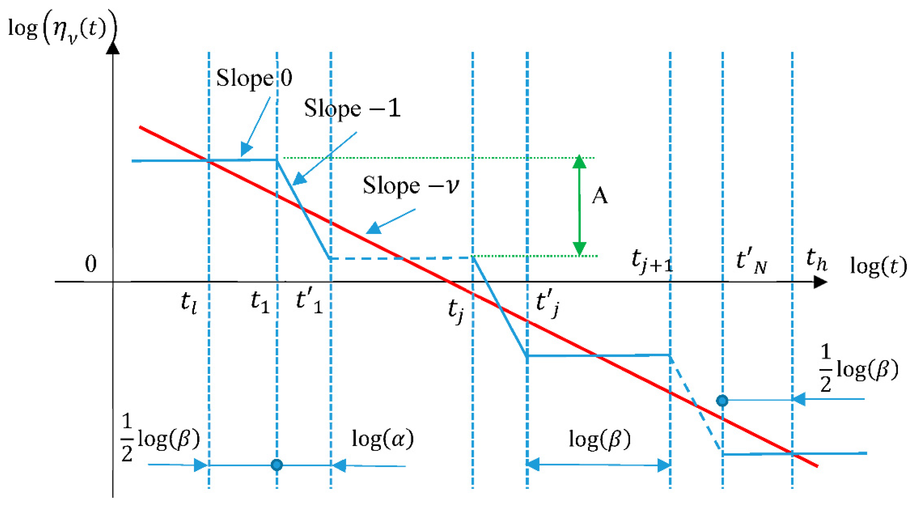
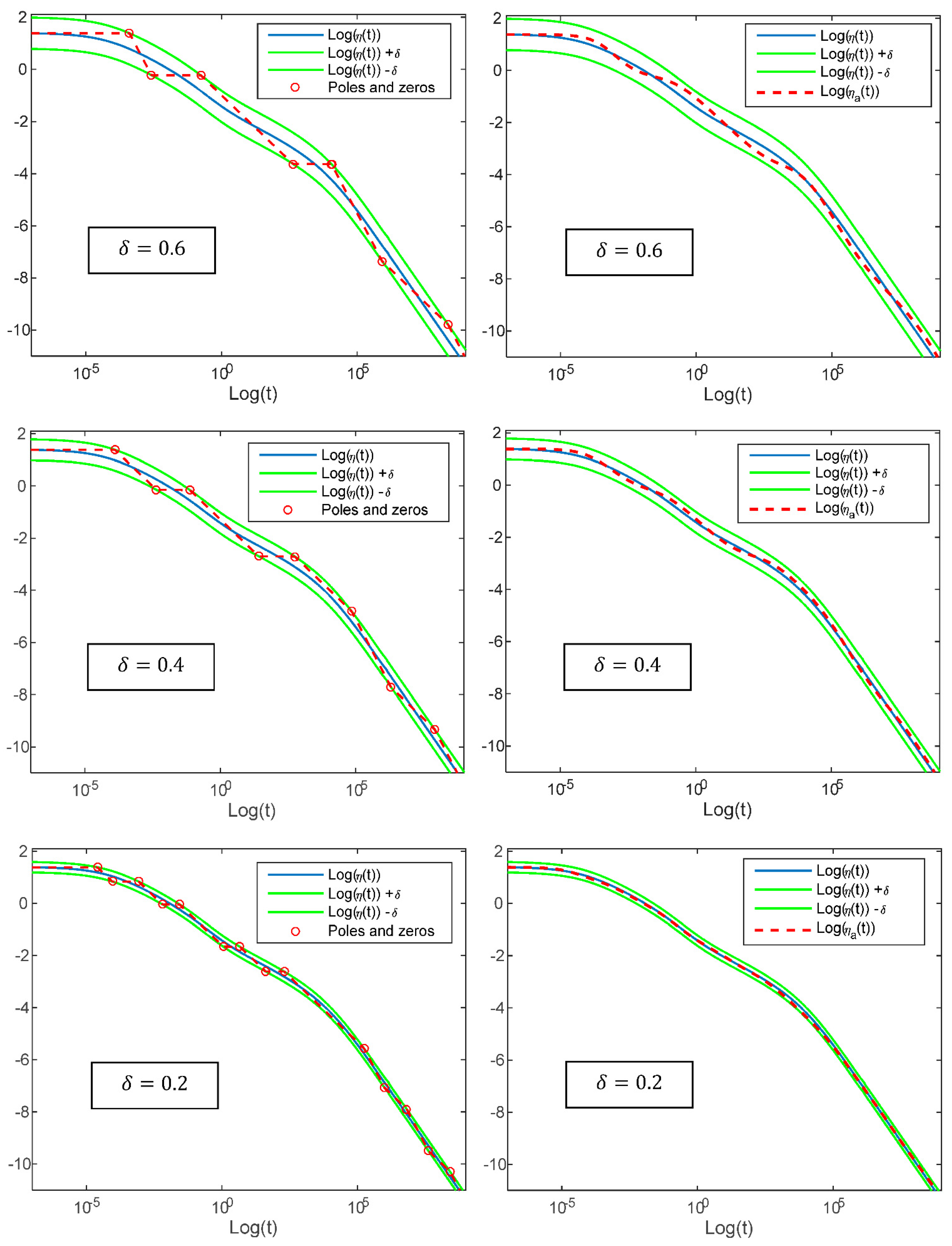
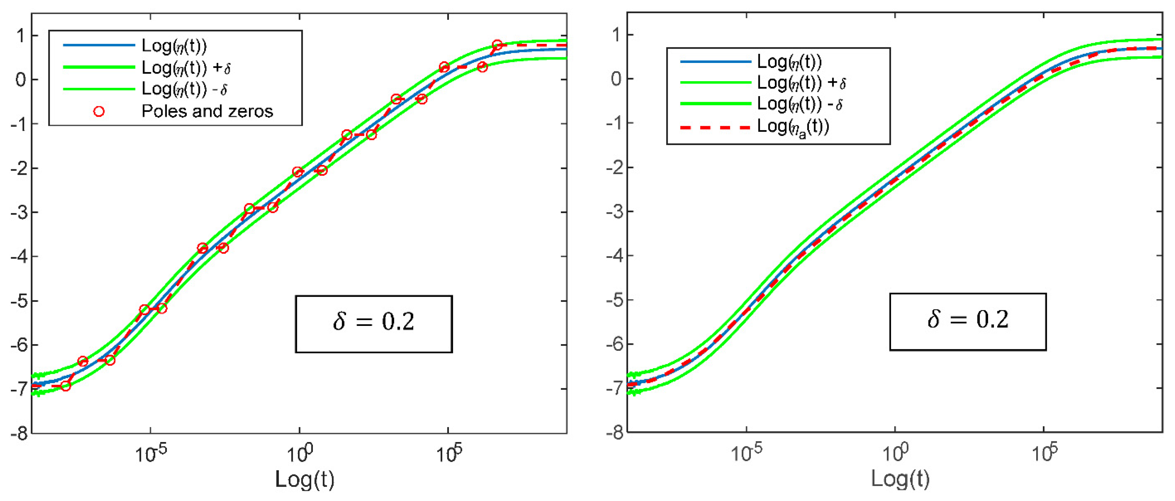
on the left, how poles and zeros are added in ${\eta }_a\left(t\right)$ as the asymptotic behavior of this function intersects the upper and lower bounds.

-

on the right, the resulting function ${\eta }_a\left(t\right)$.

This figure demonstrates the efficiency of the proposed algorithm to fit a fractional behavior. It also shows that it is possible to control the accuracy of this fitting through parameter $\delta$. This is confirmed by the calculation of the absolute error

$${\epsilon }_a=\frac{1}{N_s}{\sum }_{k=1}^{N_s}{\left({\eta }_a\left(k\right)-\eta \left(k\right)\right)}^2 N_s=\mathrm{10,000}$$

(36)

for the three values of $\delta$ considered. These errors ${\epsilon }_a$, reported in Table 1, decrease as $\delta$ decreases.

Table 1. Comparison of $\eta \left(t\right)$ and ${\eta }_f\left(t\right)$.

$\mathit{\delta }$	0.2	0.4	0.6
${\epsilon }_a$	2.077 × 10−1	2.0472	3.9617

This comparison permits us to say that, even if I + f convergence of the kernel is slow as the time tends towards infinity, the fitting method described by Algorithm 2 remains possible. The order of the fraction will increase, but it is still possible. Nevertheless, it must be mentioned that, when working in the logarithmic domain, a sort of time compression occurs which facilitates fitting over large time domains.

Another kind of impulse response is now considered, the one produced by the transfer function (30) and which is defined analytically by relation (31). The result obtained with Algorithm 2 is shown in Figure 8 and reveals again times the impulse response fitting in compliance with the imposed bound.

Figure 8. Comparison of $\eta \left(t\right)$ and ${\eta }_a\left(t\right)$ for the impulse response of model (27) with $\delta =0.2$. left column: asymptotic diagram built by the algorithm, right column: obtained function ${\eta }_a\left(t\right)$.

4. Conclusions

In this paper, several algorithms are proposed to fit a fractional dynamical behavior using a convolution integral involving a rational kernel. In the case of a pure power law function, a first algorithm based on an interlacing distribution of poles and zeros in the rational kernel is given. Using a logarithmic scale on the abscissa and ordinate axes, a power law function of order $\nu$ ($K{t}^{-\nu })$ appears as a line of slope $-\nu$. It is thus possible to approximate it by interlacing poles and zeros which, respectively, induce in this same system of coordinates, an asymptotic behavior of slope −1 and 1. It is then demonstrated that the values of the poles and zeros are linked by geometric ratios that are computed by the algorithm. This fitting solution appears to be similar to the one commonly used in the frequency domain to approximate the behavior of a fractional integrator or differentiator. In fact, it is observed that the solution proposed here in the time domain leads to fewer oscillations for the same number of poles and zeros.

Inspired by the idea of interlacing of poles and zeros, a second algorithm is proposed to fit the impulse response of a system with any fractional dynamical behavior. First, we propose a solution based on a least squares method to derive the sampled-data impulse response of a dynamical system from input-output data. Then, the solution to obtain an approximant of this impulse response in the form of a rational function consists of adding poles or zeros in the approximant so that the error remains bounded in absolute value. This algorithm adds a pole if the approximant asymptotic diagram induced by the pole or the zeros previously added intersects the selected upper bound, and vice versa, a zero is added if the asymptotic diagram of the approximant induced by the pole or the zero previously added intersects the lower bound. In the applications proposed in the paper that illustrate the algorithm’s efficiency, a constant error bound is imposed over the whole approximation time interval. However, this algorithm also works by taking different upper and lower bounds and functions of time. This algorithm is able to place the poles and zeros of the approximation and limit the approximation error between an upper and lower bound, but this placement is sub-optimal with regard to the quadratic error between the impulse response and its approximation. Moreover, this sequence of two algorithms (kernel samples computation using the algorithm described in Section 3.1 and then fitting the kernel samples with a rational kernel using Algorithm 2) can lead to the accumulation of errors. Furthermore, although Algorithm 2, which is recursive, has a low chance of leading to numerical instabilities, the algorithm used in Section 3.1 may have some. On the other hand, the solution we propose is very simple to implement and can constitute a solution for initializing future algorithms which will be developed by the authors. The authors have also now to consider additional real-life fractional behavior in order to clearly identify the limits of the use of non-singular rational kernels in modeling situations and to consider possible significant changes over time in the modelled system behavior.

This work is an additional illustration that fractional behaviors can be modelled using other tools than the ones based on fractional calculus.

References

- Caputo, M.; Fabrizio, M. A new definition of fractional derivative without singular kernel. Prog. Fract. Differ. Appl. 2015, 1, 73–85. [Google Scholar]
- Atangana, A.; Baleanu, D. New fractional derivatives with nonlocal and non-singular kernel: Theory and application to heat transfer model. Therm. Sci. 2016, 20, 763–769. [Google Scholar] [CrossRef]
- Hristov, J. Derivatives with Non-Singular Kernels from the Caputo-Fabrizio Definition and Beyond: Appraising Analysis with Emphasis on Diffusion Models. In Frontiers in Fractional Calculus; Chapter 10; Bentham Science Publishers: Sharjah, United Arab Emirates, 2017. [Google Scholar]
- Saad, K.M.; Atangana, A.; Baleanu, D. New fractional derivatives with non-singular kernel applied to the Burgers equation. Chaos 2018, 28, 063109. [Google Scholar] [CrossRef] [PubMed]
- Hattaf, K. A New Generalized Definition of Fractional Derivative with Non-Singular Kernel. Computation 2020, 8, 49. [Google Scholar] [CrossRef]
- Sabatier, J.; Farges, C.; Tartaglione, V. Fractional Behaviours Modelling: Analysis and Application of Several Unusual Tools, Intelligent Systems, Control and Automation: Science and Engineering Series; Springer: Cham, Switzerland, 2022; Volume 101. [Google Scholar]
- Sabatier, J. Modelling Fractional Behaviours without Fractional Models. Front. Control. Eng. 2021, 2, 716110. [Google Scholar] [CrossRef]
- Dokoumetzidis, A.; Magin, R.; Macheras, P. A commentary on fractionalization of multi-compartmental models. J. Pharmacokinet. Pharmacodyn. 2010, 37, 203–207. [Google Scholar] [CrossRef] [PubMed]
- Sabatier, J.; Farges, C.; Trigeassou, J.-C. Fractional systems state space description: Some wrong ideas and proposed solutions. J. Vib. Control 2014, 20, 1076–1084. [Google Scholar] [CrossRef]
- Balint, A.M.; Balint, S. Mathematical Description of the Groundwater Flow and that of the Impurity Spread, which Use Temporal Caputo or Riemann–Liouville Fractional Partial Derivatives, Is Non-Objective. Fractal Fract. 2020, 4, 36. [Google Scholar] [CrossRef]
- Sabatier, J.; Farges, C.; Tartaglione, V. Some Alternative Solutions to Fractional Models for Modelling Power Law Type Long Memory Behaviours. Mathematics 2020, 8, 196. [Google Scholar] [CrossRef]
- Sun, H.; Wang, Y.; Yu, L.; Yu, X. A discussion on nonlocality: From fractional derivative model to peridynamic model. Commun. Nonlinear Sci. Numer. Simul. 2022, 114, 106604. [Google Scholar] [CrossRef]
- Pantokratoras, A. Comment on the paper “Fractional order model of thermo-solutal and magnetic nanoparticles transport for drug delivery applications, Subrata Maiti, Sachin Shaw, G.C. Shit”. Colloids Surf. B Biointerfaces 2023, 222, 113074. [Google Scholar] [CrossRef] [PubMed]
- Pantokratoras, A. Discussion on the paper “A Numerical Scheme for Fractional Mixed Convection Flow Over Flat and Oscillatory Plates, Yasir Nawaz, Muhammad Shoaib Arif, Kamaleldin Abodayeh”. J. Comput. Nonlinear Dyn. 2022, 17, 071008. [Google Scholar]
- Podlubny, I. Fractional Differential Equations. In Theoretical Developments and Applications in Physics and Engineering Mathematics in Sciences and Engineering; Academic Press: Cambridge, MA, USA, 1999. [Google Scholar]
- Samko, S.G.; Kilbas, A.A.; Marichev, O.I. Fractional Integrals and Derivatives: Theory and Applications; Gordon and Breach Science Publishers: London, UK, 1993. [Google Scholar]
- Sabatier, J. Fractional Order Models Are Doubly Infinite Dimensional Models and thus of Infinite Memory: Consequences on Initialization and Some Solutions. Symmetry 2021, 13, 1099. [Google Scholar] [CrossRef]
- Ortigueira, M.D.; Coito, F.J. System initial conditions vs derivative initial conditions. Comput. Math. Appl. 2010, 59, 1782–1789. [Google Scholar] [CrossRef]
- Sabatier, J.; Farges, C. Comments on the description and initialization of fractional partial differential equations using Riemann–Liouville’s and Caputo’s definitions. J. Comput. Appl. Math. 2018, 339, 30–39. [Google Scholar] [CrossRef]
- Sabatier, J.; Farges, C.; Merveillaut, M.; Fenetau, L. On observability and pseudo state estimation of fractional order systems. Eur. J. Control 2012, 18, 260–271. [Google Scholar] [CrossRef]
- Newman, D.J. Newman, Rational approximation to |x|. Mich. Math. J. 1964, 11, 11–14. [Google Scholar] [CrossRef]
- Lether, F.G. Thiele Rational Interpolation for the Numerical Computation of the Reversible Randles–Sevcik Function in Electrochemistry. J. Sci. Comput. 1999, 14, 259–274. [Google Scholar] [CrossRef]
- Nakatsukasa, Y.; Sète, O.; Trefethen, L.N. The AAA Algorithm for Rational Approximation. SIAM J. Sci. Comput. 2018, 40, A1494–A1522. [Google Scholar] [CrossRef]
- Filip, S.-I.; Nakatsukasa, Y.; Trefethen, L.N.; Beckermann, B. Rational Minimax Approximation via Adaptive Barycentric Representations. SIAM J. Sci. Comput. 2018, 40, A2427–A2455. [Google Scholar] [CrossRef]
- DeVore, R.A. Approximation by Rational Functions. Proc. Am. Math. Soc. 1986, 98, 601–604. [Google Scholar] [CrossRef][Green Version]
- Cuyt, A. Rational Approximation Theory: A state of the art. Acta Appl. Math. 1993, 33, 119. [Google Scholar] [CrossRef]
- Manabe, S. The non-integer Integral and its Application to control systems. ETJ Jpn. 1961, 6, 83–87. [Google Scholar]
- Carlson, G.E.; Halijak, C.A. Simulation of the Fractional Derivative Operator and the Fractional Integral Operator. Available online: http://krex.k-state.edu/dspace/handle/2097/16007 (accessed on 15 January 2008).
- Ichise, M.; Nagayanagi, Y.; Kojima, T. An analog simulation of non-integer order transfer functions for analysis of electrode processes. J. Electroanal. Chem. Interfacial Electrochem. 1971, 33, 253–265. [Google Scholar] [CrossRef]
- Oustaloup, A. Systèmes Asservis Linéaires d’ordre Fractionnaire; Masson: Paris, France, 1983. [Google Scholar]
- Raynaud, H.-F.; Zergaïnoh, A. State-space representation for fractional order controllers. Automatica 2000, 36, 1017–1021. [Google Scholar] [CrossRef]
- Charef, A. Analogue realisation of fractional-order integrator, differentiator and fractional PIλDµ controller. IEE Proc. Control Theory Appl. 2006, 153, 714–720. [Google Scholar] [CrossRef]
Disclaimer/Publisher’s Note: The statements, opinions and data contained in all publications are solely those of the individual author(s) and contributor(s) and not of MDPI and/or the editor(s). MDPI and/or the editor(s) disclaim responsibility for any injury to people or property resulting from any ideas, methods, instructions or products referred to in the content. |
© 2023 by the authors. Licensee MDPI, Basel, Switzerland. This article is an open access article distributed under the terms and conditions of the Creative Commons Attribution (CC BY) license (https://creativecommons.org/licenses/by/4.0/).