Leveraging Machine Learning for Weed Management and Crop Enhancement: Vineyard Flora Classification

Abstract

The global population’s rapid growth necessitates a 70% increase in agricultural production, posing challenges exacerbated by weed infestation and herbicide drawbacks. To address this, machine learning (ML) models, particularly convolutional neural networks (CNNs), are employed in precision agriculture (PA) for weed detection. This study focuses on testing CNN architectures for image classification tasks using the PyTorch framework, emphasizing hyperparameter optimization. Four groups of experiments were carried out: the first one trained all the PyTorch architectures, followed by the creation of a baseline, the evaluation of a new and extended dataset in the best models, and finally, the test phase was conducted using a web application developed for this purpose. Of 80 CNN sub-architectures tested, the MaxVit, ShuffleNet, and EfficientNet models stand out, achieving a maximum accuracy of 96.0%, 99.3%, and 99.3%, respectively, for the first test phase of PyTorch classification architectures. In addition, EfficientNet_B1 and EfficientNet_B5 stood out compared to all other models. During experiment 3, with a new dataset, both models achieved a high accuracy of 95.13% and 94.83%, respectively. Furthermore, in experiment 4, both EfficientNet_B1 and EfficientNet_B5 achieved a maximum accuracy of 96.15%, the highest one. ML models can help to automate crop problem detection, promote organic farming, optimize resource use, aid precision farming, reduce waste, boost efficiency, and contribute to a greener, sustainable agricultural future.

1. Introduction

By 2050, the world’s population is expected to grow significantly to nine billion people. To satisfy the expected demands, agricultural production must rise by almost 70%. The agricultural industry will nevertheless face several difficulties at that time, including a decline in the amount of arable land and the requirement for more intense production. Productivity will also be impacted by additional problems, such as climate change and water shortages [1].

The productivity and quality of crops can be affected by prejudicial vegetation because of its ability to spread fast and unintentionally. In the battle for food, water, sunlight, and growth space, unwanted plants face up to crops. Numerous factors affect how control tactics are employed to lessen their impact [1].

An over-dependence on herbicides can harm the environment, cause non-target crop damage, destroy natural flora and soil biodiversity, and be harmful to the general public’s and farmworkers’ health [2]. Herbicide administration may be decreased by 40% on average by employing extensive information on the types of weed plants that have emerged, their growth phases, and plant densities in a field [3].

Due to rising labor expenses and an increase in public concern for their health and the environment, automation in weed management has gained popularity. Automated vegetation control methods may be useful from a sustainability and financial perspective [1]. With its continued development, artificial intelligence (AI) is finding more and more benefits in agriculture. The Internet of Things (IoT) and the 4th Industrial Revolution (Industry 4.0) both provide new opportunities for innovation [4].

Image classification, a subfield of computer vision, plays a crucial role in modernizing the agricultural industry. By utilizing advanced machine learning techniques, such as deep learning (DL) and AI, image recognition has the potential to transform traditional farming practices and enhance productivity [4]. Thus, the detection and classification of flora has been a focus of several machine learning (ML)-based algorithms’ development, making it a potential topic of research [5]. DL techniques provide several benefits for picture classification, object identification, and recognition [1].

In recent years, convolutional neural networks (CNNs) have emerged as a game-changing technology, revolutionizing the field of image classification. With their unique architecture and sophisticated algorithms, CNN models have propelled the accuracy and efficiency of image analysis to unprecedented levels [2]. A strong framework for creating, developing, and deploying neural network (NN) models is offered by PyTorch [1,6].

As we move forward into an increasingly visual world, the importance of CNN models for accurate image classification and understanding cannot be overstated, opening new possibilities and driving innovation across a wide range of domains. In this paper, a study about the different types of NN models for image classification available in PyTorch was conducted. The objective of this work was to study and understand how different models work as well as which one was the best, according to the experiments carried out. The proposal aims to discover which model is the best with both a small and large dataset.

This paper is organized into four sections. Section 1 includes an introduction to the agricultural problem as well as a shortage of the suggested solution. Section 2 presents the literature related to the task of weed classification. Section 3 presents the materials and methods used in the suggested solution. Section 4 presents all the experiments and results achieved. Section 5 presents a discussion of the results, considering the groups of experiments carried out in Section 4. Finally, Section 6 presents the conclusions of this work.

2. Related Work

2.1. Neural Network Architectures

CNN models improve image analysis accuracy and efficiency. PyTorch, an open-source platform, offers flexibility, intuitiveness, and dynamic computing graphs for building and training NNs. With twenty different architectures, and multiple sub-architectures, it offers distinct models for various image classification tasks [7].

AlexNet and Visual Geometry Group (VGG) are both influential convolutional neural network architectures for image classification. AlexNet was one of the first deep models to gain widespread attention, employing five convolutional layers with max pooling and three fully connected layers. VGG is characterized by its simplicity, consisting of deeper convolutional layers (up to 19 layers) with small 3 × 3 kernels and max pooling, followed by fully connected layers. While AlexNet emphasizes the use of Rectified Linear Unit (ReLU) activations and dropout for regularization, VGG focuses on exploring the impact of increasing network depth, paving the way for subsequent deep architectures [8]. ConvNeXt employs group convolutions and path aggregation to efficiently learn features by dividing input channels into groups. It balances computational efficiency and representational strength using cardinality, offering various depth and capacity options [9]. SqueezeNet focuses on compactness, utilizing 1 × 1 convolutions and skip connections to reduce parameters and address gradient flow issues. It strikes a balance between model size and accuracy, making it ideal for devices with limited resources [10]. RegNet adopts compound scaling and adaptive rules, allowing uniform adjustment of network depth, width, and resolution, providing flexibility in customizing model capacity and computational resources [11].

GoogLeNet introduced inception modules employing parallel convolutional processes with filter sizes of 1 × 1, 3 × 3, and 5 × 5, along with max pooling, effectively capturing local and global information. Also, 1 × 1 convolutional layers are used for dimensionality reduction, optimizing computational resources. Auxiliary classifiers, with fully connected and 1 × 1 convolutional layers, address the vanishing gradient problem, promoting distinctive feature learning. GoogLeNet employs global average pooling instead of fully connected layers, minimizing overfitting. With 22 layers and more filters per layer, it showcases advanced performance in deep learning applications [9]. InceptionV3 is an evolution of GoogLeNet. It is a newer version with deeper architecture and fewer parameters, making it more efficient and accurate. It uses innovative inception modules and factorized convolutions, allowing it to capture features at various scales [12].

DenseNet and Residual Network (ResNet) are both deep neural network architectures. DenseNet achieves dense connectivity by connecting each layer to every other layer in a feed-forward structure. This promotes feature reuse and addresses the vanishing gradient problem. It emphasizes dense connections between layers, where each layer receives direct input from all preceding layers, promoting feature reuse and gradient flow. DenseNet’s dense connections lead to parameter efficiency and feature reuse, enabling better gradient flow [10]. ResNet also utilizes a similar concept of residual connections, ensuring smooth gradient flow during training, allowing for the easy training of very deep networks by learning residual functions. ResNet’s residual connections help in mitigating vanishing gradient problems, enabling the training of very deep networks. Both approaches have significantly impacted deep learning but employ different strategies for information propagation within the network [13].

ResNeXT and Wide ResNet are variants of the original ResNet architecture. ResNet introduces residual blocks. ResNeXt enhances ResNet by using a split–transform–merge strategy, aggregating information through parallel paths, and improving representational capacity [14]. Wide ResNet, on the other hand, increases the width of residual blocks, leading to a wider network with more feature channels, enhancing the capacity for capturing complex patterns [15]. While ResNet focuses on depth, ResNeXT emphasizes multi-path aggregation and Wide ResNet emphasizes increased width, providing different strategies for improving the expressiveness and learning capabilities of deep neural networks [14,15].

ViT (Vision Transformer), Swin Transformer, and MaxVit are advanced DL architectures for computer vision tasks. ViT pioneered the transformer architecture for vision tasks, using self-attention mechanisms to process image patches directly, but it struggles with handling large images due to quadratic complexity. It integrates self-attention layers and feed-forward networks to process patch embeddings [16]. The Swin Transformer introduces hierarchical transformers, organizing layers into stages and allowing cross-stage information flow, enabling efficient parallel processing of image patches [17]. MaxVit addresses ViT’s limitations by introducing a novel variant with a maximal pooling strategy, reducing computational complexity while maintaining strong performance on large images. Each approach provides unique solutions to leverage transformers for image understanding, catering to different computational and task-specific requirements. The architecture uses multi-axis attention and convolution, processing input images with a convolutional stem. It employs mobile inverted bottleneck convolution blocks for computational efficiency and a grid structure for object recognition and pattern analysis [18].

Both MobileNet and ShuffleNet V2 architectures focus on computational efficiency for mobile and edge devices and aim to reduce computational cost and model size while maintaining accuracy. MobileNet uses depth-wise separable convolutions and introduces width and depth multipliers, allowing adjustments between model size and accuracy [10]. ShuffleNet V2 combines depth-wise convolutions with compact 1 × 1 convolutions and introduces channel shuffling and pointwise group convolutions, enabling efficient information exchange across channels and reducing computational complexity further [19]. This process starts with the “Channel Split” procedure, where the input feature map’s channels are divided into two branches of equal size. One branch remains unaltered, while the other undergoes three convolution layers. The outputs of these branches are then merged using the concatenation operation, “Concat”, after convolution, ensuring an equal number of channels in the combined output. Subsequently, the “channel shuffle” mechanism is applied, enabling effective communication and interaction between these branches [10,19].

EfficientNet, EfficientNetV2, and MNASNet are designed with a focus on efficient scaling. EfficientNet optimizes model size, depth, and width simultaneously using compound scaling, providing a balanced trade-off between accuracy and computational cost [20]. EfficientNetV2, an evolution of it, refines the design principles, introducing improved factorized convolutions for enhanced efficiency and accuracy [11]. MNASNet employs an automated neural architecture search (NAS) to discover efficient model architectures and customize networks to specific hardware constraints and use cases [20]. While EfficientNet and EfficientNetV2 focus on efficient scaling, MNASNet emphasizes automated search methods, offering distinct approaches to achieving efficiency and accuracy in neural network design.

2.2. Experimental Studies—Flora Classification

Traditional methods of flora identification require considerable time and expertise. DL techniques can expedite this process by analyzing real-world data and providing faster and more accurate results [21].

Also, irrigation planning is crucial in agriculture for maintaining constant yield and reducing water shortage risks, as it accounts for a significant portion of total water use.

Some studies, like Alibabaei et al. [22] propose the development of an automatic irrigation system using advanced technologies, specifically leveraging deep learning algorithms. This study employs a Deep Q-Network (DQN) for optimizing irrigation scheduling in a tomato field in Portugal. The DQN agent interacts with two Long Short Term Memory (LSTM) models, serving as the environment. One LSTM model predicts the next day’s total water content in the soil, while the other estimates crop yield based on seasonal environmental conditions, calculating the net return. The agent uses this information to determine the necessary irrigation amount.

During training, three neural network architectures—Artificial Neural Network (ANN), LSTM, and Convolutional Neural Network (CNN)—are utilized to estimate the Q-table, a critical component in reinforcement learning. Notably, the study observes that, unlike the LSTM model, both the ANN and CNN struggle to accurately estimate the Q-table, resulting in a reduction in the agent’s reward during training. The trained DQN model exhibits promising results, enhancing productivity by 11% and reducing water consumption by 20–30% compared to a traditional method.

Dyrmann et al. [3] developed a CNN for plant species identification in colored photos, utilizing six datasets containing images from controlled and natural environments with varying lighting. The training set underwent augmentation and preprocessing, including excessive green segmentation. The overall accuracy of the model averaged 86.2%. Classes with more species generally exhibited better accuracy, highlighting challenges faced by classes with limited photo samples.

Andrea et al. [23] developed an algorithm for the real-time segmentation and classification of plants using CNNs. Four CNN models (LeNet, AlexNet, cNet, and sNet) were employed to differentiate maize plants from weeds using RGB (red, green, blue) and Near-Infrared (NIR) images obtained from a multispectral camera. The images were processed to enhance green color detection and then converted to grayscale to distinguish plants from non-plant features. The cNet model with 16 filters showed the best performance, achieving a training accuracy of 97.23%.

Gao et al. [24] proposed using a hyperspectral NIR snapshot camera to classify weeds and maize. They identified critical spectral wavelengths and characteristics for classification using the Normalized Difference Vegetation Index (NDVI) and Radar Vegetation Index (RVI). ML techniques, including feature engineering and image processing, were applied to construct a Random Forest (RF) model. The RF model achieved high recalls, 100% for maize, 78.9% for Convolvulus arvensis, 69.1% for Rumex, and 75.2% for Cirsium arvense, and high accuracies and F1 scores for differentiating crops and weeds.

Bakhshipour and Jafari [25] developed a classification system for sugar beet crops and four weed types using shape features and image segmentation techniques. They used support vector machine (SVM) and artificial neural network (ANN) classifiers. For sugar beet classification, SVM achieved 96.67% accuracy and ANN achieved 93.33%. For weed classification, SVM and ANN both attained 92.50% accuracy. The shape-based weed detection algorithm successfully distinguished sugar beets and weeds, using red pixels for weeds, green pixels for sugar beets, and yellow pixels for misclassified areas. They also presented a visual representation of their model’s outcomes. NIR, red, and NDVI images were used as input data for the CNN, with the model’s probability output displaying crops in red, weeds in green, and the background in blue, compared against annotated ground truth.

Sa et al. [26] employed multispectral data captured by a Micro Aerial Vehicle (MAV) to classify sugar beetroot and weed species using CNN. They converted the data into SegNet format, categorizing images into crops, weeds, or both, using NDVI and image processing to differentiate vegetation. Six models with varying input channel sizes were trained and evaluated using F1 scores and AUC measures. The best model achieved an 80% average F1 score and accuracy on test data, showing promise in classifying crops and weeds despite dataset limitations.

In a separate study, Yang et al. [27] explored DL methods for hyperspectral image classification. They developed and refined four models: two-dimensional CNN (2-D-CNN), three-dimensional CNN (3-D-CNN), 2D CNN based on regions (R-2-D-CNN), and 3D CNN with a regional focus (R-3-D-CNN). These models considered both spectral and spatial factors. The R-2-D-CNN and R-3-D-CNN models achieved exceptional accuracy rates, with the R-3-D-CNN reaching 99.87% and 99.97% accuracy in one dataset, emphasizing the importance of spectral and spatial considerations in hyperspectral image classification.

In a related study developed by [28], a DL technique using KERAS API and TensorFlow backend was employed for the picture classification of nine different crops and their corresponding weeds. The model achieved an impressive accuracy rate of 96.3% by correctly categorizing plants and weeds using 250 images of each plant type acquired in the field. The model’s accuracy highlighted its effectiveness in distinguishing between crops and weeds for agricultural applications.

Jin et al. [29] developed a sophisticated algorithm to identify weeds in vegetable plantations. The algorithm utilized CenterNet, representing objects as single points with object centers predicted using a heatmap. Ground truth key points were transformed into smaller key-point heatmaps through a Gaussian kernel and focal loss for network training. Weeds were identified as green objects outside the annotated bounding boxes.

The trained CenterNet model exhibited a very good performance with a precision of 95.6%, recall of 95.0%, and F1 score of 95.3%. It successfully identified vegetables under various conditions, presenting the final segmentation results with vegetable regions highlighted in red boxes.

El-Kenawy et al. [30] introduced a novel approach for classifying weeds in wheat photos taken by a drone. Three machine learning models, ANN, SVM, and the K-nearest neighbors’ algorithm (KNN), were utilized. AlexNet was used with a binary optimizer to enhance feature selection. This approach achieved a detection accuracy of 97.70%, F1 score of 98.60%, specificity of 95.20%, and sensitivity of 98.40%, outperforming other methods.

Koparan et al. [31] investigated weed detection using DL models (VGG16 and ResNet50) with varying backgrounds. Images of weeds and crops were captured with different backgrounds (uniform and non-uniform). The models showed better performance on images like their training backgrounds. A model trained with combined datasets achieved an F1 score between 92% and 99%.

Zhang et al. [32] compared SVM and VGG16 DL classifiers using RGB images to classify weeds and crop species. Image processing techniques were employed to extract the green portion of the pictures, followed by feature extraction using Local Binary Pattern (LBP) and Gray-level Co-occurrence Matrix (GLCM) features. The VGG16 model outperformed SVM, with F1 score results ranging from 93% to 97.5%.

Thus, advances in image processing, spectral analysis, and model development have contributed to more accurate and efficient methods for classifying plants and weeds. These studies demonstrate the effectiveness of DL and ML techniques in flora classification, offering promising results for various applications in agriculture and plant species identification. However, hardware costs for high-end cameras (multispectral and hyperspectral), data limitations, potential overfitting, computational resource requirements, model complexity, and challenges associated with real-world deployment and interpretability limit the field applicability of these models. Thus, this paper aims to contribute to this topic by testing CNN architectures using the PyTorch framework, emphasizing hyperparameter optimization. It aims to assess the best models to be integrated into technological systems and methods for selective weed removal such as automatic herbicide sprayers, mechanical removal, thermal weeders, high-intensity laser weeders, and electric weeding devices, among others.

3. Materials and Methods

This chapter explores the scientific knowledge development through careful material and method selection, focusing on the PyTorch framework, and data analysis, providing insights into algorithm evolution and simulation. The experiments were conducted on a computer with an NVIDIA GeForce RTX 2080 SUPER, Intel i7-4790 (8-core) CPU, and 32 GB RAM.

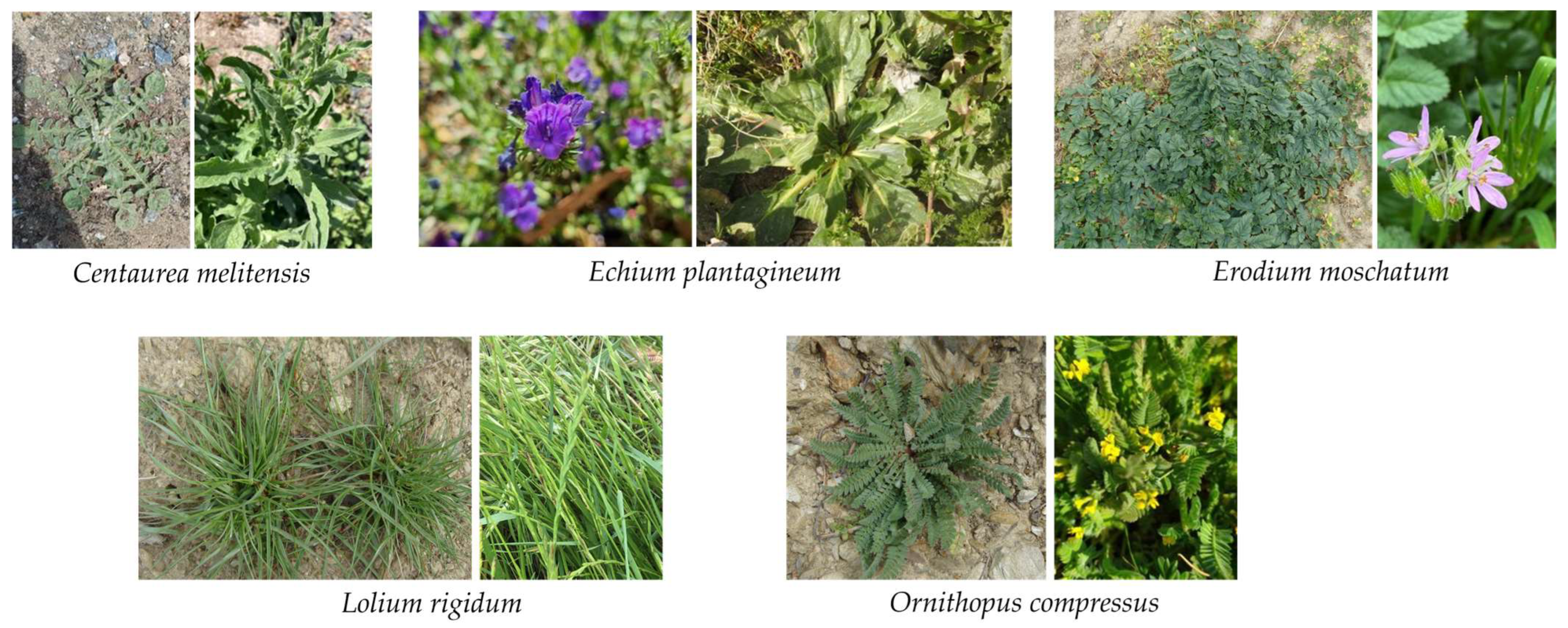
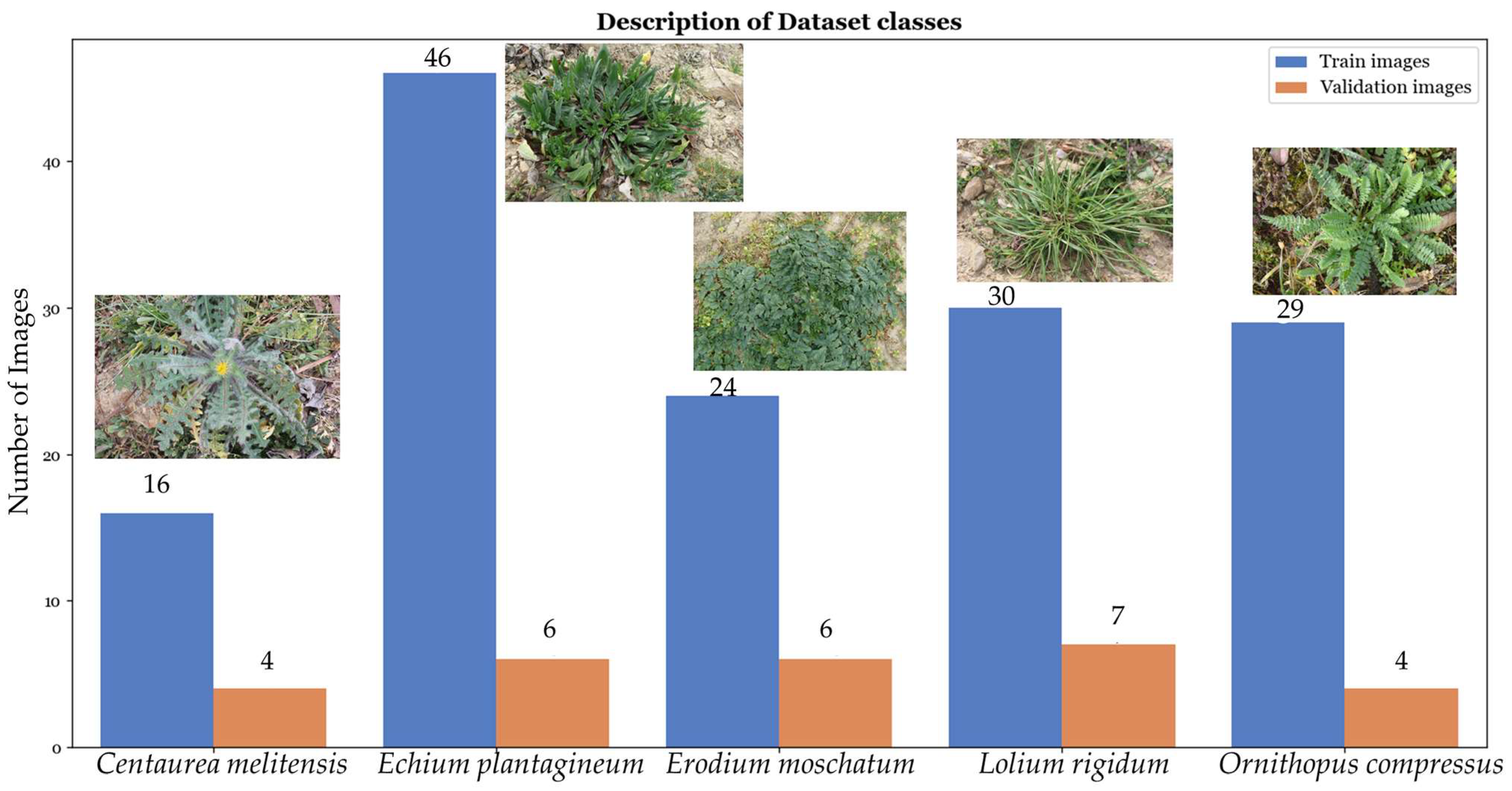
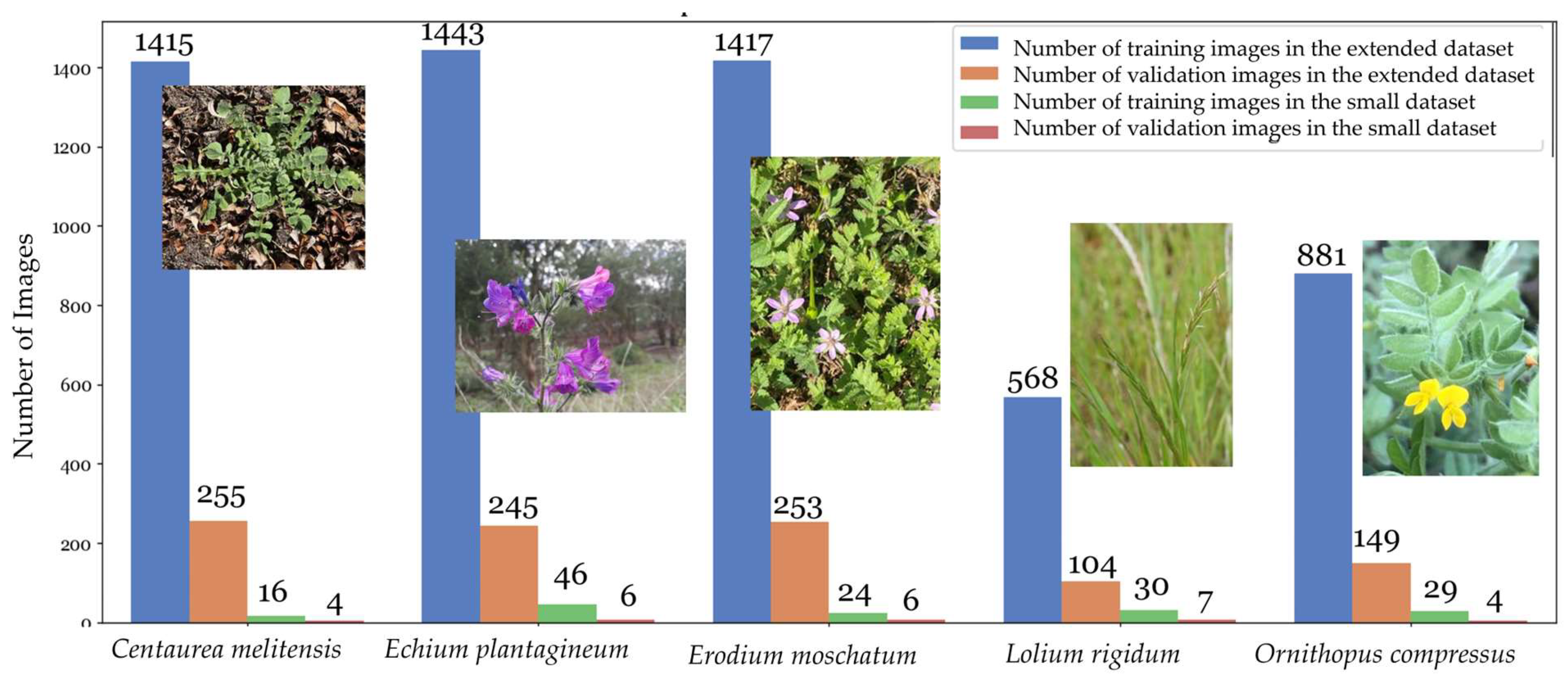
3.1. Data Collection and Sample Preparation

In this study, a dataset comprising 172 images of vineyard flora was collected using a Sony RGB Camera DSC-RX100M2 (sensor: type 1.0 (13.2 × 8.8 mm) Exmor R^® CMOS sensor; number of pixels approx. 20.2 Megapixels; lens: ZEISS^® Vario-Sonnar^® T* Lens; optical zoom 3.6×; angle of view (35 mm format equivalent) 75°–24° (28–100 mm); focal length (F=) f = 10.4–37.1 mm). The images were taken during the spring and autumn seasons in the Douro Natural Park. The images covered five weed classes: Centaurea melitensis, Echium plantagineum, Erodium moschatum, Lolium rigidum, and Ornithopus compressus. Figure 1 shows examples of the species used to test the architectures available for the classification task in the PyTorch framework.

Figure 1. Representation of the five species in the image classification task.

The initial dataset was divided into training (85% of images, 145 images) and validation (15% of images, 27 images) sets following established protocols [33].

The distribution of images for each species in both the training (represented in blue) and validation (represented in orange) sets is shown in Figure 2.

Figure 2. The initial dataset, comprising 172 images, underwent a precise division for training and validation, emphasizing the visualization of species-specific data distribution. The division is graphically represented with a blue line indicating the number of images allocated for the training set and an orange line depicting the number of images designated for validation for each species.

3.2. Algorithm Execution

The study focuses on finding the most effective model for classifying vineyard flora through experiments involving various hyperparameter combinations. Hyperparameters such as batch size, number of epochs, learning rate, weight decay, and number of fully connected layers significantly influence the model’s learning and performance.

The batch size, limited to four due to memory constraints, represents the number of samples processed before updating the model. The number of epochs determines how many times the learning algorithm processes the training dataset [34].

The learning rate present in optimization algorithms controls the step size during the iterative process of updating model parameters to minimize the loss function. Weight decay is a regularization technique in machine learning that discourages overly complex models by adding a penalty term to the loss function, effectively reducing the magnitudes of the model parameters [35].

The number of fully connected layers in a neural network refers to the depth of the network architecture, which determines the network’s capacity for modeling complex functions, with two tested configurations: linear (Lin.) and sequential (Seq.) [36].

In neural network terminology, fully connected layers are integral components of a neural network architecture. In these layers, every neuron is linked to all neurons in both the preceding and subsequent layers. This intricate interconnection allows each neuron to receive input from every neuron in the previous layer and transmit its output to all neurons in the subsequent layer. When referring to a linear number of layers, the number of neurons in the last layer was replaced with the number of classes. On the other hand, in a sequential number of layers, layers were modified and added to decrease the original number of neurons until the number of classes was reached [1].

Twelve different hyperparameter combinations were explored for each model, aiming to identify optimal settings for vineyard flora classification. These combinations were carefully chosen and tested for each architecture. Different combinations of hyperparameters refer to various configurations of the adjustable parameter values in an ML algorithm. Exploring different combinations allowed us to find the ideal configuration to optimize the model’s performance. Thus, the learning rate used three different values (0.01, 0.001, and 0.0001), the weight decay used two values (0 and 0.0001), and the two configurations of layers (Lin. and Seq.). According to these values, all the hyperparameters were joined to create the 12 combinations.

Furthermore, the inference time of the models was tested as well. The inference time for each image was measured independently, and the average inference time across all photos was calculated. The inference time was used to determine whether there are substantial variances in execution time. The distribution of these times can reveal how consistently the model works across diverse inputs. The average inference time provides a broad assessment of the model’s efficiency throughout the whole test set. If the average time is reasonable and consistent, it indicates stable performance.

The metric used to evaluate the models was accuracy (acc). This is a metric used to measure the proportion of correct predictions made by a model, expressed as the ratio of accurate predictions to the total predictions. The calculation of the accuracy is represented in Equation (1), where True Positive (TP) represents the correctly predicted positive-class samples, while True Negative (TN) indicates the accurately predicted negative-class samples. False Positive (FP) refers to negative-class samples incorrectly predicted as positive, and False Negative (FN) signifies positive-class samples inaccurately predicted as negative [1].

$$\mathrm{a}\mathrm{c}\mathrm{c}=\frac{\mathrm{T}\mathrm{P}+\mathrm{T}\mathrm{N}}{\mathrm{T}\mathrm{P}+\mathrm{F}\mathrm{P}+\mathrm{T}\mathrm{N}+\mathrm{F}\mathrm{N}}$$

(1)

4. Results

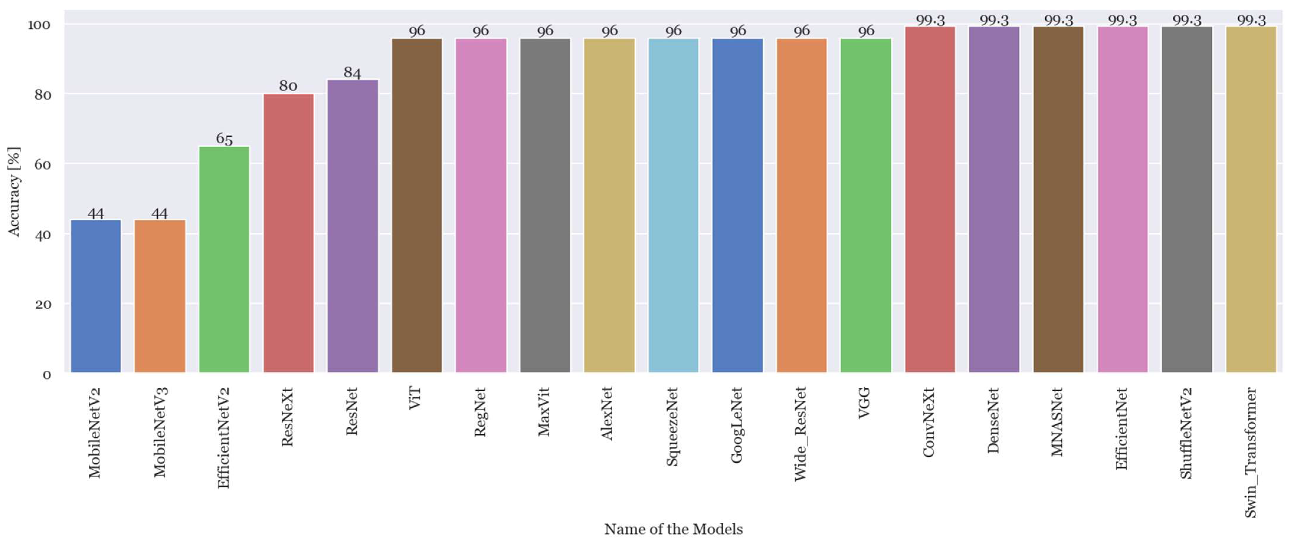
4.1. Experiment 1: Testing PyTorch Classification Architectures Using Different Combinations of Hyperparameters

In the initial experiment, the architectures available in the PyTorch framework were tested using different combinations of hyperparameters. All the executions were trained with a fixed batch size of four, 200 epochs, and 12 distinct parameter combinations in PyCharm. The objective was to identify the most effective model for vineyard flora classification. PyTorch has 20 available architectures; however, some of them have sub-architectures, giving a total of 80 [7]. As the combinations of hyperparameters provide 12 different simulations for each model, there is a total of 960 algorithms to run. However, some models were impossible to run due to the graphics of the computer because it did not have enough memory, especially Vit_l_16, Vit_l_32, Vit_h_14, and InceptionV3. Several models demonstrated high accuracy, with results ranging from 0% to 100%.

Figure 3 shows the best accuracies achieved by each model using the small and initial dataset. The values of accuracy presented correspond to the maximum value acquired in each architecture.

Figure 3. Highest accuracy achieved from all the architectures trained with the smallest dataset.

All the best accuracies achieved by each sub-architecture are shown in Table 1. The table is organized in the following order: name of the model, value of the learning rate, weight decay, number of layers, best validation accuracy, best test accuracy, and finally, the inference time in seconds (sec).

Table 1. Accuracy performance across PyTorch classification models.

N.	Models	Learning Rate	Weight Decay	N.er of Layers	Best Acc (%)	Test Accuracy (%)	Inference Time (sec)	N.	Models	Learning Rate	Weight Decay	N.er of Layers	Best Acc (%)	Test Accuracy (%)	Inference Time (sec)
1	MobileNetV2	0.0001	0.0001	Seq.	44.0	16.67	0.005	39	ShuffleNet_v2_x0_5	0.0001	0	Lin.	99.3	46.66	0.004
2	MobileNetV3_Large	0.0001	0	Lin.	44.0	16.67	0.006	40	ShuffleNet_v2_x1_0	0.001	0	Lin.	99.3	66.67	0.034
3	MobilenetV3_Small	0.001	0.0001	Seq.	44.0	26.67	0.005	41	ShuffleNet_v2_x1_5	0.001	0.0001	Lin.	99.3	16.67	0.005
4	MaxVit	0.001	0.0001	Lin.	96.0	76,67	0.055	42	ShuffleNet_v2_x2_0	0.001	0.0001	Lin.	96.0	66.67	0.005
5	AlexNet	0.0001	0	Seq.	96.0	33.33	0.001	43	EfficientNet_b0	0.001	0	Lin.	99.3	63.33	0.008
6	GoogLeNet	0.01	0	Lin.	96.0	10.00	0.007	44	EfficientNet_b1	0.0001	0	Lin.	99.3	86.66	0.010
7	Vit_b_16	0.0001	0	Seq.	96.0	56.67	0.006	45	EfficientNet_b2	0.001	0.0001	Seq.	99.3	50.00	0.011
8	Vit_b_32	0.0001	0.0001	Lin.	96.0	60	0.029	46	EfficientNet_b3	0.001	0	Lin.	99.3	60.00	0.012
9	ResNeXt50_32x4d	0.0001	0.0001	Lin.	80.0	13.33	0.006	47	EfficientNet_b4	0.001	0.0001	Lin.	99.3	73.33	0.014
10	ResNeXt101_32x8d	0.01	0.0001	Seq.	48.0	16.67	0.013	48	EfficientNet_b5	0.0001	0	Seq.	99.3	83.33	0.017
11	ResNeXt101_64x4d	0.0001	0.0001	Seq.	76.0	46.67	0.014	49	EfficientNet_b6	0.001	0	Lin.	99.3	23.33	0.020
12	ResNet18	0.0001	0	Lin.	84.0	43.33	0.002	50	EfficientNet_b7	0.001	0	Seq.	96.0	53.33	0.056
13	ResNet34	0.0001	0	Seq.	84.0	46.67	0.004	51	SqueezeNet1_0	0.0001	0	Lin.	96.0	20.00	0.034
14	ConvNeXt_Tiny	0.0001	0	Seq.	99.3	70.00	0.005	52	SqueezeNet1_1	0.0001	0	Lin.	96.0	46.67	0.002
15	ResNet50	0.0001	0	Lin.	80.0	43.33	0.021	53	VGG11	0.0001	0	Seq.	96.0	63.33	0.020
16	Convnext_small	0.001	0.0001	Lin.	99.3	26.67	0.038	54	RegNet_y_400mf	0.001	0	Seq.	96.0	66.66	0.022
17	Wide_ResNet50_2	0.0001	0.0001	Lin.	64.0	50.00	0.008	55	VGG11_bn	0.001	0	Lin.	96.0	63.33	0.034
18	Wide_ResNet101_2	0.0001	0	Seq.	96.0	33.33	0.014	56	RegNet_y_800mf	0.001	0	Seq.	96.0	56.66	0.032
19	Convnext_base	0.0001	0	Seq.	96.0	86.67	0.010	57	VGG_13	0.0001	0	Seq.	96.0	70.00	0.004
20	Convnext_large	0.0001	0	Seq.	96.0	90.00	0.041	58	RegNet_Y_1_6GF	0.001	0	Seq.	96.0	63.33	0.021
21	EfficientNet_v2_s	0.0001	0.0001	Seq.	65.0	20.00	0.015	59	VGG13_bn	0.0001	0	Seq.	96.0	76.67	0.004
22	EfficientNet_v2_m	0.0001	0.0001	Lin.	48.9	16.67	0.022	60	RegNet_y_3_2gf	0.001	0	Seq.	96.0	63.33	0.005
23	EfficientNet_v2_l	0.0001	0	Seq.	48.0	20.00	0.061	61	RegNet_y_8gf	0.001	0	Lin.	96.0	56.66	0.002
24	Swin_t	0.0001	0	Seq.	68.0	16.67	0.012	62	RegNet_y_16gf	0.001	0.0001	Lin.	96.0	53.33	0.034
25	Swin_s	0.0001	0	Seq.	72.0	20.00	0.024	63	VGG16	0.0001	0	Seq.	96.0	46.67	0.005
26	Swin_b	0.0001	0	Seq.	76.0	20.00	0.023	64	VGG16_bn	0.0001	0	Seq.	96.0	56.66	0.020
27	Swin_v2_t	0.0001	0	Seq.	99.3	36.67	0.016	65	VGG19	0.0001	0.0001	Lin.	96.0	46.67	0.004
28	Swin_v2_s	0.0001	0	Lin.	64.0	36.67	0.033	66	VGG19_bn	0.0001	0	Seq.	96.0	70.00	0.005
29	Swin_v2_b	0.0001	0	Seq.	72.0	26.67	0.031	67	RegNet_y_32gf	0.01	0	Lin.	96.0	46.67	0.004
30	DenseNet201	0.001	0	Seq.	96.0	20.00	0.034	68	RegNet_y_128gf	0.01	0.0001	Seq.	72.0	50.00	0.034
31	DenseNet161	0.01	0	Lin.	96.0	16.67	0.019	69	RegNet_x_400mf	0.001	0	Seq.	96.0	56.66	0.005
32	DenseNet169	0.01	0	Seq.	99.3	23.33	0.033	70	RegNet_x_800mf	0.001	0	Seq.	96.0	53.33	0.005
33	DenseNet121	0.01	0	Lin.	99.3	20.00	0.013	71	RegNet_x_1_6gf	0.001	0	Seq.	96.0	46.67	0.020
34	MNASNet0_5	0.001	0	Seq.	96.0	56.67	0.005	72	RegNet_x_3_2gf	0.01	0.0001	Lin.	96.0	50.00	0.004
35	MNASNet0_75	0.0001	0	Seq.	99.3	43.33	0.005	73	RegNet_x_8gf	0.01	0	Lin.	96.0	50.00	0.020
36	MNASNet1_0	0.0001	0.0001	Lin.	99.3	36.67	0.004	74	RegNet_x_16gf	0.01	0	Seq.	96.0	16.67	0.013
37	MNASNet1_3	0.0001	0	Seq.	96.0	40.00	0.005	75	RegNet_x_32gf	0.001	0	Lin.	96.0	33.33	0.018
38	ResNet101	0.0001	0	Lin.	96.0	20.00	0.004	76	ResNet152	0.0001	0	Seq.	96.0	16.67	0.0005

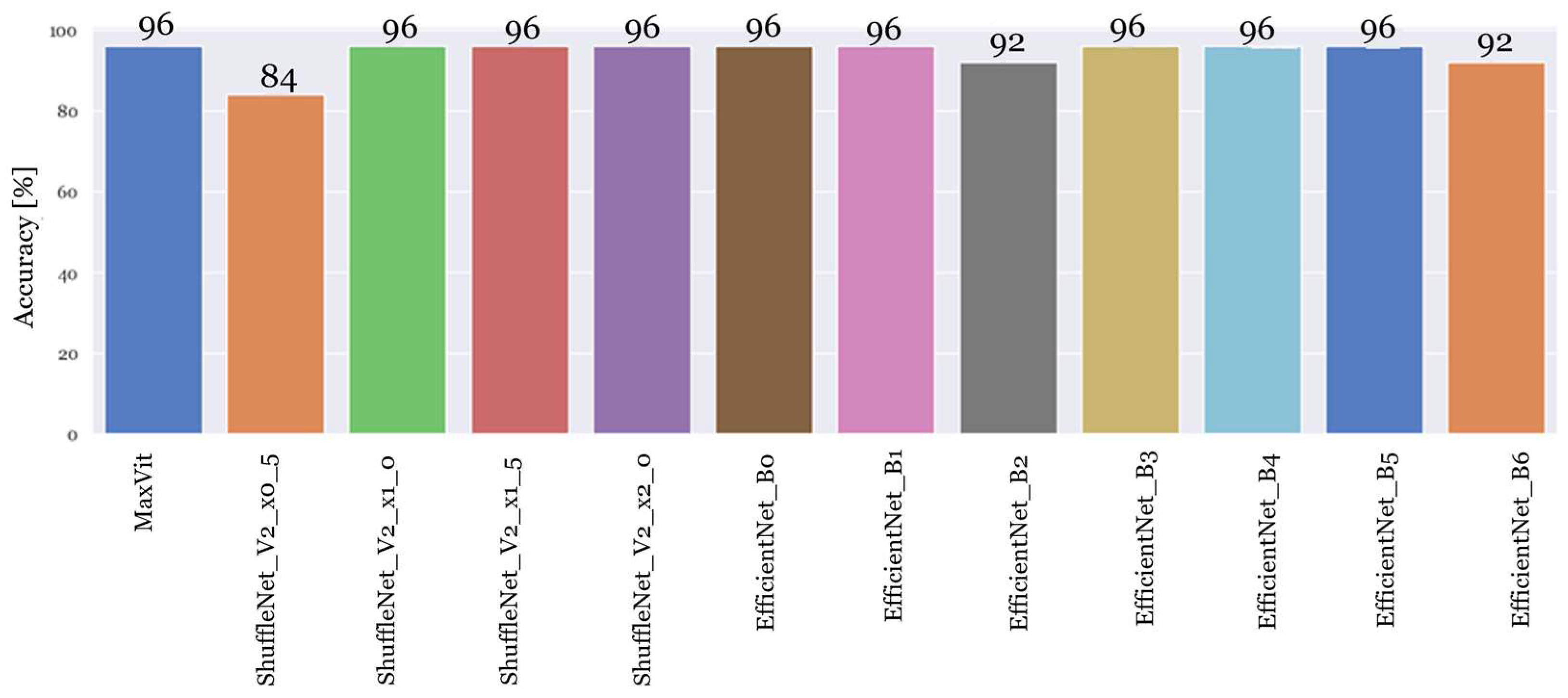
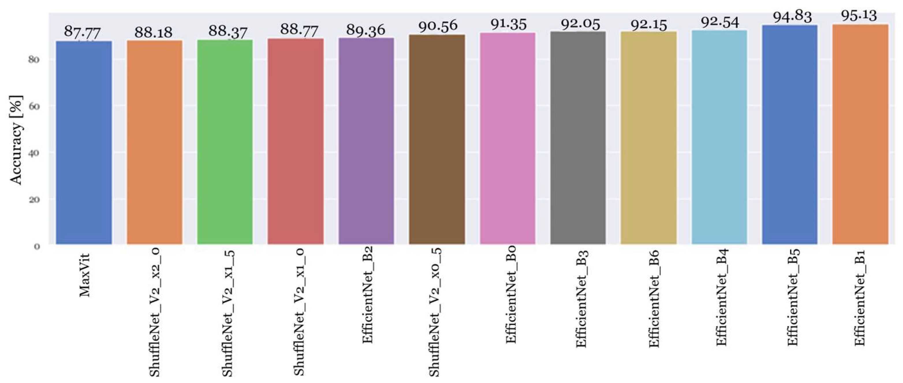
4.2. Experiment 2: Testing the Best-Performing PyTorch Classification Architectures

In the second experiment, only the best-performing models, namely, MaxVit, ShuffleNetV2, and EfficientNet, were further simulated. The analysis of the results of these architectures indicated that 25 epochs were sufficient to achieve optimal results. Therefore, the twelve models were trained using the same dataset, the same combination of hyperparameters, and a reduced training period of 25 epochs instead of the initial 200.

The outcomes of these experiments for each model can be found in Figure 4.

Figure 4. Performance evaluation of the top twelve sub-architectures: simulation results for 25 epochs.

4.3. Experiment 3: Testing a New Dataset with Re-Trained PyTorch Classification Architectures

Smaller datasets, such as the initial one of 172 images, pose challenges for training complex deep learning models. Such models require large data to generalize effectively, and with limited data, overfitting risks increase. For smaller datasets, overly complex architectures might not be suitable, as they demand extensive data for effective training. So, in this phase of the research, the twelve architectures were re-trained using the initial combination of hyperparameters that yielded the best results and the new dataset, extending the simulation to 200 epochs. The aim was to assess whether these models could maintain their performance when trained with varying quantities of images and more variance in the backgrounds. The updated dataset was obtained by downloading several images from various platforms, including Flora-On [37], INaturalist [38], UTAD Botanical Garden [39], and the Global Biodiversity Information Facility (GBIF) [40]. This dataset comprises 6730 images categorized into the five classes that were defined in the dataset. The images were randomly split, following the standard practice of an 85% training set and a 15% validation set, as recommended in the literature [33]. Consequently, 5724 images were used for training, while 1006 photos were reserved for model validation. The distribution of these images across different species in both the training and validation sets is shown in Figure 5.

Figure 5. The extended dataset of 6730 images is visually represented, showcasing the distribution of images for training and validation across different species. The blue line indicates the number of training images per species, and the orange line represents the validation images. In comparison, the green line shows training images and the red line depicts validation images from the initial dataset.

Figure 6 shows the results of the accuracy of the top twelve models trained with the new and extended dataset.

Figure 6. Model performance of the top twelve models trained with the extended dataset.

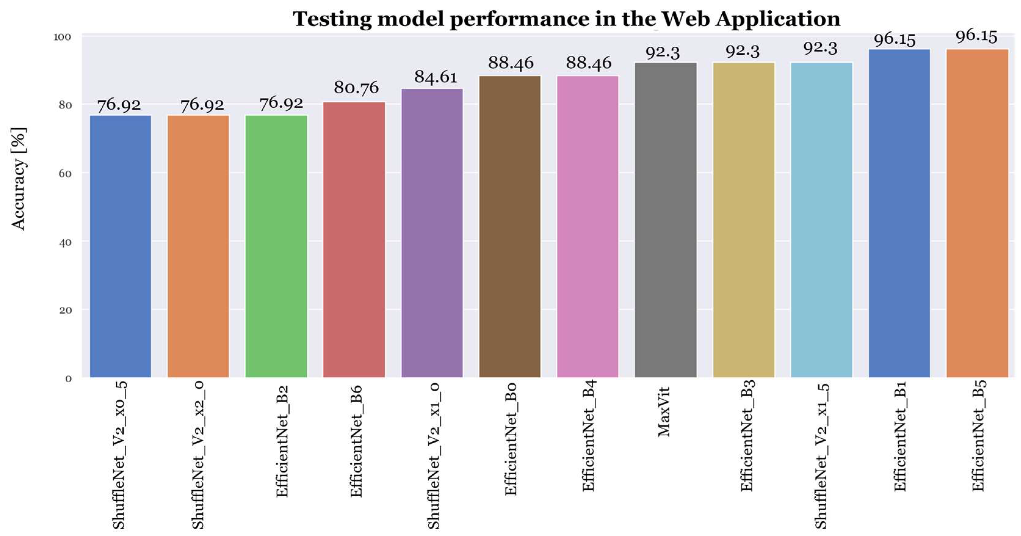
4.4. Experiment 4: Testing Best-Performing Models of PyTorch Classification Architectures with New Images

To evaluate the models, a web application was developed using Gradio [41]. New testing images were captured (26 images) in the field, with the same camera used in experiment 1, after completing all training and experiments, averaging five images per species. These images were taken using a phone camera for further assessment.

During this phase, images of the five plant species were sequentially uploaded to the web application’s interface, and their classifications were verified.

In the testing stage, the MaxVit model and various versions of ShuffleNet and EfficientNet, which were utilized in previous sections, were employed. Each model was tested with the same test images.

Users can upload an image of a plant species, request its classification, and receive the species’ name in return.

The results, shown in Figure 7, show that both EfficientNet_B5 and EfficientNet_B1 achieved superior accuracy.

Figure 7. Model performance of the top twelve models after the testing phase.

5. Discussion of Results

The following findings and challenges can be determined by the results of the actual tests.

The first experiment effectively found both the ideal hyperparameter combination and the top-performing simulated models. A default weight decay setting was utilized in 56 instances, while a variable weight decay was selected in 20 cases. Sequential fully connected layers outperformed linear configurations in 42 instances out of 76 tests. The selection of hyperparameters such as learning rate, weight decay, and layer configuration significantly influences model performance. Lower learning rates, such as 0.0001, contribute to stable convergence and prevent the overshooting of optimal solutions. Default weight decay (with a value of zero) served as effective regularization, enhancing model generalization. Sequential fully connected layers proved efficient in capturing complex patterns and relationships in the data [34,35,36].

According to the results, the three architectures were chosen as the better ones and used in the following experiments. The study identified MaxVit, ShuffleNet, and EfficientNet as superior models. Despite MaxVit only reaching a maximum accuracy of 96%, this architecture was chosen because it achieved this accuracy value during several epochs and repeated the process in several tests with different combinations of hyperparameters. On the other hand, the other architectures that achieved an accuracy of 99.3%, such as ConvNeXt_Tiny, Convnext_small, Swin_v2_t, DenseNet121, DenseNet169, MNASNet0_75, and MNASNet1_0, were not considered the best because they reached their maximum in a lower number of epochs than MaxVit and fewer tests with different hyperparameter configurations. The three architectures achieved a high accuracy and good results over the 200 epochs, and they were the ones that achieved this accuracy more times over the 12 combinations. These models distinguished themselves through innovative, resource-efficient designs, leveraging available resources optimally and striking a balance between depth and complexity. The fine-tuning of hyperparameters and high-quality, meticulously labeled data were crucial contributors to their success [18,19].

According to the inference times, some images take only a few seconds (e.g., 0.001 s), while others might take longer (e.g., 0.055 s). Inference times that differ plenty may indicate that some images are more difficult or time-consuming for the model to process. Despite this, all the inference timings were less than one second. However, the sub-architectures’ average time inside the same architectures was consistent, indicating a stable performance.

In the second experiment, the ShuffleNet_v2_x0_5 model exhibited the lowest accuracy at 84%, followed by EfficientNet_B2 and EfficientNet_B6 with an accuracy of 92%. The rest of the models achieved a maximum accuracy of 96%.

With only 25 epochs, these models might not have had enough time to converge to an optimal solution. It is recommended to extend the training duration by increasing the number of epochs, allowing these models a better opportunity to converge and extract valuable insights from the dataset [42].

For the third experiment, it is possible to conclude that with a larger dataset, these three models achieved very good accuracy as well. However, it reached accuracy values slightly lower than the original dataset that was developed for this purpose. These disparities can introduce different complexities for the models, potentially posing a slightly greater challenge in achieving the same level of accuracy [43]. Furthermore, it is possible to distinguish EfficientNetB1 from the other models.

The larger dataset may have unique characteristics and variations compared to the smaller dataset, introducing complexities for models. The larger dataset offers a more diverse array of examples, making it more challenging for models to overfit. Hyperparameters used in the smaller dataset may not be optimally suited for the larger dataset, and the distribution of classes or patterns may differ. Data quality issues within the new dataset can also lead to diminished accuracy. However, training on extensive distributed computing systems with abundant data and computational resources can improve model resilience and adaptability to real-world applications [43,44].

Finally, in the last experiment, during the test phase, Centaurea melitensis was often mistaken for Erodium moschatum, while Echium Plantagineum was frequently categorized as Erodium moschatum due to its leaf and flower similarities. Lolium rigidum’s misclassifications were attributed to training errors, as it lacked similarities with other species. Ornithopus compressus was occasionally misclassified as Centaurea melitensis due to shared yellow flowers.

6. Conclusions

This paper discusses the use of AI in agriculture to fight unwanted flora. ML algorithms are employed to identify and manage unnecessary flora, addressing economic and environmental threats. The research focuses on testing NN models and hyperparameters for plant classification optimizing architectures and training methods to achieve the best accuracy possible. The study contributes to sustainable agriculture by reducing pesticide use, automating weed classification, and minimizing manual labor. Three stand-out models, MaxVit, ShuffleNet, and EfficientNet, achieved a maximum accuracy of 96%, 99.3%, and 99.3%, respectively, in the first group of experiments. In the second experiment, these elevated accuracies were maintained at 96% for all three models. However, in the third experiment, where an extended dataset was tested, the models EfficientNet_B1 and EfficientNet_B5 stood out, reaching 95.13% and 94.83%, respectively. These two models once again proved their high accuracy in the fourth experiment, where they both achieved an accuracy of 96.15%. The research demonstrates the effectiveness of these algorithms and highlights the potential of AI and ML to address real-world challenges in agriculture.

References

1. Hasan, A.S.M.M.; Sohel, F.; Diepeveen, D.; Laga, H.; Jones, M.G.K. A survey of deep learning techniques for weed detection from images. Comput. Electron. Agric. 2021, 184, 106067. [Google Scholar] [CrossRef]
2. MacLaren, C.; Storkey, J.; Menegat, A.; Metcalfe, H.; Dehnen-Schmutz, K. An ecological future for weed science to sustain crop production and the environment. A review. Agron. Sustain. Dev. 2020, 40, 24. [Google Scholar] [CrossRef]
3. Dyrmann, M.; Karstoft, H.; Midtiby, H.S. Plant species classification using deep convolutional neural network. Biosyst. Eng. 2016, 151, 72–80. [Google Scholar] [CrossRef]
4. Shaikh, T.A.; Rasool, T.; Rasheed Lone, F. Towards leveraging the role of machine learning and artificial intelligence in precision agriculture and smart farming. Comput. Electron. Agric. 2022, 198, 107119. [Google Scholar] [CrossRef]
5. Paszke, A.; Gross, S.; Massa, F.; Lerer, A.; Bradbury, J.; Chanan, G.; Killeen, T.; Lin, Z.; Gimelshein, N.; Antiga, L.; et al. PyTorch: An imperative style, High-performance Deep Learning library. arXiv 2019, arXiv:1912.01703. [Google Scholar]
6. Lv, Q.; Zhang, S.; Wang, Y. Deep Learning model of image classification using Machine Learning. Adv. Multimed. 2022, 2022, 3351256. [Google Scholar] [CrossRef]
7. Models and Pre-Trained Weights—Torchvision 0.16 Documentation. Available online: https://pytorch.org/vision/stable/models.html#classification (accessed on 30 October 2023).
8. Rahman, A.; Lu, Y.; Wang, H. Performance evaluation of deep learning object detectors for weed detection for cotton. Smart Agric. Technol. 2023, 3, 100126. [Google Scholar] [CrossRef]
9. Simonyan, K.; Zisserman, A. very deep convolutional networks for large-scale image recognition. arXiv 2015, arXiv:1409.1556. [Google Scholar]
10. Ma, N.; Zhang, X.; Zheng, H.-T.; Sun, J. ShuffleNet V2: Practical guidelines for efficient CNN architecture design. arXiv 2018, arXiv:1807.11164. [Google Scholar]
11. Radosavovic, I.; Kosaraju, R.P.; Girshick, R.; He, K.; Dollár, P. Designing network design spaces. arXiv 2020, arXiv:2003.13678. [Google Scholar]
12. Szegedy, C.; Vanhoucke, V.; Ioffe, S.; Shlens, J.; Wojna, Z. Rethinking the inception architecture for computer vision. arXiv 2015, arXiv:1512.00567. [Google Scholar]
13. Boesch, G. Deep Residual Networks (ResNet, ResNet50)—2023 Guide. viso.ai, 1 January 2023. Available online: https://viso.ai/deep-learning/resnet-residual-neural-network/ (accessed on 28 February 2023).
14. Xie, S.; Girshick, R.; Dollár, P.; Tu, Z.; He, K. Aggregated residual transformations for deep neural networks. arXiv 2017, arXiv:1611.05431. [Google Scholar]
15. Zagoruyko, S.; Komodakis, N. Wide residual networks. arXiv 2017, arXiv:1605.07146. [Google Scholar]
16. Dosovitskiy, A.; Beyer, L.; Kolesnikov, A.; Weissenborn, D.; Zhai, X.; Unterthiner, T.; Dehghani, M.; Minderer, M.; Heigold, G.; Gelly, S.; et al. An Image is worth 16x16 words: Transformers for image recognition at scale. arXiv 2021, arXiv:2010.11929. [Google Scholar]
17. Liu, Z.; Lin, Y.; Cao, Y.; Hu, H.; Wei, Y.; Zhang, Z.; Lin, S.; Guo, B. Swin Transformer: Hierarchical vision transformer using shifted windows. arXiv 2021, arXiv:2103.14030. [Google Scholar]
18. Tu, Z.; Talebi, H.; Zhang, H.; Yang, F.; Milanfar, P.; Bovik, A.; Li, Y. MaxViT: Multi-axis vision transformer. arXiv 2022, arXiv:2204.01697. [Google Scholar]
19. Liu, H.; Yao, D.; Yang, J.; Li, X. Lightweight Convolutional Neural Network and its application in rolling bearing fault diagnosis under variable working conditions. Sensors 2019, 19, 4827. [Google Scholar] [CrossRef]
20. Tan, M.; Le, Q.V. EfficientNet: Rethinking model scaling for Convolutional Neural Networks. arXiv 2020, arXiv:1905.11946. [Google Scholar]
21. Alibabaei, K.; Gaspar, P.D.; Lima, T.M.; Campos, R.M.; Girão, I.; Monteiro, J.; Lopes, C.M. A review of the challenges of using deep learning algorithms to support decision-making in agricultural activities. Remote Sens. 2022, 14, 638. [Google Scholar] [CrossRef]
22. Alibabaei, K.; Gaspar, P.D.; Assunção, E.; Alirezazadeh, S.; Lima, T.M. Irrigation optimization with a deep reinforcement learning model: Case study on a site in Portugal. Agric. Water Manag. 2022, 263, 107480. [Google Scholar] [CrossRef]
23. Andrea, C.-C.; Daniel, B.B.M.; Jose Misael, J.B. Precise weed and maize classification through convolutional neuronal networks. In Proceedings of the 2017 IEEE Second Ecuador Technical Chapters Meeting (ETCM), Salinas, Ecuador, 16–20 October 2017; IEEE: Piscataway, NJ, USA, 2017; pp. 1–6. [Google Scholar] [CrossRef]
24. Gao, J.; Nuyttens, D.; Lootens, P.; He, Y.; Pieters, J.G. Recognising weeds in a maize crop using a random forest machine-learning algorithm and near-infrared snapshot mosaic hyperspectral imagery. Biosyst. Eng. 2018, 170, 39–50. [Google Scholar] [CrossRef]
25. Bakhshipour, A.; Jafari, A. Evaluation of support vector machine and artificial neural networks in weed detection using shape features. Comput. Electron. Agric. 2018, 145, 153–160. [Google Scholar] [CrossRef]
26. Sa, I.; Chen, Z.; Popovic, M.; Khanna, R.; Liebisch, F.; Nieto, J.; Siegwart, R. weedNet: Dense semantic weed classification using multispectral images and MAV for smart farming. IEEE Robot. Autom. Lett. 2018, 3, 588–595. [Google Scholar] [CrossRef]
27. Yang, X.; Ye, Y.; Li, X.; Lau, R.Y.K.; Zhang, X.; Huang, X. Hyperspectral image classification with deep learning models. IEEE Trans. Geosci. Remote Sens. 2018, 56, 5408–5423. [Google Scholar] [CrossRef]
28. Yashwanth, M.; Chandra, M.L.; Pallavi, K.; Showkat, D.; Kumar, P.S. Agriculture automation using deep learning methods implemented using Keras. In Proceedings of the 2020 IEEE International Conference for Innovation in Technology (INOCON), Bangluru, India, 6–8 November 2020; IEEE: Piscataway, NJ, USA, 2020; pp. 1–6. [Google Scholar] [CrossRef]
29. Jin, X.; Che, J.; Chen, Y. Weed identification using deep learning and image processing in vegetable plantation. IEEE Access 2021, 9, 10940–10950. [Google Scholar] [CrossRef]
30. El-Kenawy, E.-S.M.; Khodadadi, N.; Mirjalili, S.; Makarovskikh, T.; Abotaleb, M.; Karim, F.K.; Alkahtani, H.K.; Abdelhamid, A.A.; Eid, M.M.; Horiuchi, T.; et al. Metaheuristic optimization for improving weed detection in wheat images captured by drones. Mathematics 2022, 10, 4421. [Google Scholar] [CrossRef]
31. Sunil, G.C.; Koparan, C.; Ahmed, M.R.; Zhang, Y.; Howatt, K.; Sun, X. A study on deep learning algorithm performance on weed and crop species identification under different image background. Artif. Intell. Agric. 2022, 6, 242–256. [Google Scholar] [CrossRef]
32. Sunil, G.C.; Zhang, Y.; Koparan, C.; Ahmed, M.R.; Howatt, K.; Sun, X. Weed and crop species classification using computer vision and deep learning technologies in greenhouse conditions. J. Agric. Food Res. 2022, 9, 100325. [Google Scholar] [CrossRef]
33. Solawetz, J. Train, Validation, Test Split for Machine Learning. Roboflow Blog. Available online: https://blog.roboflow.com/train-test-split/ (accessed on 24 August 2023).
34. Brownlee, J. Difference between A Batch and an Epoch in a Neural Network. Available online: https://machinelearningmastery.com/difference-between-a-batch-and-an-epoch/ (accessed on 28 August 2023).
35. Nabi, J. Hyper-Parameter Tuning Techniques in Deep Learning. Medium. Available online: https://towardsdatascience.com/hyper-parameter-tuning-techniques-in-deep-learning-4dad592c63c8 (accessed on 28 August 2023).
36. Zhao, G.; Liu, G.; Fang, L.; Tu, B.; Ghamisi, P. Multiple convolutional layers fusion framework for hyperspectral image classification. Neurocomputing 2019, 339, 149–160. [Google Scholar] [CrossRef]
37. Flora-On|Flora de Portugal. Available online: https://flora-on.pt/ (accessed on 19 April 2023).
38. Uma Comunidade Para Naturalistas · iNaturalist. Available online: https://www.inaturalist.org/ (accessed on 9 September 2023).
39. Jardim Botânico UTAD. Available online: https://jb.utad.pt (accessed on 9 September 2023).
40. GBIF. Available online: https://www.gbif.org/ (accessed on 9 September 2023).
41. Gradio: UIs for Machine Learning. Available online: https://gradio.app (accessed on 21 September 2023).
42. Unzueta, D. Convolutional Layers vs. Fully Connected Layers. Medium. Available online: https://towardsdatascience.com/convolutional-layers-vs-fully-connected-layers-364f05ab460b (accessed on 23 September 2023).
43. Kapoor, R.; Sharma, D.; Gulati, T. State of the art content based image retrieval techniques using deep learning: A survey. Multimed. Tools Appl. 2021, 80, 29561–29583. [Google Scholar] [CrossRef]
44. Taye, M.M. Understanding of machine learning with deep learning: Architectures, workflow, applications and future directions. Computers 2023, 12, 91. [Google Scholar] [CrossRef]