Computing RF Tree Distance over Succinct Representations

Abstract

There are several tools available to infer phylogenetic trees, which depict the evolutionary relationships among biological entities such as viral and bacterial strains in infectious outbreaks or cancerous cells in tumor progression trees. These tools rely on several inference methods available to produce phylogenetic trees, with resulting trees not being unique. Thus, methods for comparing phylogenies that are capable of revealing where two phylogenetic trees agree or differ are required. An approach is then proposed to compute a similarity or dissimilarity measure between trees, with the Robinson–Foulds distance being one of the most used, and which can be computed in linear time and space. Nevertheless, given the large and increasing volume of phylogenetic data, phylogenetic trees are becoming very large with hundreds of thousands of leaves. In this context, space requirements become an issue both while computing tree distances and while storing trees. We propose then an efficient implementation of the Robinson–Foulds distance over tree succinct representations. Our implementation also generalizes the Robinson–Foulds distances to labelled phylogenetic trees, i.e., trees containing labels on all nodes, instead of only on leaves. Experimental results show that we are able to still achieve linear time while requiring less space. Our implementation in C++ is available as an open-source tool.

1. Introduction

Comparative evaluation of differences, similarities, and distances between phylogenetic trees is a fundamental task in computational phylogenetics [1]. There are several measures for assessing differences between two phylogenetic trees, some of them based on rearrangements, others based on topology dissimilarity and in this case, some of them take also into account the branch length [2]. The rearrangement measures are based on finding the minimum number of rearrangement steps required to transform one tree into the other. Possible rearrangement steps include nearest-neighbor interchange (NNI), subtree pruning and regrafting (SPR), and tree bisection and reconnection (TBR). Unfortunately, such measures are seldom used in practice for large studies as they are expensive to calculate in general. NP completeness has been shown for distances based on NNI [3], TBR [4], and SPR [5]. Measures based on topological dissimilarity are commonly used. One of the most used is the topological distance of Robinson and Foulds [6] (RF) and its branch length variation [7]. RF-like distances, when applied to rooted trees, are all based on the idea of shared clades, i.e., specific kinds of subtrees (for rooted trees) or branches defined by possession of exactly the same tips (the leaves of the tree). Namely, it quantifies the dissimilarity between two trees based on the differences in their clades for rooted trees or bipartitions if applied to unrooted trees. Formally, a clade or cluster $C\left(n\right)$ of a tree T is defined by the set of leaves (or nodes in fully labelled trees) that are a descendant from a particular internal node n.

Alternative methods or variants have been considered such as Triples distance [8], tree alignment metric [9], nodal or path distance [10,11], Quartet method of Estabrook et al. [12], ‘Generalized’ Robinson–Foulds metrics [13], Geodesic distance [14,15], Generalized Robinson–Foulds distance [16], which is not equivalent to Robinson–Foulds distance, among others. Some of these measures were generalized for phylogenetic networks, and new measures were also proposed [17]. It is common to use more than one measure to compare phylogenetic trees or networks. Clearly, the best measure depends on the dataset, and there are studies such as [2] that offer practical recommendations for choosing tree distance measures in different applications. More generally, measures may benefit certain properties over others, i.e., they have different discriminatory power [18].

The computation of the RF distance can be achieved in linear time and space. A linear time algorithm for calculating the RF distance was first proposed by Day [19]. It efficiently determines the number of bipartitions or clades that are present in one tree but not in the other. Furthermore, there have been advancements in the computation of the RF distance that achieve sublinear time complexity; Pattengale et al. [20] introduced an algorithm that can compute an approximation of the RF distance in sublinear time. However, it is important to note that the sublinear algorithm is not exact and may introduce some degree of error in the computed distances. Recently, a linear time and space algorithm [21] was proposed that addresses the labelled Robinson–Foulds (RF) distance problem, considering labels assigned to both internal and leaf nodes of the trees. However, their distance is based on edit distance operations applied to nodes and thus do not produce the exact RF value. Moreover, implementation is based on the Day algorithm [19].

Considering, however, the increasingly large volume of phylogenetic data [22], the size of phylogenetic trees has grown substantially, often consisting of hundreds of thousands of leaf nodes. This poses significant challenges in terms of space requirements for computing tree distances, or even for storing trees. Hence, we propose an efficient implementation of the Robinson–Foulds distance over succinct representations of trees [23]. Our implementation not only addresses the standard Robinson–Foulds distance, but it also extends it to handle fully labelled and weighted phylogenetic trees. By leveraging succinct representations, we are able to achieve practical linear time while significantly reducing space requirements. Experimental results demonstrate the effectiveness of our implementation in spite of expected trade-offs on running time overhead versus space requirements due to the use of succinct data structures.

The structure of this paper is as follows. In Section 2, we introduce each type of phylogenetic trees that are considered in this paper, providing illustrative examples, the Robinson–Foulds metric and some variants, as well as the Newick format. Then, in Section 3, we describe how to use succint data structures to represent these phylogenetic trees, the operations to manage this representation for this context, as well as the algorithms to compute the Robinson–Foulds metrics and considered variants. In Section 4, we depict implementation details. Then, in Section 5, we present and discuss experimental evaluation of our approach. Finally, in Section 6, we conclude and present future issues.

2. Background

A phylogenetic tree, denoted as $T=(V,E)$, is defined as a connected acyclic graph. The set V, also denoted as $V\left(T\right)$, represents the vertices (nodes) of tree T. The set $E\subseteq V\times V$, also denoted as $E\left(T\right)$, represents the edges (links) of tree T. The leaves of the tree, which are the vertices of degree one, are labelled with data that represent species, strains or even genes. A phylogenetic tree represents then the evolutionary relationships among taxonomical groups, or taxa.

In most phylogenetic inference methods, the internal vertices of the tree represent hypothetical or inferred common ancestors of the entities represented by the leaves. These internal vertices do not typically have a specific label or represent direct data. However, there are some distance based phylogenetic inference methods that infer a fully labelled phylogenetic tree [24]. In such cases, the internal vertices may also have labels associated with them, providing additional information about the inferred common ancestors. We denote the labels of a phylogetic tree T by $L\left(T\right)$. The inferred phylogenetic trees can be rooted or unrooted, depending on whether or not a specific root node is assigned. In the rooted ones, there exists a distinguished vertex called the root of T.

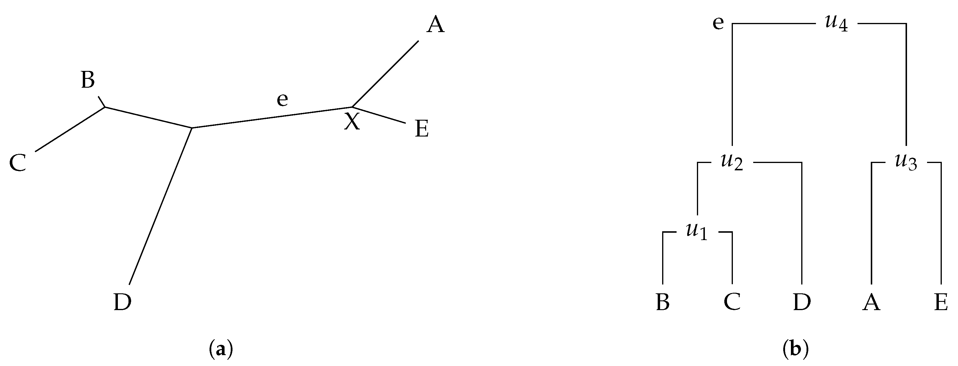
To calculate the Robinson–Foulds (RF) distance on a rooted or unrooted tree, comparison of the clades or bipartitions of the trees is needed, respectively. As mentioned before, a clade is a group on a tree that includes a node and all of the lineages descended from that node. Thus, clades can be seen as the subtrees of a phylogenetic tree. A bipartition of a tree is induced by edge removal  [1]. Nevertheless, we can convert an unrooted tree into a rooted one by adding an arbitrary root node [25] (see Figure 1). A measure based on Robison–Foulds distance to compare unrooted with rooted trees was also proposed [26]. In this work, we consider rooted trees.

Let T be a rooted tree. A sub-tree S of T, which we denote by $S\left(T\right)$, is a tree such that $V\left(S\right)\subseteq V\left(T\right)$, $E\left(S\right)\subseteq E\left(T\right)$, and the endpoints of any edge in $E\left(S\right)$ must belong to $V\left(S\right)$. We denote by $T\left(v\right)$ the maximum sub-tree of T that is rooted at v. Thus, for each $v\in V\left(T\right)$, we define the cluster at v in T as $c\left(v\right)=L\left(T\right(v\left)\right)$. For instance, the rooted tree in Figure 1 contains nine clusters, namely $c\left(B\right)=\left\{B\right\}$, $c\left(C\right)=\left\{C\right\}$, $c\left(D\right)=\left\{D\right\}$, $c\left(A\right)=\left\{A\right\}$, $c\left(E\right)=\left\{E\right\}$, $c\left(u_1\right)=\{B,C\}$, $c\left(u_2\right)=\{B,C,D\}$, $c\left(u_3\right)=\{A,E\}$ and $c\left(u_4\right)=\{B,C,D,A,E\}$, with $u_i$ denoting unnamed or unlabelled nodes in T. We notice that nodes labelled by symbol u represent hypothetical taxonomic units and thus they are not included on the cluster. The set of all clusters present in T is denoted by $C\left(T\right)$, i.e., $C\left(T\right)={\cup }_{v\in V\left(T\right)}\left\{c\left(v\right)\right\}$. In Figure 1, $C\left(T_1\right)$ contains the previous nine clusters. The Robison–Foulds distance measures the dissimilarity between two trees by counting the differences in the clades they contain if rooted.

Definition 1 

(Robison and Foulds, 1981 [6]). The Robinson–Foulds (RF) distance between two rooted trees $T_1$ and $T_2$, with unique labelling in leaves, is defined by

$$RF(T_1,T_2)=|C\left(T_1\right)\setminus C\left(T_2\right)| \cup |C\left(T_2\right)\setminus C\left(T_1\right)|.$$

We notice that this definition is equivalent to $RF(T_1,T_2)=|C\left(T_1\right)|+|C\left(T_2\right)|-2|C\left(T_1\right)\cap C\left(T_2\right)|$, commonly found in the literature. We also note that most software implementations usually divide the RF distance by 2 [2], and further normalize it.

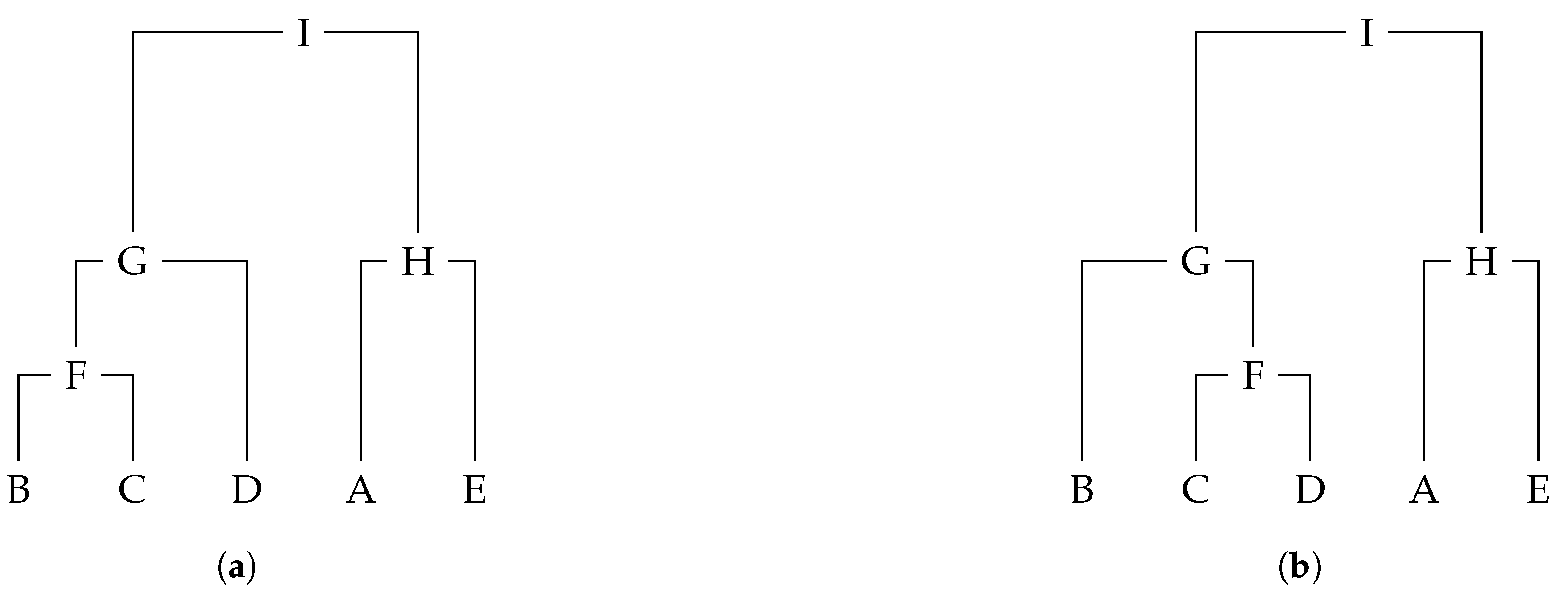
When dealing with fully labelled phylogenetic trees, labels are present not only in leaves but also in internal nodes. Figure 2 depicts two rooted and fully labelled phylogenetic trees. The clusters of tree $T_2$ are $C\left(A\right)=\left\{A\right\}$, $C\left(B\right)=\left\{B\right\}$, $C\left(C\right)=\left\{C\right\}$, $C\left(D\right)=\left\{D\right\}$, $C\left(E\right)=\left\{E\right\}$, $C\left(F\right)=\{B,C,F\}$, $C\left(G\right)=\{B,C,F,D,G\}$, $C\left(H\right)=\{A,E,H\}$ and $C\left(I\right)=\{B,C,F,D,G,A,E,H,I\}$. The RF distance given in Definition 1 can be extended to fully labelled trees by just noting that, given $v\in V\left(T\right)$, $c\left(v\right)=L\left(T\right(v\left)\right)$ includes now the labels of all nodes in subtree $T\left(v\right)$; and hence the clusters in $C\left(T\right)$ include the labels for all nodes as well.

Definition 2. 

The extended Robinson–Foulds (RF) distance between two fully labelled rooted trees $T_1$ and $T_2$, with unique labelling in all nodes, is defined by

$$eRF(T_1,T_2)=|C\left(T_1\right)\setminus C\left(T_2\right)| \cup |C\left(T_2\right)\setminus C\left(T_1\right)|.$$

Let us consider trees $T_2$ and $T_3$ in Figure 2; $eRF(T_2,T_3)=2$ since there are only two distinct clusters in $T_2$ and $T_3$, namely $\{B,C,F\}$ and $\{C,D,F\}$.

Even though RF can offer a very reliable distance between two trees in terms of their topology, sometimes it is convenient to consider weights. A version of Robinson–Foulds distance for weighted trees (wRF) takes then into account the branch weights of both trees [7]. These weights represent, for instance, the varying levels of correction for DNA sequencing errors. We let T be a phylogenetic rooted tree, $v\in V\left(T\right)$, $w:E\left(T\right)\to \mathbf{R}$, $e\in E\left(T\right)$ the edge with target v, and $c\left(v\right)$ the cluster at v in T as before; the weight of cluster $c\left(v\right)$ in T, $w_T\left(c\left(v\right)\right)$ is defined as $w\left(e\right)$.

Definition 3 

(Robison and Fould, 1979 [7]). The weighted Robinson–Foulds (wRF) distance between two rooted trees $T_1$ and $T_2$, with unique labelling in leaves, is defined as

$$wRF(T_1,T_2)=\sum _{c\in C\left(T_1\right)\cap C\left(T_2\right)}|w_{T_1}\left(c\right)-w_{T_2}\left(c\right)|+\sum _{c\in C\left(T_1\right)\setminus C\left(T_2\right)}{w}_{T_1}\left(c\right)+\sum _{c\in C\left(T_2\right)\setminus C\left(T_1\right)}{w}_{T_2}\left(c\right).$$

In fact, at lower levels of sequencing error, RF distance usually exhibits a consistent pattern, showcasing the superiority of proper correction for both over- and undercorrection for DNA sequencing error. Interestingly, in this context, correction had no impact on RF scores. Conversely, at extremely high levels of sequencing error, wRF results suggested that proper correction and overcorrection were equivalent, while the RF scores demonstrated that overcorrection led to the destruction of topological recovery. Then, both measures complement themselves [2]. Definition 4 extends wRF to labelled rooted phylogenetic trees assuming the extension of $c\left(v\right)$ and $C\left(T\right)$ as before.

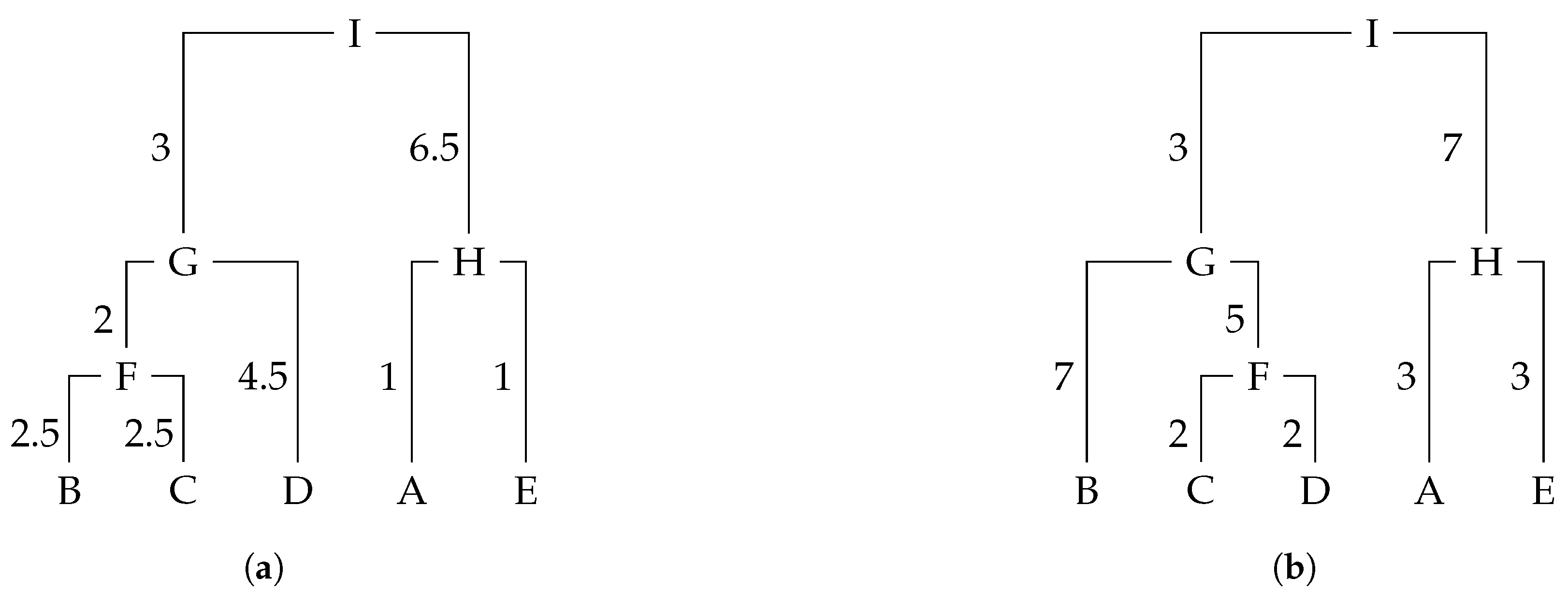
Definition 4. 

The weighted labelled Robinson–Foulds (weRF) distance between two fully labelled rooted trees $T_1$ and $T_2$, with unique labelling in all nodes, is defined as follows:

$$weRF(T_1,T_2)=\sum _{c\in C\left(T_1\right)\cap C\left(T_2\right)}|w_{T_1}\left(c\right)-w_{T_2}\left(c\right)|+\sum _{c\in C\left(T_1\right)\setminus C\left(T_2\right)}{w}_{T_1}\left(c\right)+\sum _{c\in C\left(T_2\right)\setminus C\left(T_1\right)}{w}_{T_2}\left(c\right).$$

Let us consider trees $T_2$ and $T_3$ in Figure 3; $wRF(T_2,T_3)=19$.

Phylogenetic trees are commonly represented and stored using the well-known Newick tree format. For instance, the rooted tree in Figure 1 can be represented as (((B, C), D),(A, E));. In this example, we only have labels on the leaves and we do not have edge weights. The Newick format also supports edge weights. For instance, in Figure 3, tree $T_2$ can be represented as (((B:2.5,C:2.5):2,D:4.5):3,(A:1,E:1):6.5);. Moreover, the newick format also supports internal labelled vertices and edge weights, e.g., (((B:0.2, C:0.2)W:0.3, D:0.5)X:0.6, (A:0.5, E:0.5)Y:0.6)Z;. Thus, it is common that tools that compute the RF distance support as input trees in the Newick format. We notice also that some phylogenetic inference algorithms may produce nary phylogenetic trees, such is the case, for instance, of goeBURST [27] or MSTree V2 [28].

3. Methodology

Our approach consists in using succinct data structures, namely encoding each tree using balanced parentheses and represent it as a bit vector. Each tree is then represented by a bit vector of size $2n$ bits, where n is the number of nodes present in the tree. This space is further increased by $o\left(n\right)$ bits to support efficiently primitive operations over the bit vector [29]. For comparing trees, we need to also store the label permutation corresponding to each tree. Each permutation can be represented in $(1+\epsilon )nlogn$ bits while answering permutation queries in constant time and inverse permutation queries in $O(1/\epsilon )$ time [23]. Hence, each tree with n nodes can be represented in $2n+o\left(n\right)+(1+\epsilon )nlogn$ bits.

3.1. Balanced Parentheses Representation

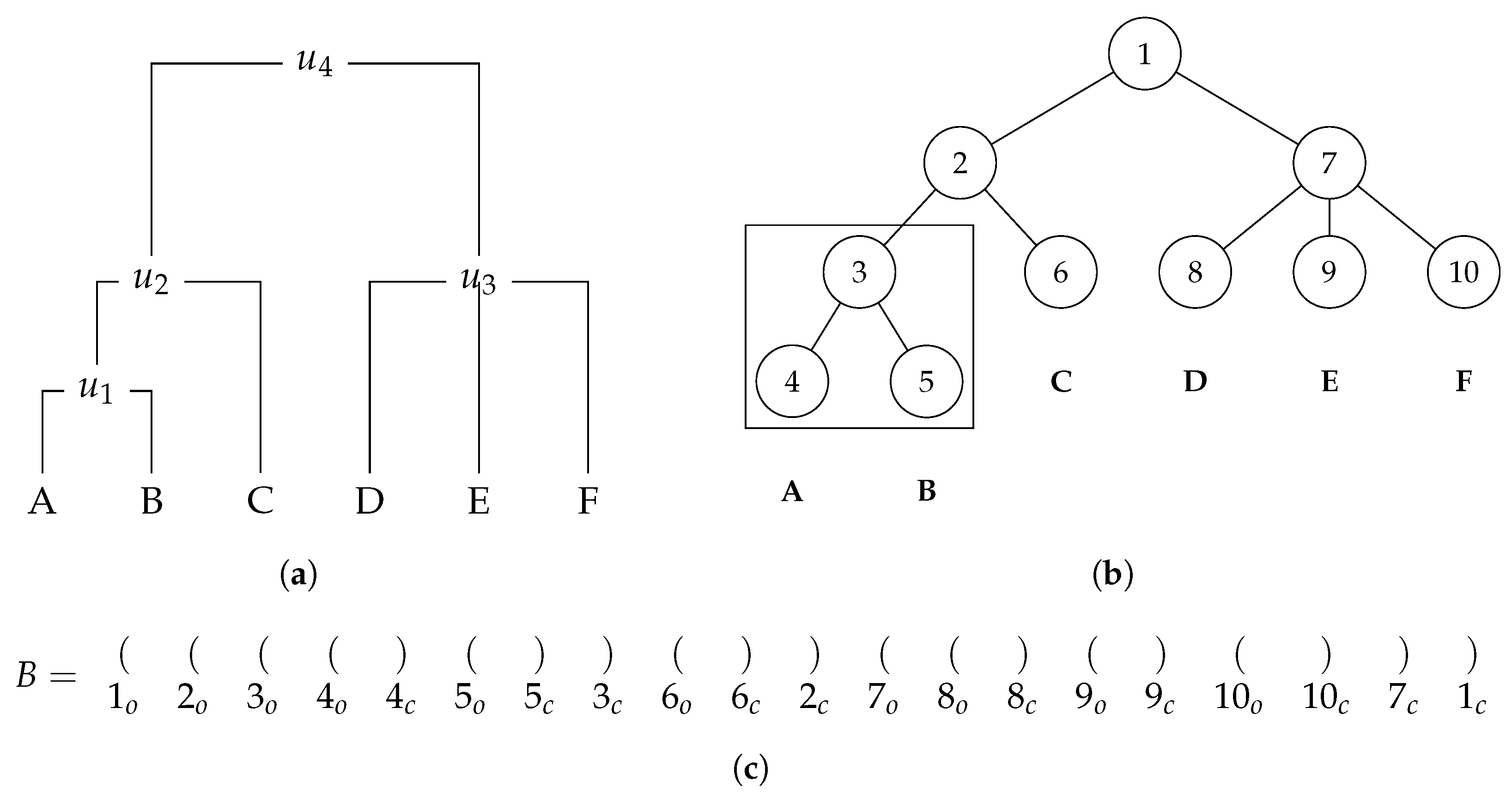
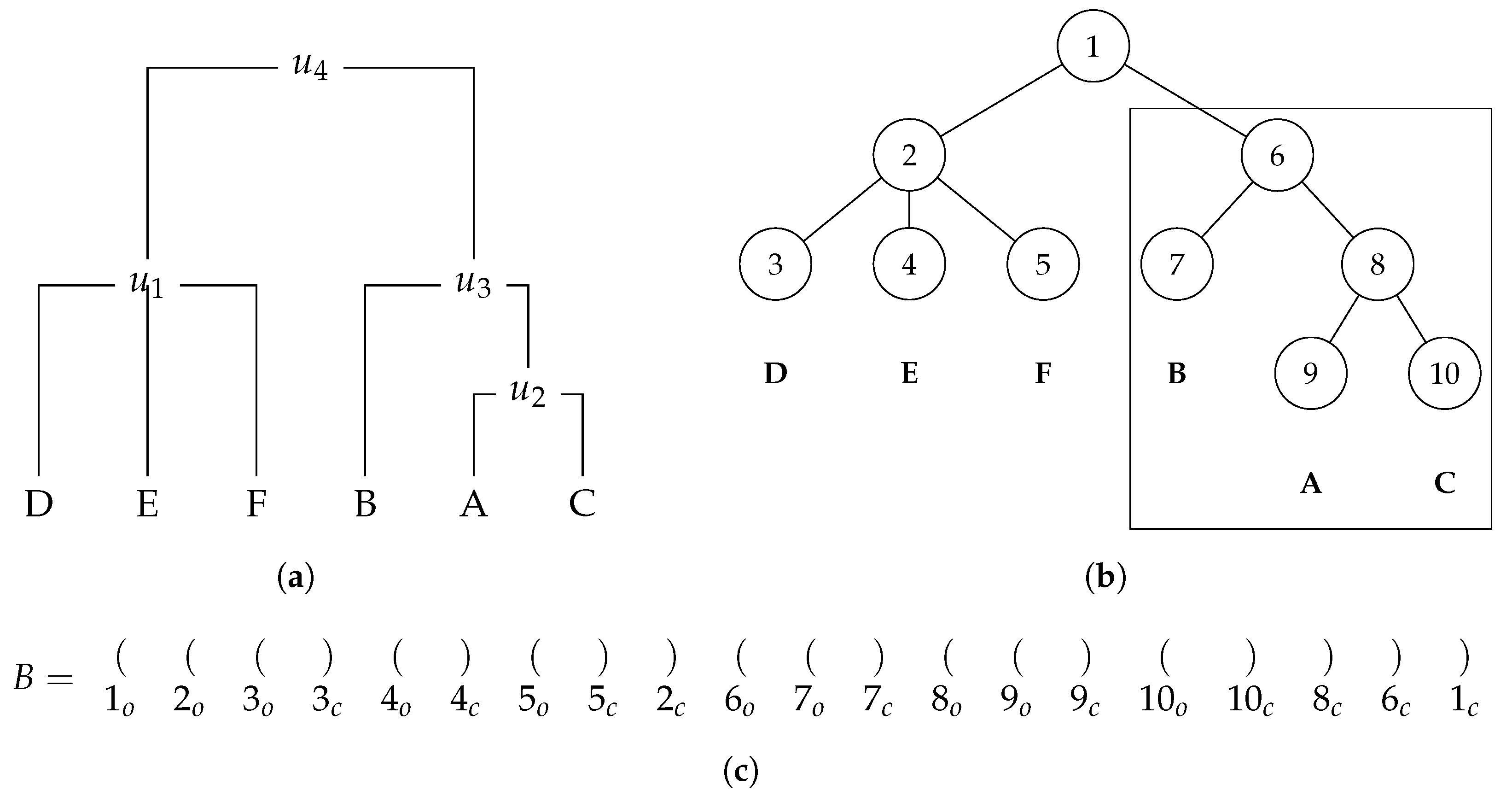
A balanced parentheses representation is a method frequently used to represent hierarchical relationships between nodes in a tree, closely related to the newick format described before. Figure 4 depicts an example of a rooted labelled phylogenetic tree and its balanced parentheses representation. In this kind of representation, there are some key rules to understand how a tree can be represented by a sequence of parentheses. The first rule is that each node is mapped to a unique index given by the tree pre-order transversal. For instance, in Figure 4, a node with label A is mapped to 4. The second rule is that each node is represented by a pair of opening and closing parentheses. For example, in Figure 4, a node with index 4 is represented by the parentheses in 4th and 5th positions. In terms of memory representation, the bit vector keeps this information, where the opening parentheses are represented as a 1 and the closing ones as a 0. This is the reason why the size of the bit vector is 2 times the number of nodes. We notice that it is not necessary to explicitly store the index of each node.

The third rule is that for all nodes present in the tree, all their descendants appear after the opening parentheses and before the closing parentheses that represent them. For example, in Figure 4, the opening and closing parentheses that represent the third node are in Positions 3 and 8, respectively. Then, we can conclude that the parentheses that represent its descendants (Nodes 4 and 5) are in Positions 4, 5, 6, and 7, which are between 3 and 8. Throughout this document, we refer to an index of a node as i and to a position in a bit vector as p.

3.2. Operations

There are several operations that are fundamental to manipulate the bit vectors that encode each tree effectively. The most important ones in the present context are operations Rank1, Rank10, Select1, Select0, FindOpen, FindClose, and Enclose. Then, we added operations PreOrderMap, IsLeaf, LCA, ClusterSize, PreOrderSelect, PostOrderSelect and NumLeaves that mostly use the fundamental operations just mentioned before. In

Table 1. Operations on bit vectors, on balanced sequences of parentheses and on trees (see [23] for details), grouped, respectively. We note that a balanced sequence of parentheses and a tree are represented by bit vector $bv$ given as an argument.

Operation	Meaning	Complexity
Rank1($bv,p$)	Returns the number of occurrences of ‘1’ until position p.	$O\left(1\right)$
Rank10($bv,p$)	Returns the number of occurrences of ‘10’ until position p.	$O\left(1\right)$
Select1($bv,i$)	Returns the position for the ith ‘1’.	$O\left(1\right)$
Select0($bv,i$)	Returns the position for the ith ‘0’.	$O\left(1\right)$
Enclose($bv,p$)	Returns the position where the smaller segment strictly containing p is located, with every two matching parentheses defining a segment.	$O(log(n\left)\right)$
Excess($bv,p$)	Returns the number of opening minus the number of closing parentheses until p.	$O\left(1\right)$
FindOpen($bv,p$)	Given a position p, returns the position of the corresponding opening parenthesis.	$O(log(n\left)\right)$
FindClose($bv,p$)	Given a position p, returns the position of the corresponding closing parenthesis.	$O(log(n\left)\right)$
rmq($bv,l,r$)	Given two positions l and r, returns the position with minimum excess in range $[l..r]$.	$O(log(n\left)\right)$
ClusterSize($bv,p$)	Given the opening position p of a node, returns the size of the cluster with that node as root.	$O(log(n\left)\right)$
FirstChild($bv,p$)	Given the opening position p of a node, returns the position for its first child.	$O\left(1\right)$
IsLeaf($bv,p$)	Given the opening position p of a node, returns True it is a leaf and False otherwise.	$O\left(1\right)$
LCA($bv,l,r$)	Given the opening positions l and r of two nodes, returns the opening position of their lowest common ancestor.	$O(log(n\left)\right)$
NumLeaves($bv,p$)	Given the opening position p of a node, returns the number of leaves that have that node as ancestor.	$O(log(n\left)\right)$
PostOrderSelect($bv,i$)	Given the post-order traversal index i of a node, returns its opening position.	$O(log(n\left)\right)$
PreOrderMap($bv,p$)	Given an opening position p of a node, returns its pre-order traversal index.	$O\left(1\right)$
PreOrderSelect($bv,i$)	Given the pre-order traversal index i of a node, returns its opening position.	$O\left(1\right)$

, it is possible to see the list of operations as well as their meaning and their run time complexity; see the text by Navarro [23] for details on primitive operations. More details in the implementation of the added operations can be found in Appendix A.

3.3. Robinson–Foulds Distance Computation

To compute the Robinson–Foulds distance, our algorithm receives as input two bit vectors that represent the two trees being compared, as well as a mapping between tree indexes. This mapping can be represented by an array of n integers such that the position of each integer corresponds to the index minus one on the first tree, and the integer value at that position in the array corresponds to the index on the second tree. This way, it is possible to obtain the index of the node with a given label in the second tree given the index of where it is in the first tree. We notice that we only maintain the indexes that correspond to have labels, the others remain with a value of zero. An example of this map for the trees in Figure 4 and Figure 5 is

$$\begin{array}{ccccccccccccc}\hfill \mathrm{index}\mathrm{on}{T}_5& [& 0& 0& 0& 9& 7& 10& 0& 3& 4& 5& ]\\ \hfill \mathrm{index}\mathrm{on}{T}_4(-1)& & 0& 1& 2& 3& 4& 5& 6& 7& 8& 9& \end{array}.$$

(1)

As mentioned before, this mapping can be represented in a more compact form. If we take the labels in the trees and enumerate them in some canonical order, assigning them identifiers from 1 to n, then each tree represents a permutation $\pi$ of that enumeration. Hence, given T and the associated permutation $\pi$, $\pi \left[i\right]$ is the label at the node of T with index i, and ${\pi }^{-1}\left[i\right]$ is the index of the node of T with label i, for $i\in \{1,\dots ,n\}$. By composing both permutations, we can determine the bijection among the nodes of both trees. Since each permutation can be represented with $(1+\epsilon )nlogn$ bits, allowing for finding $\pi \left[i\right]$ in constant time and ${\pi }^{-1}\left[i\right]$ in $O(1/\epsilon )$ time [23], we obtain a more compact representation than the previous construction. In what follows, for simplicity, we consider the mapping representation through an array of integers.

Then, the algorithm counts the number of clusters present in both trees. This is achieved by examining the first tree in a post-order traversal and verifying, for all clusters, whether they are present in the second tree. To verify whether a cluster from the first tree is present in the second tree, the key idea is to obtain the cluster from the second tree that is described by the lowest common ancestor (LCA) among all the taxa present in that cluster. Then, if the number of taxa present in the cluster that was obtained is equal, we can guarantee that the cluster is present in both trees. For example, we consider $T_4$ and $T_5$ as the trees represented in Figure 4 and Figure 5, respectively. To verify whether the cluster highlighted in $T_4$, namely $\{A,B\}$, is present in $T_5$, we first need to calculate the index of both taxa A and B. In the balanced parentheses representation of $T_4$, A and B occur in positions 4 and 5, respectively. Then, using the map, we can conclude that in balanced parentheses representation of $T_5$, A and B occur in positions 9 and 7, respectively. Then, by computing the LCA in $T_5$ between those nodes, index 6 is obtained, which represents the cluster highlighted in $T_5$. Given that, this cluster contains three leaves and the original one contains just two, and thus it can be concluded that cluster $A,B$ is not present in $T_5$.

To efficiently compute this distance, the trees are traversed in a post-order traversal. This is performed to guarantee that all nodes are accessed before their ancestors. This way, it is possible to minimize the number of times that the LCA operation is called. For example, considering $T_4$ as the tree represented in Figure 4. As mentioned before, when computing the LCA between nodes A and B, the value of which is 6, we can conclude that the cluster is not present on tree $T_5$. When computed, each LCA value is saved on a stack associated to the node with index 3 of $T_4$.

Continuing the post order, we now obtain for taxa C that its position in $T_4$ is 6 and, consulting the map, its position in $T_5$ is 10. Then, to check whether cluster $A,B,C$ is also present in $T_5$, we use the LCA stored in a node with index 3 of $T_4$, i.e., 6 and Position 10 to compute the new LCA value. The new LCA value is also in Position 6 and is saved on a stack associated to the node with index 2 of $T_4$. Since in this case the cluster obtained in $T_5$ has the same number of leaves as cluster $A,B,C$ in $T_4$, we can conclude, by construction, that it is the same cluster. This process continues until it reaches the tree root. We ntoice that when there are only labels on the leaves, the internal nodes are not included in clusters.

In our approach, we do not count the singleton clusters, since they occur in both trees. Moreover, the internal nodes of each tree offer us the number of non-singleton clusters present on that tree. Then, knowing the number of clusters from both trees and the number of clusters that are present in both trees, we can conclude the number of clusters that are not common to both trees, therefore knowing the Robinson–Foulds distance. In Section 4, we present more details on the implementation of the RF algorithm.

3.4. The Extended/Weighted Robinson–Foulds

Our algorithm can also compute the Robinson–Foulds distance for trees with taxa in internal nodes and/or with weights on edges (eRF, wRF, weRF). For internal labelled nodes, the approach is very similar to the previous one. The only difference is that it is also necessary to compute the LCA for the taxa inside the internal nodes. Then, to determine whether the clusters are the same, instead of comparing the number of leaves, we determine whether the sizes of the clusters are the same. More details on these differences can be found in Appendix B.

Computation of the weighted Robinson–Foulds distance can be perfomed by storing the total sum of the weights of both trees. Then, we verify whether each cluster is present in the second tree; if that is the case, we subtract the weights of the cluster in both trees and add the absolute difference between the two of them. This approach can be seen as first considering that all clusters are present in only one tree and then correcting for the clusters that are found in both trees. More details on these differences can be found in Appendix B.

3.5. Information about the Clusters

When applying the algorithms described above, it is also possible to store the clusters that are detected in both trees. This can be achieved through adding to a vector the indexes of the cluster in the first and second tree when concluding that they are the same. This allows for us to check whether the distance returned by the algorithm is correct and whether the differences between the trees are well represented by the distance computed.

4. Implementation

Our algorithms are implemented in C++ and are available at https://github.com/pedroparedesbranco/TreeDiff (accessed on 20 December 2023). All algorithms are divided into two phases, namely the parsing phase and the distance computation. The first phase of all implemented algorithms receives two trees in a Newick format. Then, the goal is to parse this format, create the two bit vectors that represent both trees and mapping (CodeMap) to correlate the indexes of both trees. The second phase of each algorithm receives as input the two bit vectors and the mapping, and computes the corresponding distance. To represent the bit vectors, we used the Succinct Data Structure Library (SDSL) [30] which contains three implementations to compute the fundamental operations mentioned in Section 3.2. We chose the bp_support_sada.hpp [29] since it was the one that obtained the best results in terms of time and space requirements. The mapping that correlates the taxa between both trees relies on integer keys of 32 bits in our implementation.

4.1. Parsing Phase

In the first phase, when parsing the Newick format, the construction of the bit vectors is straightforward since the newick format already has the parentheses in order to represent a balanced parentheses bit vector. The only detail that we need to take into account is that when we encounter a leaf, we need to add two parentheses, the first one open and the second one closed (see Algorithm 1).

The mapping (CodeMap) exemplified in Equation (1) is also built in the first phase. For this process, we need to have a temporary hash table that associates the labels found in the Newick representation to the indexes of the first tree (HashTable). When a labelled node is found while traversing the first tree, it is added to the HashTable associating the label and the index where it is located in the tree. Then, when a labelled node is found in the second tree, the algorithm looks for that label in the HashTable to find index i where it is located in the first tree. Then, it stores in position $i-1$ of the CodeMap the index where that label is located in the second tree.

To compute the wRF distance, it is also necessary to create two float vectors to save the weights that correspond to a given cluster c for each tree, i.e., $w_T\left(c\right)$ in Definition 3. These weights are stored in the position that corresponds to the index where they are located in each tree. This process can be seen in Algorithm 1. The first phase takes linear time with respect to the number of nodes if we have a weighed or fully labelled tree, otherwise it takes linear time with respect to labelled nodes.

4.2. Distance Calculation

The second phase is the computation of the Robinson–Foulds distance or one of its variants. We extended the functionality of SDSL to support more operations, as previously mentioned. More details are available in Appendix A.

For the RF distance and its variants, two different approaches were implemented that guarantee that the algorithm traverses the tree in a post-order traversal. The first one, which we designated by rf_postorder, takes advantage of the PostOrderSelect operation, while the second one, which we designated by rf_nextsibling, takes advantage of NextSibling and FirstChild operations.

4.2.1. Robinson–Foulds Using PostOrderSelect

To make sure that the tree is traversed in a post-order traversal, this implementation simply performs a loop from 1 to n and calls the function PreOrderSelect for all the values. This implementation also uses a very similar strategy to the one used in the Day algorithm [19] to keep the LCA results computed earlier. This strategy consists in using a stack that keeps track, for each node, of the index of the corresponding cluster from the second tree and the size of the cluster from the first tree. Then, whenever a leaf is found, the corresponding index is added, as well as the size of the leaf, which is one. When the node found is not a leaf, it moves through the stack and finds the last nodes that where added until the sum of their sizes is equal to the size of the cluster. For these nodes, the LCA between each pair is computed while removing them from the stack. When this process is finished, it is possible to verify whether that cluster is present in the other tree and then add the information of that cluster to the stack so that the computations of the LCA that where performed are not performed again. An implementation of this process can be seen in Algorithm 2.

Despite the strategy of using a stack being similar to that of the Day algorithm, our approach just stores in Stack 2 integers for each node, while in the Day algorithm, it is necessary to store 4 integers for each node, namely the value of the left leaf; the value of the right leaf; the number of leaves below; and the size of the cluster. Moreover, with our approach, there is no need to create the cluster table as the Day algorithm need since we use the LCA to verify the clusters.

Given that the algorithm moves through each node in the first tree and needs to compute LCA, PostOrderIndex and number of leaves NumLeaves from each cluster, the theoretical complexity of the algorithm is $O(nlog(n\left)\right)$, with n being the number of nodes in each tree.

Algorithm 1 Parsing Phase

1: Input: $T_1,T_2$ in Newick format.   2: Output: $b{v}_1,b{v}_2,w_1,w_2,CodeMap,weightsSum$  ▹$w_1$, $w_2$ and $weightsSum$ are only used for wRF and weRF distances   3: $HashTable\leftarrow null$   4: $weightsSum\leftarrow 0$   5: for $i=1;i<3;i++$ do   6:       $b{v}_i\leftarrow null$   7:       $index\leftarrow$ 0   8:       $s\leftarrow null$                                      ▹s is a stack of integers   9:       while $c\leftarrow \mathtt{getChar}\left(T_i\right)\ne ;$ do 10:             if $c{=}^{\prime }{(}^{\prime }$ then 11:                   $\mathtt{push}(s,index)$ 12:                   $index$++ 13:                   $\mathtt{push}\_\mathtt{back}(b{v}_i,1)$ 14:             else if $c{=}^{\prime }{,}^{\prime }$ then 15:                   continue 16:             else if $c{=}^{\prime }{)}^{\prime }$ then 17:                   $c\leftarrow \mathtt{getChar}\left(T_i\right)$ 18:                   if not ($c{=}^{\prime }{{)}^{\prime }\mathbf{or} c{=}^{\prime }(}^{\prime }\mathbf{or} c{=}^{\prime }{,}^{\prime }\mathbf{or} c{=}^{\prime }{;}^{\prime }$) then 19:            if $c=:$ then 20:        $c\leftarrow \mathtt{getChar}\left(\right)$ 21:        $weight\leftarrow \mathtt{getWeight}\left(T_i\right)$ 22:        $w_i\left[index\right]\leftarrow weight$ 23:        $weightsSum\leftarrow weightsSum+weight$ 24:            else 25:        $label\leftarrow \mathtt{getLabel}\left(T_i\right)$ 26:        if $i=1$ then 27:           $HashTable\left[label\right]\leftarrow index$ 28:        else 29:           $CodeMap\left[HashTable\right[label\left]\right]\leftarrow count$ 30:        end if 31:            end if 32:                   else 33:            $c\leftarrow \mathtt{ungetChar}\left(T_i\right)$ 34:                   end if 35:                   $\mathtt{pop}\left(s\right)$ 36:                   $\mathtt{push}\_\mathtt{back}(b{v}_i,0)$ 37:             else 38:                   $\mathtt{push}\_\mathtt{back}(b{v}_i,1)$ 39:                   $\mathtt{push}\_\mathtt{back}(b{v}_i,0)$ 40:                   $label\leftarrow \mathtt{getLabel}\left(T_i\right)$ 41:                   if $i=1$ then 42:            $HashTable\left[label\right]\leftarrow index$ 43:                   else 44:            $CodeMap\left[HashTable\right[label\left]\right]\leftarrow count$ 45:                   end if 46:             end if 47:       end while 48: end for 49: $\mathtt{free}\left(HashTable\right)$ 50: Return $b{v}_1,b{v}_2,w_1,w_2,CodeMap,weightsSum$

Algorithm 2 rf_postorder Implementation

1: Input: $b{v}_1,b{v}_2,CodeMap$   2: ▹ Let $numInternalNodes1$ and $numInternalNodes2$ be the number of internal nodes of both trees.   3: Output: Robinson–Foulds distance   4:     5: $equalClusters⟵0$   6: for $i\leftarrow 1$ to N do   7:       $p\leftarrow$PostOrderSelect($b{v}_1,i$)   8:       if IsLeaf($b{v}_1,p$) then   9:          $lca\leftarrow$PreOrderSelect($b{v}_2,CodeMap[$PreOrderMap($b{v}_1,p$) − 1] + 1) 10:          $size\leftarrow 1$ 11:          push($s,\langle lca,size\rangle$)                          ▹ Let s be a stack. 12:       else 13:          $cs\leftarrow$ClusterSize($b{v}_1,p$) 1 14:          while $cs\ne 0$ do 15:             $\langle lca,size\rangle \leftarrow$pop(s) 16:             if $lcas!=null$ then 17:                $\langle lca,size\rangle \leftarrow$pop(s) 18:                $lcas\leftarrow$LCA($b{v}_2,lcas,lca$) 19:             end if 20:             $cs=cs-size$ 21:          end while 22:          if NumLeaves($b{v}_1,p$) = NumLeaves($b{v}_2,lcas$) then 23:             $equalClusters\leftarrow equalClusters$ + 1 24:          end if 25:          push(s,$\langle lcas,$ClusterSize($b{v}_1,p$) + $1\rangle$) 26:          $lcas\leftarrow -1$ 27:       end if 28: end for 29: $distance\leftarrow (numInternalNodes1+numInternalNodes2-2\times equalClusters)/2$ 30: return $distance$

4.2.2. Robinson–Foulds Using NextSibling and FirstChild

This implementation takes a slightly different approach. It uses a recursive function that is called for the first time for the root node. Then, it verifies whether the given node is not a leaf and, if that is the case, it calls the function to the first child node. Then, for all the calls, it examines all the siblings of the given node and computes the LCA between all of them. Whenever the node in question is not a leaf, the algorithm uses the LCA value computed and operation NumLeaves to verify whether the cluster is common to both trees. The function returns the index of LCA obtained so that in this implementation, there is no need to keep an explicit stack to reuse the LCA values computed throughout the algorithm. An implementation of this process can be seen in Algorithm 3.

4.2.3. Weighted/Extended Robinson–Foulds

We also implemented eRF, wRF and weRF distances using PostOrderSelect, and using NextSibling and FirstChild. There are just a few differences with respect to Algorithms 2 and 3. For instance, when phylogenetic trees are fully labelled, it is also necessary to take into account the labels of internal nodes for LCA computation. In the weighted variations, it is also necessary to have two vectors of size n, where n is the number of nodes of each tree, and variable weightsSum, which is updated during the tree transversal. More details can be found in Appendix A, with the implementation of eRF and wRF using PostOrderSelect.

Algorithm 3 rf_nextsibling Implementation

1: Input: $b{v}_1,b{v}_2,CodeMap$   2: ▹ To guarantee a post-order transversal, the initial call to this function initiates current to tree root index   3: ▹ Let $numInternalNodes1$ and $numInternalNodes2$ be the number of internal nodes of both trees.   4: Output: Robinson–Foulds distance   5:     6: $equalClusters⟵0$   7: rf_nextsibling_aux$\left(0\right)$   8: $distance\leftarrow$ ($numInternalNodes1+numInternalNodes2-2\times equalClusters)/2$   9: return $distance$ 10:   11: procedure rf_nextsibling_aux($current$): int 12:       if IsLeaf($b{v}_1,current$) then 13:          $lcas\leftarrow$PreOrderSelect($b{v}_2,CodeMap[$PreOrderMap($b{v}_1,current$) − 1] + 1 14:       else 15:          $lcas\leftarrow$rf_nextsibling(FirstChild($b{v}_1,current$)) 16:          if NumLeaves($b{v}_1,current$) = NumLeaves($b{v}_2,lcas$) then 17:            $equalClusters\leftarrow equalClusters$ + 1 18:          end if 19:       end if 20:       while current ←NextSibling($b{v}_1,current$)!= −1 do 21:          if IsLeaf($b{v}_1,current$) then 22:            $lcas\leftarrow$LCA($b{v}_2$, $lcas$, PreOrderSelect($b{v}_2,CodeMap[$PreOrderMap($b{v}_1,current$) − 1] + 1) 23:          else 24:            lcas_aux ←rf_nextsibling(FirstChild($b{v}_1,current$)) 25:            $lcas\leftarrow$LCA($b{v}_2$, $lcas,lcas\_aux$) 26:            if NumLeaves($b{v}_1,current$) = NumLeaves($b{v}_2,lcas\_aux$) then 27:               $equalClusters\leftarrow equalClusters$ + 1 28:            end if 29:          end if 30:       end while 31:       return $lcas$ 32: end procedure

4.3. Time and Memory Analysis

We also implemented the Day algorithm so that we could compare it with our implementation in terms of running time and memory usage. This algorithm was also implemented in C++. It stores two vectors of integers with size n for each tree and two vectors of integers with size $n/2$ (the number of leaves). The complexity of the algorithm is $O\left(n\right)$ with respect to both time and space.

The complexity of both parsing phases, namely the Day approach and our approach, is $O\left(n\right)$, since they loop through all the nodes. The complexity of the Day algorithm with respect to the RF computation phase is also $O\left(n\right)$. With respect to the second phase of our approach, we depict the complexity analysis with respect to the number of times LCA, NumLeaves, ClusterSize, PostOrderSelect and NextSibling are called and which depends on n.

For RF computed with rf_postorder implementation, the PostOrderSelect operation is called for each node n times. The number of times LCA is called is equivalent to the number of leaves minus the number of first leaves which in the worst case is $n-2$. This case would be a tree that only contains the root as an internal node. With respect to NumLeaves operation, it is called two times for each internal node, with the worst case being $2\times (n-1)$. This case is when a tree only has one leaf. ClusterSize operation is called one time for each internal node, which results in $n-1$ in the worst case as before. In total, the complexity is $(n+(n-2)+(2\times (n-1))+(n-1\left)\right)\times O(log(n\left)\right)=(5n-5)\times O(log(n\left)\right)$. However, the worst case for LCA operations is the best case for NumLeaves and ClusterSize and vice versa. This means that in the worst case, LCA operation is applied 0 times and the complexity is $(4n-3)\times O(log(n\left)\right))$.

For RF computed with rf_nextsibling implementation, the number of calls for LCA and NumLeaves is the same as before. The number of NextSibling operation calls is the same as that of LCA operation. This means that the complexity for this case is $\left(\right(n-2)+(n-2)+(2\times (n-1)\left)\right)\times O(log(n\left)\right)=(4n-5)\times O(log(n\left)\right)$; however, for the same reason as before, it can be reduced to $(2n-2)\times O(log(n\left)\right)$.

For the wRF distance computed by both rf_postorder and rf_nextsibling implementations, the number of times these operations are called is the same as that of the original RF. For eRF and weRF computed by both implementations, the only difference is that the LCA operation is called also for all internal nodes. This means that the number of times the LCA operation is applied is equivalent to the total number of nodes minus the number of first leaves. This changes the complexity in both implementations. In rf_postorder, it changes to $(5n-4)\times O(log(n\left)\right)$ since the number of LCA calls passes from 0 to $n-1$ in the worst case. In rf_nextsibling, it changes to $(3n-3)\times O(log(n\left)\right)$. All implementations referred above have then a running time complexity of $O(nlog(n\left)\right)$.

In terms of memory usage, RF computed by both rf_nextsibling and rf_postorder implementations only uses two bit vectors of size $2n$ and a vector of 32 bit integers with size n, so the total of bits used is $36n$ bits; however, the last one needs an additional stack to save LCA values. And the efficient implementation of primite operations over the bit vectors require extra $o\left(n\right)$ bits. The Day algorithm (rf_day implementation) needs four vectors of 32 bit integers with size n as well as two vectors of 32 bit integers with the size equal to the number of leafs which is equal to $n-1$ in the worst case. This results in $32\times 4n+32\times 2(n-1)=192n-64$ bits.

5. Experimental Evaluation and Discussion

In this section, the performance of rf_postorder and rf_nextsibling implementations is discussed in comparison to their baselines and extensions. To evaluate the implementations, we used the ETE Python library to create a random generator of trees in the Newick format. To evaluate the RF distance, 10 trees (5 pairs) were generated, starting with 10,000 leaves and up to trees with 100,000 leaves, with a step of 10,000. Not only five pairs of trees were denerated with information only on the leaves for all the sizes tested, but also fully labelled trees. We also considered in our evaluation the phylogenetic trees inferred from a real dataset from EnteroBase [22], namely Salmonella core-genome MLST (cgMLST) data, with 391,208 strains and 3003 loci. To analyze the memory usage, the valgrind massif tool [31] was used.

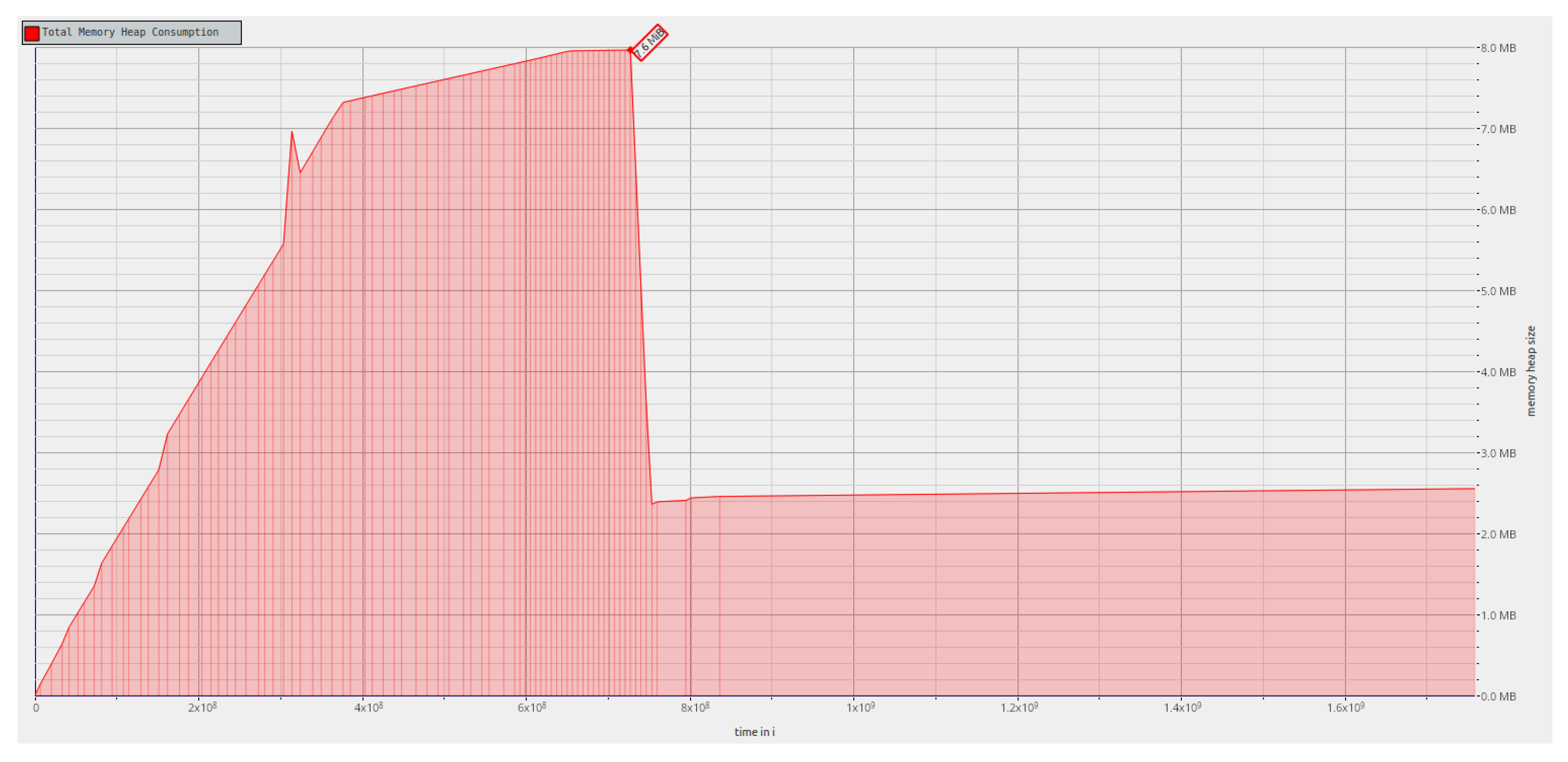
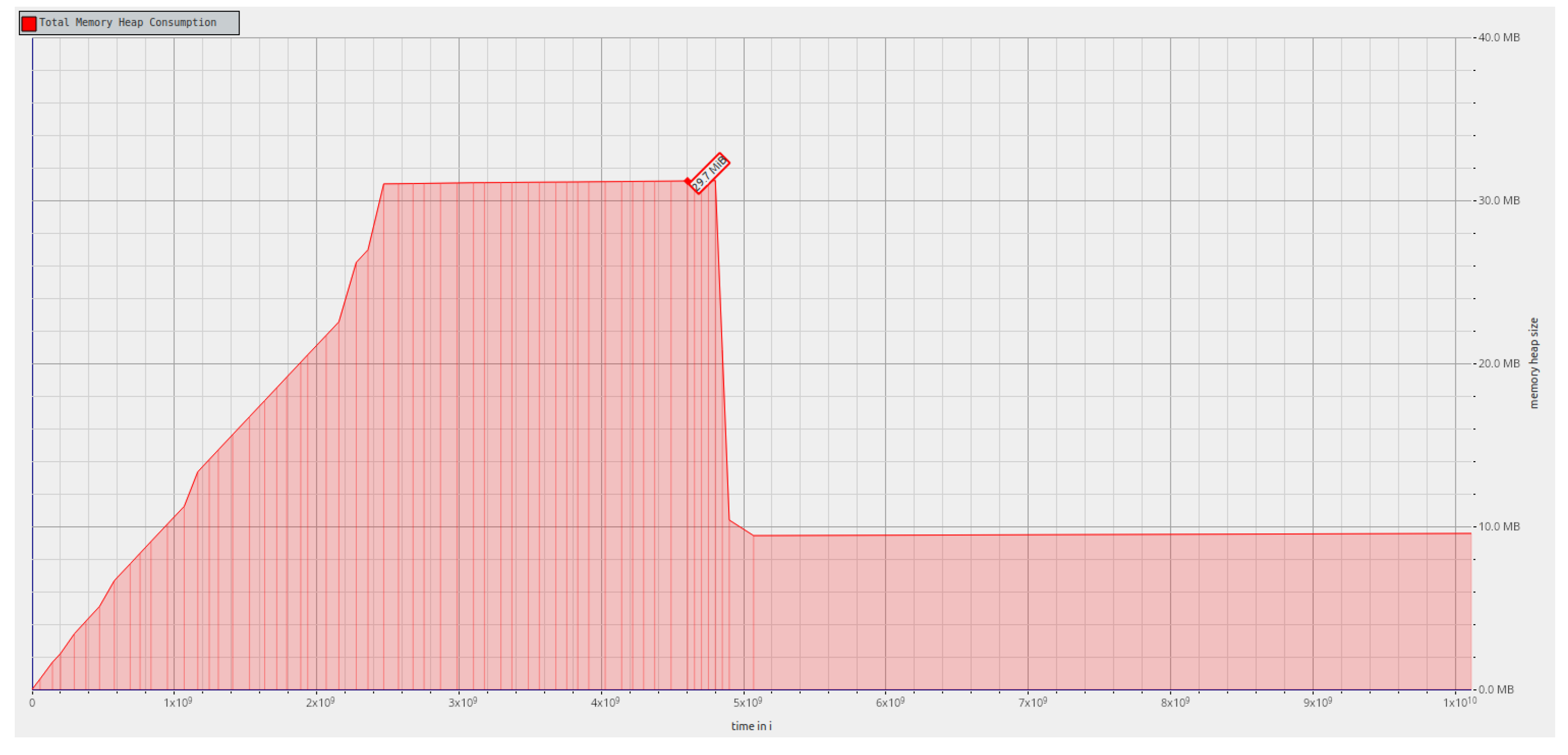
First, the memory used throughout the rf_postorder algorithm execution was analyzed for a tree that with 100,000 leaves. Figure 6 shows that for the first phase, the memory consumption is higher since a hash table has to be used to create the map that correlates labels and tree indexes. In the transition to the second phase, since the hash table is no longer needed and, as such, the memory it required is freed, the memory consumption falls abruptly. In the second phase of the algorithm, the memory consumption is lower since this phase only uses the information stored in the two bit vectors and related data structures, and in the mapping that correlates the two trees. We note that by serializing and storing the trees and related permutations as their bit vector representations, we can avoid the memory required for parsing the Newick format.

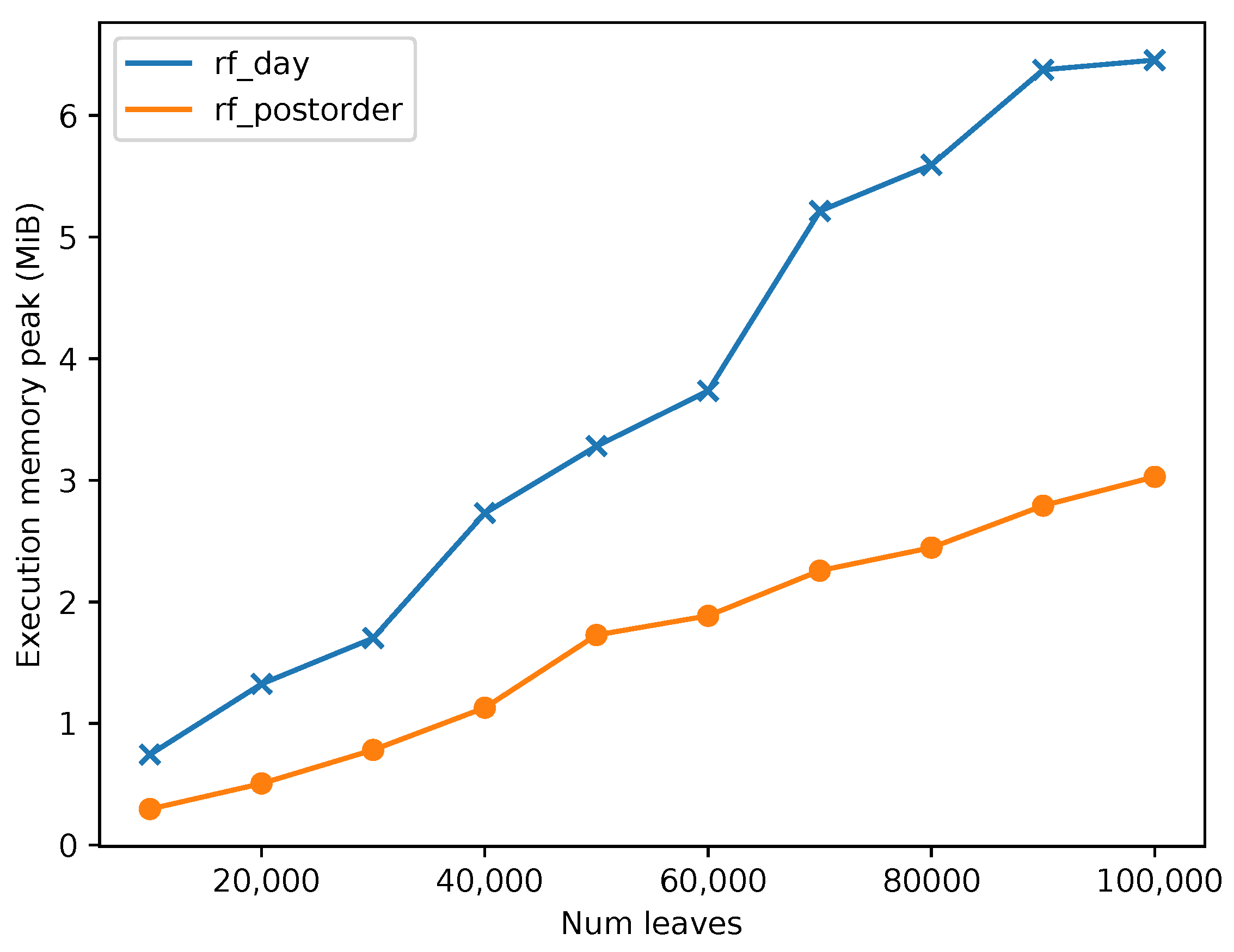
Second, the memory usage for the second phase of rf_postorder and rf_day implementations was compared. Figure 7 shows the comparison between the two algorithms in terms of their memory peak usage. rf_postorder exhibits a significant lower memory peak compared to the rf_day algorithm. We note that the difference is smaller than expected in our theoretical analysis since in our implementations we are keeping track of common clusters, as described in Section 3.5, and extra space is required for supporting fast primitive operations over the bit vectors. If we omit that cluster tracking mechanism, we can reduce further the memory usage of our implementations.

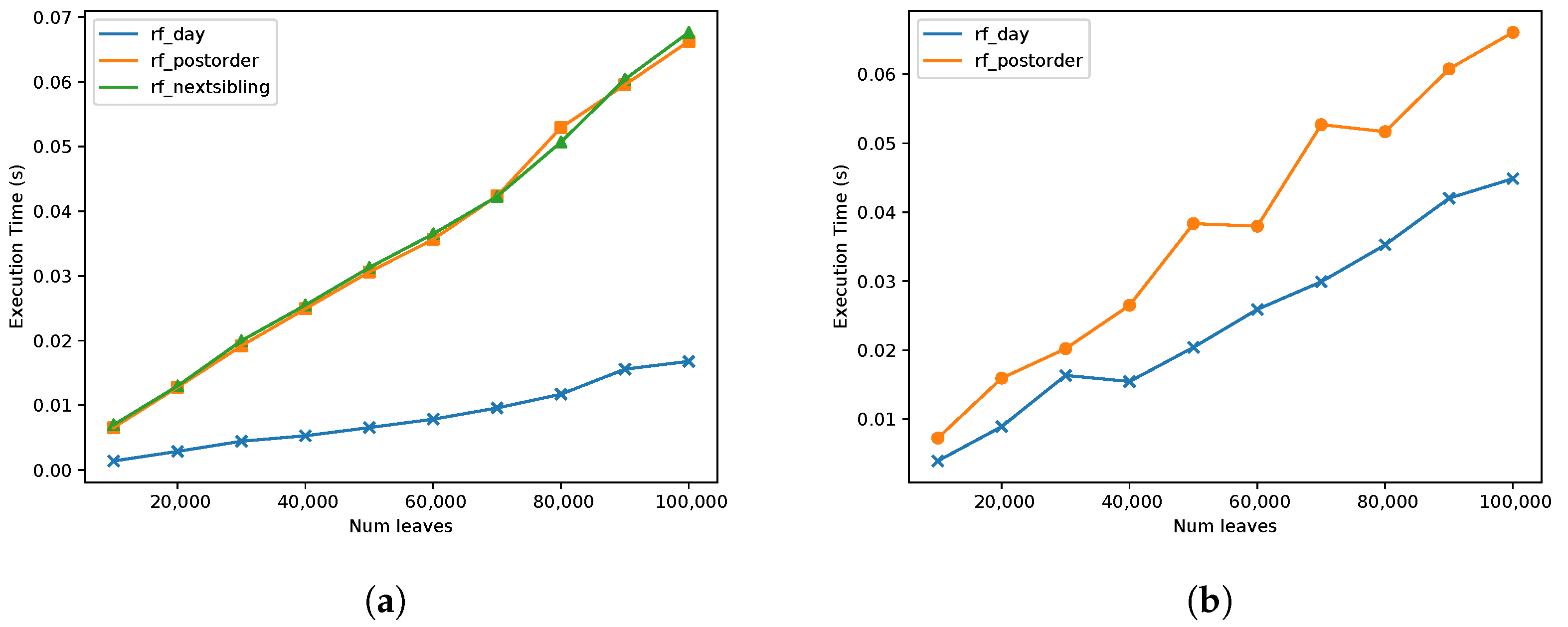
Then, the running time between the two algorithms was compared for the parse and algorithm phases; Figure 8. For the parse phase, we only compared rf_postorder with rf_day since rf_nextsibling has the exact same parsing phase as rf_postorder. It can be observed in Figure 8b that the differences between the running time of the two implementations are not significant, indicating similar performances between the two algorithms. In the second phase, a comparison was made between all three implementations. In Figure 8a, it can be observed that both rf_postorder and rf_nextsibling implementations presented almost the same results. Even though the theoretical complexity of those implementations is $O(nlog(n\left)\right)$, in practice, it seems to be almost linear. This finding suggests that the operations used to traverse the tree tend to be almost $O\left(1\right)$ in practice even though they have a theoretical complexity of $O(log(n\left)\right)$. The difference in the running time between these implementation and that of the rf_day one can be explained by the number of operations that are computed for each node as explained previously, and because we used succinct tree representations.

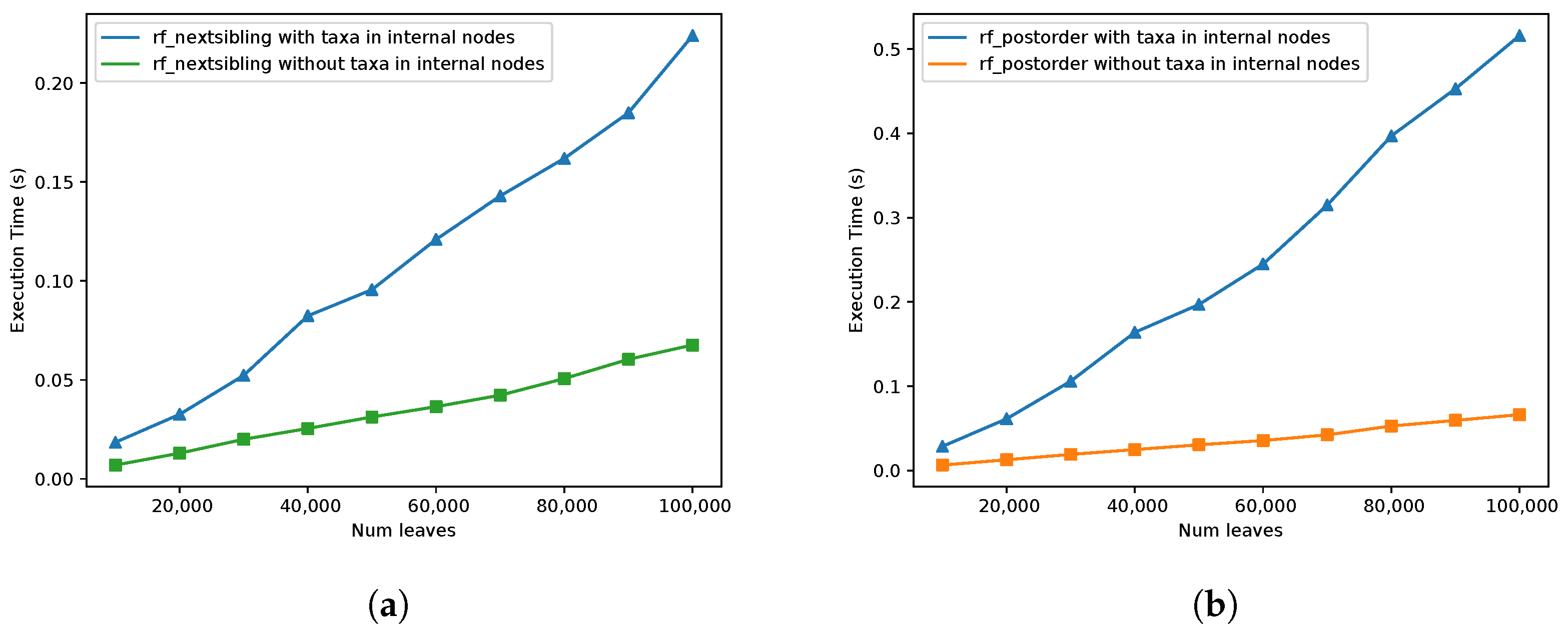
Next, the running time for RF and eRF distances was compared; Figure 9. We note that the Day algorithm does not support fully labelled trees. In both of the rf_postorder and rf_nextsibling implementations, the eRF distance seems to be also linear in practice. However, for the rf_nextsibling implementation, the running time difference seems to be much more insignificant than the difference observed for the rf_postorder implementation. These results are consistent with the theoretical analysis since in rf_nextsibling implementation, the number of times each operation is applied in the worst case is $(3n-3)$ and in the rf_postorder case it is $(5n-4)$. This concludes that the rf_nextsibling implementation provides better results for most trees when it is used to compute the distance for fully labelled trees.

Let us consider now the trees obtained for real data, namely for Salmonella cgMLST data from EnteroBase [22], with 391,208 strains and 3003 loci. We used two pairs of trees obtained for all strains by varying the number of loci being analyzed. Trees were generated using a custom highly parallelized version of the MSTree V2 algorithm [28]. One pair was fully labelled with 391,208 nodes in each tree, and the other pair was leaf labelled with 391,208 leaves. Both pairs represented the same data, they differed only in how data and inferred patterns were interpreted as trees.

Figure 6 shows the memory allocation profile for rf_nextsibling implementation, which is similar for rf_postorder implementation, and for synthetic data. As observed in our previous analysis, for the first phase, the memory consumption is higher due to input parsing. In the second phase, the memory required for parsing is freed, and the memory consumption falls abruptly; in this phase, we have only the information stored in the two bit vectors and related data structures, and in the mapping that correlates the two trees. As discussed earlier, serializing and storing the trees and related permutations as their bit vector representations allow for us to avoid the memory excess required for parsing the Newick format.

Table 2. Run time for Salmonella cgMLST trees, with 391,208 strains.

Algorithm	Implementation	Time (s)	Memory Peak (MiB)
RF using the Day algorithm	rf_day	0.049	25.731
RF using PostOrderSelect	rf_postorder	0.332	9.589
RF using NextSibling and FirstChild	rf_nextsibling	0.319	9.567
wRF using PostOrderSelect	rf_postorder	0.356	18.362
wRF using NextSibling and FirstChild	rf_nextsibling	0.340	18.339
weRF using PostOrderSelect	rf_postorder	0.192	11.668
weRf using NextSibling and FirstChild	rf_nextsibling	0.185	11.658

presents the running time and memory usage for Salmonella cgMLST trees. Figure 10 shows the memory allocation profile for rf_nextsibling implementation. We note that the Day algorithm supports only leaf labelled and unweighted trees; hence, we can only compare it for simple RF. Results for rf_postorder and rf_nextsibling are similar to those observed in synthetic data, with an almost linear increase with respect to both running time and memory usage. We observe that the number of tree nodes for RF and wRF tests is twice as much as those for weRF (a binary tree with 391,208 leaves has 782,415 the nodes in total). And that is reflected in running time and memory usage.

As expected, for both synthetic and real data, both rf_nextsibling and rf_postorder implementations are slower than the Day algorithm implementation, because we have the overhead of using a succinct representation for trees. But it is noteworthy that those implementations offer a significant advantage in terms of memory usage, namely when trees are succinctly serialized and stored. This trade-off between memory usage and running time is common in this setting, with succinct data structures being of practical interest when dealing with large data.

6. Conclusions

We provided implementations of the Robinson–Foulds distance over trees represented succinctly, as well as its extension to fully labelled and weighted trees. These kinds of implementations are becoming useful as pathogen databases increase in size to hundreds of thousands of strains, as is the case of EnteroBase [22]. Phylogenetic studies of these datasets imply then the comparison of very large phylogenetic trees.

Our implementations run theoretically in $O(nlogn)$ time and require $O\left(n\right)$ space. Our experimental results show that in practice, our implementations run in almost linear time, and that they require much less space than a careful implementation of the Day algorithm. The use of succinct data structures introduces a slowdown in the running time, but that is an expected trade-off; we gain in our ability to process much larger trees using space efficiently.

Each tree with n nodes can be represented in $2n+o\left(n\right)+(1+\epsilon )nlogn$ bits, storing its balanced parentheses representation and its corresponding permutation through bit vectors. Our implementations rely on and extend SDSL [30], making use of provided bit vector representations and primitive operations. In our implementations, we did not explore, however, the compact representation of the permutation associated to each tree. Hence, the space used by our implementations can be further improved, in particular if we rely on that compact representation to store phylogenetic trees on secondary storage. We leave this as future work, noting that techniques to represent compressible permutations may be exploited in this setting, leading to a more compact representation [23]; phylogenetic trees tend to be locally conserved and, hence, that favors the occurrence of fewer and larger runs in tree permutations.