Learning to Extrapolate Using Continued Fractions: Predicting the Critical Temperature of Superconductor Materials

Abstract

In the field of Artificial Intelligence (AI) and Machine Learning (ML), a common objective is the approximation of unknown target functions $y=f\left(\mathbf{x}\right)$ using limited instances $S=({\mathbf{x}}^{\left(\mathbf{i}\right)},y^{\left(i\right)})$, where ${\mathbf{x}}^{\left(\mathbf{i}\right)}\in D$ and D represents the domain of interest. We refer to S as the training set and aim to identify a low-complexity mathematical model that can effectively approximate this target function for new instances $\mathbf{x}$. Consequently, the model’s generalization ability is evaluated on a separate set $T=\left\{{\mathbf{x}}^{\left(\mathbf{j}\right)}\right\}\subset D$, where $T\ne S$, frequently with $T\cap S=\varnothing$, to assess its performance beyond the training set. However, certain applications require accurate approximation not only within the original domain D but in an extended domain $D^{\prime }$ that encompasses D as well. This becomes particularly relevant in scenarios involving the design of new structures, where minimizing errors in approximations is crucial. For example, when developing new materials through data-driven approaches, the AI/ML system can provide valuable insights to guide the design process by serving as a surrogate function. Consequently, the learned model can be employed to facilitate the design of new laboratory experiments. In this paper, we propose a method for multivariate regression based on iterative fitting of a continued fraction, incorporating additive spline models. We compare the performance of our method with established techniques, including AdaBoost, Kernel Ridge, Linear Regression, Lasso Lars, Linear Support Vector Regression, Multi-Layer Perceptrons, Random Forest, Stochastic Gradient Descent, and XGBoost. To evaluate these methods, we focus on an important problem in the field, namely, predicting the critical temperature of superconductors based on their physical–chemical characteristics.

1. Introduction

Superconductors are remarkable materials that exhibit the extraordinary property of conducting electrical current with zero resistance. This unique characteristic has led to a wide range of applications. As an example, Magnetic Resonance Imaging (MRI) systems are used globally as a crucial medical tool for producing detailed images of internal organs and tissues. In the face of increasing energy demands driven by renewable energy sources and innovations such as solar cars, superconductors hold great potential for efficient energy transfer.

The elimination of electrical resistance in superconductors significantly reduces energy wastage during current transmission from one location to another. However, a major limitation of existing superconductors is their reliance on extremely low temperatures, known as critical temperatures ($T_c$), to achieve zero resistance. Conventional superconductors described by the Bardeen–Cooper–Schrieffer (BCS) theory (the first microscopic theory of superconductivity since Heike Kamerlingh Onnes’s 1911 discovery of the phenomenon) [1,2] typically exhibit transition temperatures of several Kelvins (i.e., approximately −270 K) [3]. Recently discovered iron-based bulk superconductors demonstrate a highest critical temperature of approximately 56 Kelvin (i.e., at approximately −217 degrees Celsius) [4]. However, these materials are far from being considered high-temperature superconductors (HTS), which are defined as materials that behave as superconductors at temperatures above 77 K (−196.2 degrees Celsius), corresponding to the boiling point of liquid nitrogen. Cuprate superconductors, which are copper oxides combined with other metals, especially rare earth barium copper oxides such as yttrium barium copper oxide, constitute the main class of HTS. The highest critical temperature achieved by cuprates is around 138 K at ambient pressure and possibly 164 K under high pressure. Only cuprate superconductors  [5] and some possible organic superconductors [6] show critical temperature values near or above the liquid nitrogen boiling temperature of −196.2 degrees Celsius. The discovery of HTS has opened up new possibilities for applications that require coolants with low cost and that are easy to handle as well as higher magnetic fields and currents. Therefore, predicting the critical temperature ($T_c$) of superconductors has become a topic of great interest in the field of materials science [7].

In this study, we leverage various machine learning techniques and propose a novel approach based on multivariate continued fractions to develop mathematical models capable of predicting the critical temperature of superconductors. Our models rely solely on the characterization of the chemical structure of the superconducting material by uncovering hidden information within. Accurate prediction of $T_c$ for superconductors can greatly enhance our ability to harness the potential of superconductivity, ushering in a new era of possibilities in multiple fields.

Continued Fraction Regression

In 2019, a new approach for multivariate regression using continued fractions was introduced in [8] and compared with a state-of-the-art genetic programming method for regression. We named this approach ‘Continued Fraction Regression’, or CFR. The best existing algorithm currently utilizes a memetic algorithm for optimizing the coefficients of a model that approximates a target function as the convergent of a continued fraction [8,9]. Memetic Algorithms are well-established research areas in the field of Evolutionary Computation, and the IEEE had established a Task Force in Computational Intelligence for their study. Therefore, it is important to refer readers to a number of the latest references and reviews on the field [10,11]. Very recently, continued fraction regression has been used to obtain analytical approximations of the minimum electrostatic energy configuration of an electron n when the charge is constrained to be on the surface sphere, i.e., the celebrated Thomson Problem. For other applications of continued fraction regression, please see [12] and references therein.

A basic introduction on analytic continued fraction approximation is necessary here. A continued fraction for a real value $\alpha$ has the following form (1) and may be finite or infinite [13] according to whether or not $\alpha$ is a rational number:

$$\alpha =a_0+\frac{b_1}{a_1+\frac{b_2}{a_2+\dots }}$$

(1)

Euler proved a mathematical formula that allows us to write a sum of products as a continued fraction (2):

$$\begin{array}{cc}\hfill \beta =a_0+a_0{a}_1+a_0{a}_1{a}_2+\dots +a_0{a}_1{a}_2\dots a_n& \\ & =\frac{a_0}{1-\frac{a_1}{1+a_1-\frac{a_2}{1+a_2-\frac{\ddots }{\ddots \frac{a_{n-1}}{1+a_{n-1}-\frac{a_n}{1+a_n}}}}}}.\hfill \end{array}$$

(2)

This simple yet powerful equation reveals how infinite series can be written as infinite continued fractions, meaning that continued fractions can be a good general technique to approximate analytic functions thanks to the improved optimization methods such as those provided by memetic algorithms [9]. Indeed, CFR has already demonstrated its effectiveness as a regression technique on the real-world datasets provided by the Penn Machine Learning Benchmarks [9].

In this paper, we use Carl Friedrich Gauss’ mathematical notation for generalized continued fractions [14] (i.e., a compact notation in which “K” stands for the German word “Kettenbruch”, which means ‘Continued Fraction’). Using this notation, we may write the continued fraction in (1) as

$$\alpha =a_0+\underset{i=1}{\overset{\infty }{\mathrm{K}}}\frac{b_i}{a_i};$$

(3)

thus, the problem of finding an approximation of an unknown target function of n variables $\mathbf{x}$ given a training dataset of m samples $S=\left\{({\mathbf{x}}^{\left(\mathbf{i}\right)},y^{\left(i\right)})\right\}$ is that of finding the set of functions $F=\{a_0\left(x\right)...,b_1\left(x\right),...\}$ such that a certain objective function is minimized, i.e., we aim to find

$$f\left(\mathbf{x}\right)=a_0\left(\mathbf{x}\right)+\underset{i=1}{\overset{\infty }{\mathrm{K}}}\frac{b_i\left(\mathbf{x}\right)}{a_i\left(\mathbf{x}\right)}.$$

(4)

2. Materials and Methods

2.1. A New Approach: Continued Fractions with Splines

In previous contributions [8,9], a memetic algorithm was employed to find the approximations. Here, we present another method to fit continued fraction representations by iteratively fitting splines.

Splines provide a regression technique that involves fitting piecewise polynomial functions to the given data [15]. The domain is partitioned into intervals at locations known as “knots”. Then, a polynomial model of degree n is separately fitted for each interval while generally enforcing boundary conditions, including the continuity of the function and continuity of the first $(n-1)$-order derivatives at each of the knots. Splines can be represented as a linear combination of basis functions, of which the standard is the B-spline basis. Thus, fitting a spline model is equivalent to fitting a linear model of basis functions. We refer to Hastie et al. [16] for the particular definition of the B-spline basis.

First, when all the functions $b_i\left(\mathbf{x}\right)=1$, we have a simple continued fraction representation for all i, which we can write as

$$f\left(\mathbf{x}\right)=g_0\left(\mathbf{x}\right)+\frac{1}{g_1\left(\mathbf{x}\right)+\frac{1}{g_2\left(\mathbf{x}\right)+\frac{1}{g_3\left(\mathbf{x}\right)+\dots }}}.$$

(5)

Note that for a term $g_i\left(\mathbf{x}\right)$ we say that it is at a “depth” of i.

Finding the best values for the coefficients in the set of functions $\left\{g_i\left(\mathbf{x}\right)\right\}$ can be addressed as a nonlinear optimization problem as in [8,9]. However, despite the great performance of that approach we aim to introduce a faster variant that can scale well to larger datasets such as this one.

Towards that end, and thinking about the scalability, we fit the model iteratively by depth as follows: we first consider only the first term $g_0\left(\mathbf{x}\right)$ at depth 0, ignoring all other terms. We fit a model for the first term using the predictors $\mathbf{x}$ and target $f\left(x\right)$. Next, we consider only the first and second depths, with the terms $g_0\left(\mathbf{x}\right)$ and $g_1\left(\mathbf{x}\right)$, ignoring the rest. We then fit $g_1\left(\mathbf{x}\right)$ using the previously fit model for $g_0\left(\mathbf{x}\right)$. For example, truncating the expansion at depth 1, we have

$$g_1\left(\mathbf{x}\right)=\frac{1}{f\left(\mathbf{x}\right)-g_0\left(\mathbf{x}\right)}.$$

(6)

Thus, we fit $g_1\left(\mathbf{x}\right)$ using the predictors $\mathbf{x}$ and the target ${(f\left(\mathbf{x}\right)-g_0\left(\mathbf{x}\right))}^{-1}$. We label this target as $y^{\left(1\right)}$. We repeat this process, fitting a new model by truncating at the next depth by using the models fit from previous depths and iterations.

We have that at depth $i>0$, the target $y^{\left(i\right)}$ for the model $g_i\left(\mathbf{x}\right)$ is ${\left({ϵ}_{i-1}\right)}^{-1}\left(\mathbf{x}\right)$, where ${ϵ}_{i-1}\left(\mathbf{x}\right)$ is the residual of the previous depth’s model, $y^{(i-1)}-g_{i-1}\left(\mathbf{x}\right)$.

One notable characteristic of this approach is that if any model $g_i\left(\mathbf{x}\right)$, $i>0$ evaluates to 0, then we will have a pole in the continued fraction, which is often spurious. To remedy this, we modify the structure of the fraction such that each fitted $g_i\left(\mathbf{x}\right)$, $i>0$ is encouraged to be strictly positive on the domain of the training data. To do this, we add a constant $C_i$ to ${ϵ}_i$ when calculating the target $y^{(i+1)}$, where $C_i=\left|{min}_x{ϵ}_i\right|$. Thus, the targets $y^{\left(i\right)}$ for $i>0$ are all non-negative, encouraging each $g_i\left(\mathbf{x}\right)$, $i>0$, to be strictly positive. For example, for $g_1\left(\mathbf{x}\right)$, we would have that the target $y^{\left(1\right)}={(f\left(\mathbf{x}\right)-g_0\left(\mathbf{x}\right)+C_1)}^{-1}$. Of course, we must then subtract $C_i$ from $g_{i-1}\left(\mathbf{x}\right)$ in the final continued fraction model.

We have found that data normalization often results in a better fit using this approach. It is sufficient to simply divide the targets uniformly by a constant when training and multiply by the same constant for prediction. We denote this constant parameter $\mathtt{norm}$.

A good choice of the regression model for each $g_i\left(\mathbf{x}\right)$ is a spline since they are well-established. For reasons stated in the next section, the exception is the first term $g_0\left(\mathbf{x}\right)$, which is a linear model. We use an additive model to work with multivariate data where each term is a spline along a dimension. That is, given m predictor variables, we have that

$$g_i\left(\mathbf{x}\right)=\sum _{j=1}^m{f}_j\left(x_j\right)$$

(7)

for each term $g_i\left(\mathbf{x}\right)$, $i>0$, where each function $f_j$ is a cubic spline along variable j, that is, $f_j$ is a piecewise polynomial of degree 3 and is a function of variable j.

We implement the splines with a penalized cubic B-spline basis, that is, $f_j\left(\mathbf{x}\right)={\sum }_{i=1}^k{\beta }_k{B}_k\left(x_j\right)$, where each $B_i\left(x\right)$ is one of k cubic B-spline basis functions along dimension j and corresponds to one of k knots. We use the following loss function $L\left(\mathbf{B}\left(\mathbf{x},\mathbf{y},\mathit{\beta }\right)\right)$, i.e.,

$$L\left(\mathbf{B}\left(\mathbf{x},\mathbf{y},\mathit{\beta }\right)\right)={\parallel \mathbf{y}-\mathbf{B}\mathit{\beta }\parallel }^2+\lambda \sum _{j=0}^m{\mathit{\beta }}^T{\mathbf{P}}_{\mathbf{j}}\mathit{\beta }$$

(8)

where $\mathbf{B}$ is the matrix of cubic B-spline basis functions for all variables, $\mathit{\beta }$ is the vector of all of the weights, and ${\mathbf{P}}_{\mathbf{j}}$ is the associated second derivative smoothing penalty matrix for the basis for the spline $f_j$. This is standard for spline models [16]. The pseudocode for this approach is shown in Algorithm 1.

Algorithm 1: Iterative CFR using additive spline models with adaptive knot selection

2.2. Adaptive Knot Selection

The iterative method of fitting continued fractions allows for an adaptive method of selecting knot placements for the additive spline models. For the spline model $g_i\left(\mathbf{x}\right)$ at depth $i>0$, we use all of the knots of the spline model $g_{i-1}\left(\mathbf{x}\right)$ at depth $i-1$. Then, for each variable, we place k new knots at the unique locations of the k samples with the highest absolute error from the model $g_{i-1}\left(\mathbf{x}\right)$ at depth $i-1$. As the points with the highest error are likely to be very close to each other, we impose the condition that we take the samples with the highest error, but they must have alternating signs.

In this way, we select k knots for $g_i\left(\mathbf{x}\right)$ and $i>0$, with the first knot at the location of the sample with the highest absolute error computed from the model $g_{i-1}\left(\mathbf{x}\right)$. For the rest of the knots, the $j\mathrm{th}$ knot is selected at the sample’s location with the next highest absolute error after the sample used for the $(j-1)\mathrm{th}$ knot, and only if the sign of the (non-absolute) error of that sample is different from the sign of the (non-absolute) error of the sample used for the $(j-1)\mathrm{th}$ knot. Otherwise, we move on to the next highest absolute error sample, and so on, until we fulfill this condition. This knot selection procedure is shown in Algorithm 2. Note that we let $g_0$ be a linear model, as there is no previous model from which to obtain the knot locations.

Algorithm 2: SelectKnots (Adaptive Knot Selection)

    The goal of using additive spline models with the continued fraction is to take advantage of the continued fraction representation’s demonstrated ability to approximate general functions (see the discussion on the relationship with Padé approximants in [9]). The fraction’s hierarchical structure allows for the automatic introduction of variable interactions, which is not included individually in the additive models that constitute the fraction. The iterative approach to fitting makes for a better knot selection algorithm.

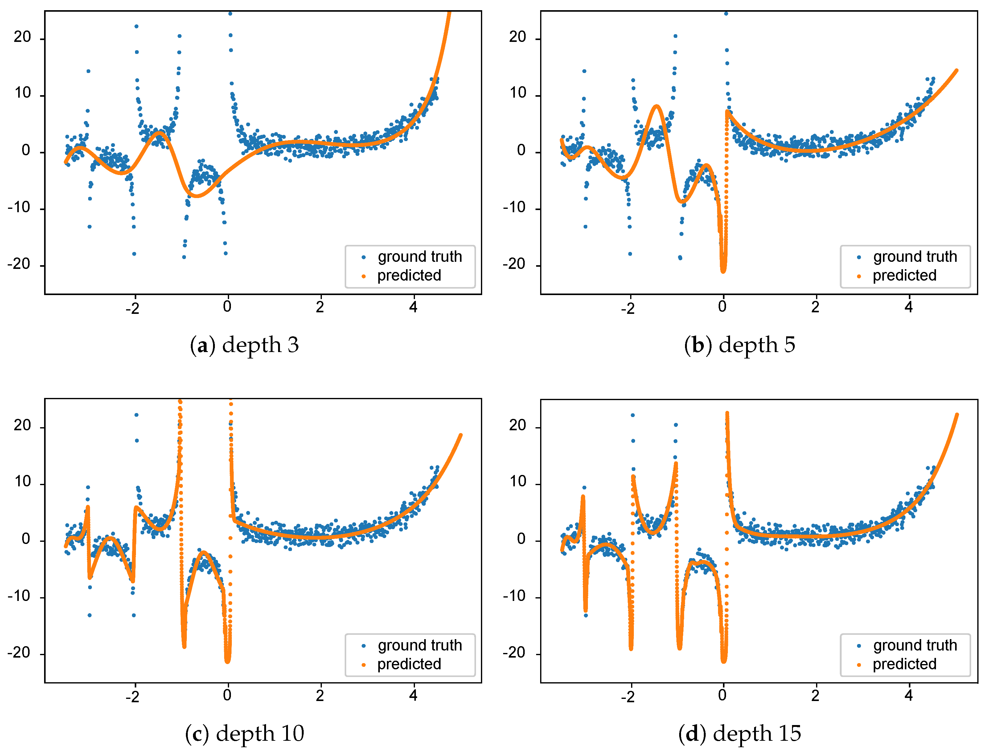
An example of this algorithm modeling the well-known gamma function (with standard normally distributed noise added) is demonstrated in Figure 1. Here, we show how the fitting to gamma is affected by different values of depths (3, 5, 10, 15) in the Spline Continued Fraction. As desired, it is evident from the figure that the Spline Continued Fraction with more depth has a better fit with the data.

2.3. Data and Methods Used in the Study

We used the superconductivity dataset from Hamidieh [7], available from the UCI Machine Learning repository (https://archive.ics.uci.edu/ml/datasets/Superconductivty+Data, accessed on 11 September 2020). The website contains two files. In this work, we only used the train.csv file, which contains information on 21,263 superconductors, including the critical temperature and a total of 81 attributes for each of them.

This dataset on superconductors utilizes elemental properties to predict the critical temperature ($T_c$). The data extraction process involves obtaining ten features from the chemical formula for each of the eight variables, which include Atomic Mass, First Ionization Energy, Atomic Radius, Density, Electron Affinity, Fusion Heat, Thermal Conductivity, and Valence. This results in a total of 80 features. Additionally, the dataset includes one extra feature representing the count of elements present in the superconductor. The dataset encompasses both “oxides” and “metallic” materials, but excludes elements with atomic numbers greater than 86. After performing thorough data preparation and cleaning steps, the final dataset consisted of 21,263 samples, each described by 81 features.

Regarding the elemental distributions of the superconductors in the dataset, Oxygen constitutes approximately 56% of the total composition. Following Oxygen, the next most abundant elements are Copper, Barium, Strontium, and Calcium. As many of the research group’s primary interest is in iron-based superconductors, the following information is likely to be of significant interest to them. Within this dataset, Iron is present in about 11% of the superconductors, with a mean critical temperature ($T_c$) of 26.9 ± 21.4 K. On the other hand, the mean $T_c$ for non-iron-containing superconductors is 35.4 ± 35.4 K. Looking at the overall distribution of $T_c$ values, it is found to be right-skewed, with a noticeable peak centered around 80 K.

For a more detailed understanding of the data generation, feature extraction process, and specific characteristics of the dataset, readers can refer to Hamidieh’s original contribution in [7].

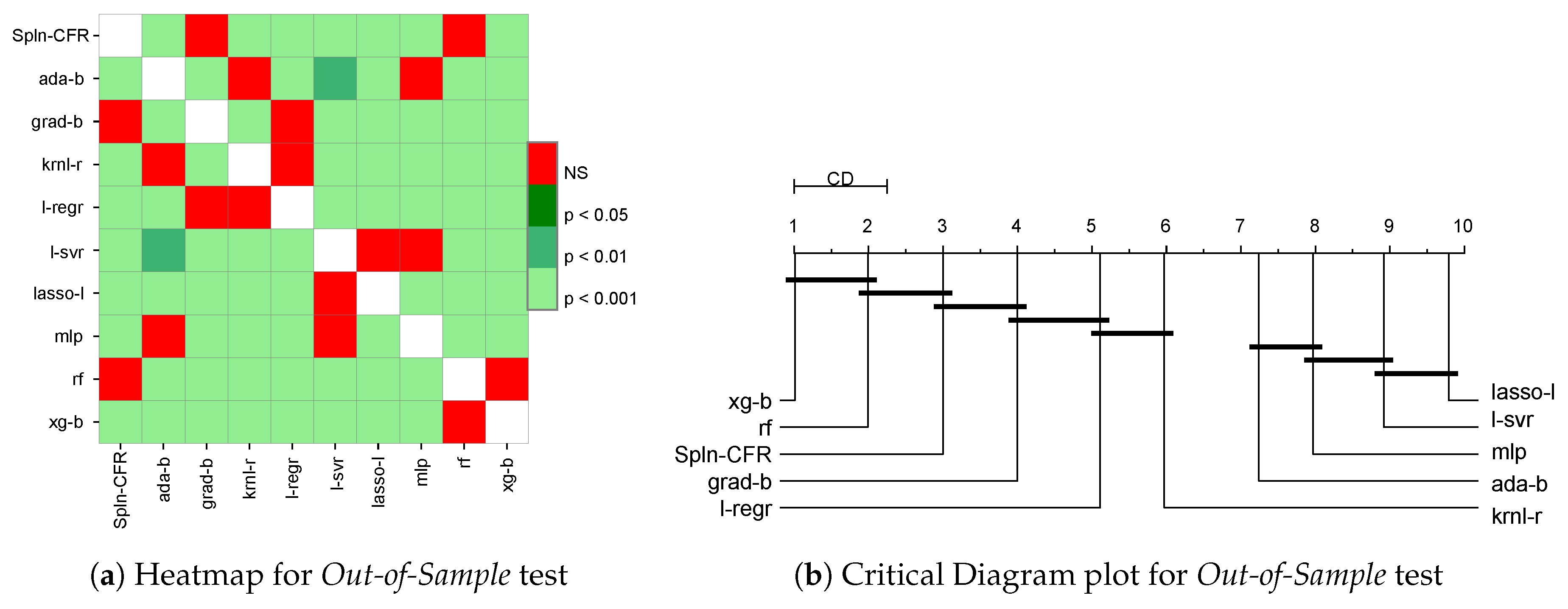
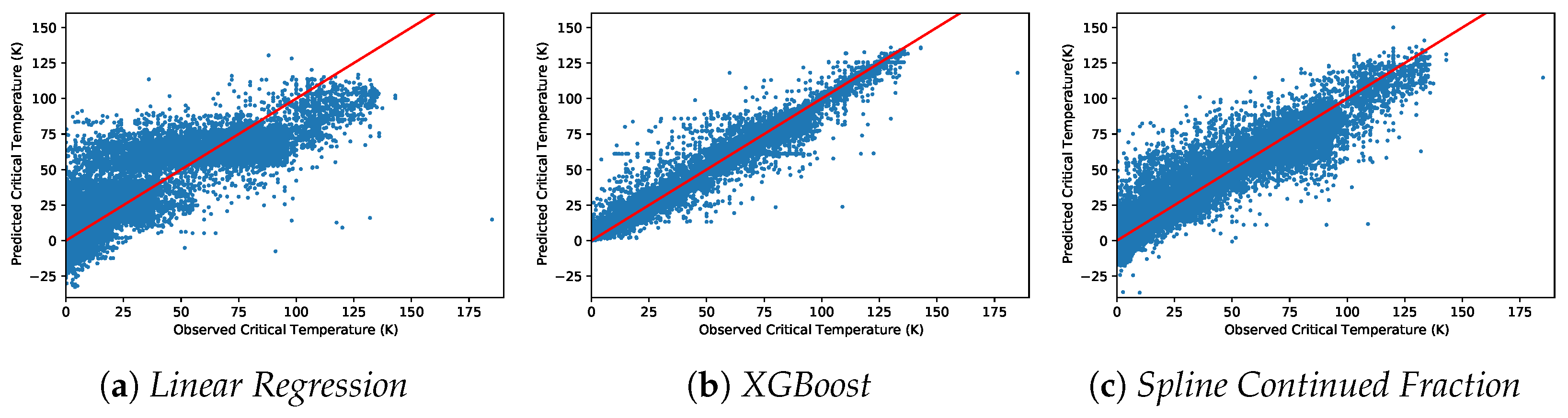
We conducted two main studies to assess the generalization capabilities of many regression algorithms. We denote these as Out-of-Sample and Out-of-Domain, respectively. For the Out-of-Sample study, the data were randomly partitioned into two thirds training data and one third test data. Each model was fitted to the training data, and the RMSE was calculated on the separated test portion of the data.

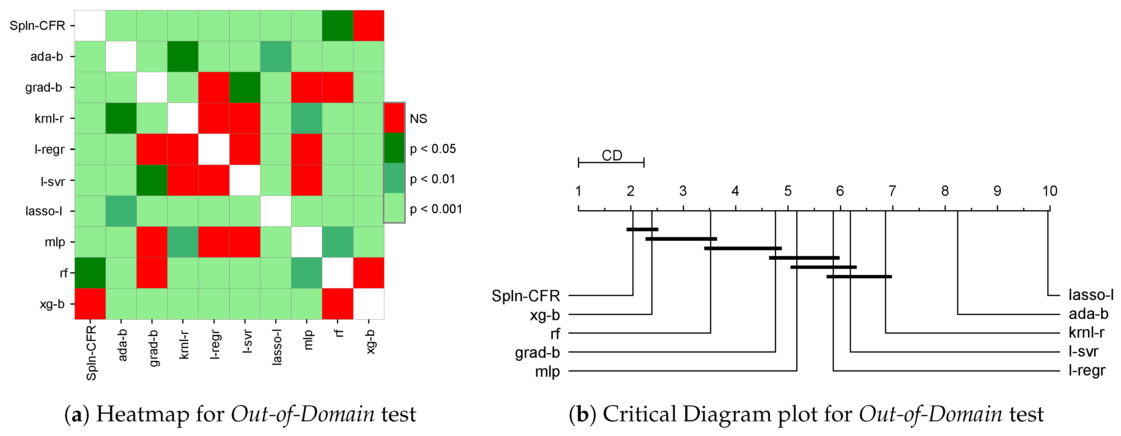
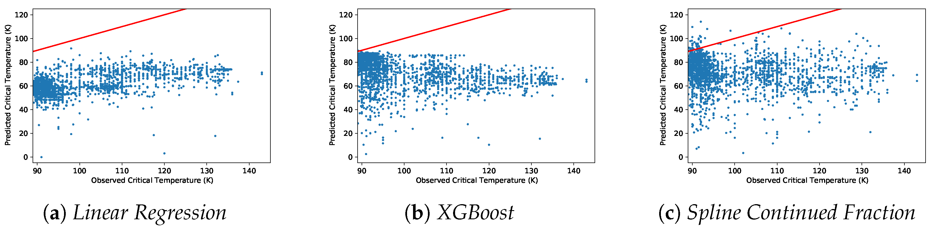
For the Out-of-Domain study, the data were partitioned such that the training samples were always extracted from the set of samples with the lowest 90% of critical temperatures. For the test set, the samples come from the highest 10% of critical temperatures. It turned out that the lowest 90% had critical temperatures < 89 K, whereas the highest 10% had temperatures greater than or equal to 89 K that ranged from 89 K to 185 K (we highlight that the range of variation of the test set is more than that of the training set, making the generalization task a challenging one). For each of the 100 repeated runs of the Out-of-Domain test, we randomly took half of the training set (from lowest 90% of the observed value) to train the models and the same ratio from the test data (from 10% of the highest actual value) to estimate the model performance. The Out-of-Domain study allowed us to assess the capacity of several regression models in terms of “prediction” on a set of materials with higher critical temperatures, meaning that in this case generalization is strictly connected to the extrapolation capacity of the fitted models. We executed both the Out-of-Sample and Out-of-Domain tests 100 times to help validate our conclusions with statistical results.

The Spline Continued Fraction model had a depth of 5, five knots per depth, a normalization constant of 1000, and a regularization parameter $\lambda$ of 0.5. These parameters resulted from a one-dimensional nonlinear model fitting to problems such as the gamma function with noise (already discussed in Figure 1) and others, such as fitting the function $f\left(x\right)=sin\left(x\right)/x$. The parameters were selected empirically using these datasets; no problem-specific tuning on the superconductivity datasets was conducted.

The final model was then iteratively produced by beginning at a depth of 1 and increasing the depth by one until the error was greater than that observed for a previous depth (which we considered as a proxy for overfitting the data).

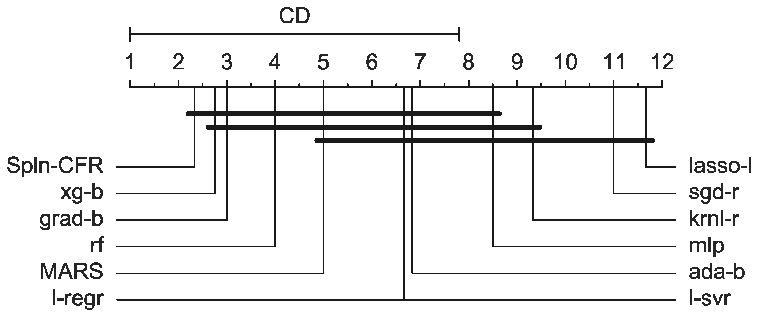
To evaluate the performance of the Spline Continued Fraction (Spln-CFR) introduced in this paper with other state-of-the-art regression methods, we used a set of eleven regressors from two popular Python libraries, namely, the XGBoost [17] and Scikit-learn [18] machine learning libraries. The names of the regression methods are listed as follows:

• AdaBoost (ada-b)
• Gradient Boosting (grad-b)
• Kernel Ridge (krnl-r)
• Lasso Lars (lasso-l)
• Linear Regression (l-regr)
• Linear SVR (l-svr)
• MLP Regressor (mlp)
• Random Forest (rf)
• Stochastic Gradient Descent (sgd-r)
• XGBoost (xg-b)

The XGBoost code is available as an open-source package (https://github.com/dmlc/xgboost, accessed on 11 September 2020). The parameters of the XGBoost model were the same as those used in Hamidieh (2018) [7]. We kept the parameters of the other machine learning algorithms the same as the Scikit defaults.

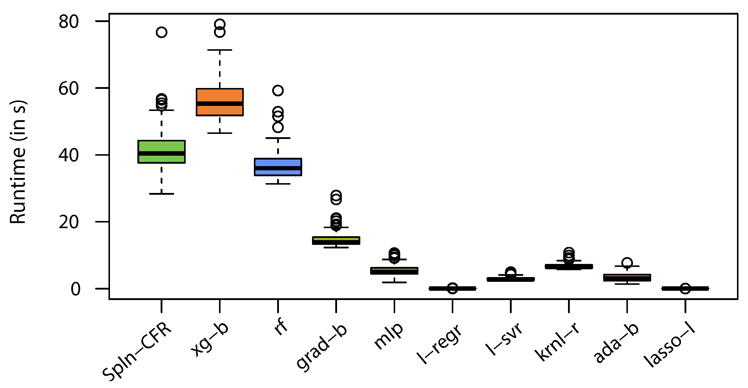
All executions of the experiments were performed on an Intel${}^{\circledR }$ Core${}^{\mathrm{TM}}$ i7-9750H hexcore-based computer with hyperthreading and 16 GB of memory running a Windows 10 operating system. We used Python v3.7 to implement the Spline Continued Fraction using the pyGAM [19] package. All experiments were executed under the same Python runtime and computing environment.

3. Results

Table 1. Results from 100 runs of the proposed Spline Continued Fraction and ten regression methods all trained on the same dataset, with the median of the Root Mean Squared Error (RMSE) and standard deviation as the uncertainty of error.

Regressor	Median RMSE Score ± Std
	Out-of-Sample	Out-of-Domain
Spln-CFR	10.989 ± 0.382	36.327 ± 1.187
xg-b	9.474 ± 0.190	37.264 ± 0.947
rf	9.670 ± 0.197	38.074 ± 0.751
grad-b	12.659 ± 0.178	39.609 ± 0.619
l-regr	17.618 ± 0.187	41.265 ± 0.466
krnl-r	17.635 ± 0.163	41.427 ± 0.464
mlp	19.797 ± 5.140	41.480 ± 9.640
ada-b	18.901 ± 0.686	47.502 ± 0.743
l-svr	26.065 ± 7.838	47.985 ± 1.734
lasso-l	34.234 ± 0.267	74.724 ± 0.376
sgd-r 1	N.R.	N.R.

¹ The Stochastic Gradient Descent Regressor (sgd-r) without parameter estimation predicted unreasonable high values and had an extreme predicted error measure. Hence, we do not report (N.R.) the performance of sgd-r, and have omitted it from further analysis.

presents the results of the regression methods along with with those of the Spline Continued Fraction approach for both the Out-of-Sample and Out-of-Domain studies. The median RMSE value obtained from 100 runs is taken as the Out-of-Sample RMSE estimate.

For each of the 100 repeated runs of the Out-of-Domain test, we estimate the model performance via the Out-of-Domain RMSE score. The median RMSE score obtained from this test performance is reported in Table 1 as Out-of-Domain RMSE. In addition, we report other descriptive statistics, such as the number of times that the regressor correctly predicted a material to have a critical temperature greater or equal to 89 K.

3.1. Out-of-Sample Test

For the Out-of-Sample testing, XGBoost achieved the lowest error (median RMSE score of 9.47) among the eleven regression methods. The three closest regression methods to XGBoost are Random Forest (median RMSE of 9.67), Spline Continued Fraction (median RMSE of 10.99), and Gradient Boosting (median RMSE of 12.66). Stochastic Gradient Descent without parameter estimation performed the worst among all regression methods used in the experiment, and due to the unreasonable high error observed in the runs we have omitted it from further analysis.

Statistical Significance of the Results of the Out-of-Sample Test

To evaluate the significance of the results obtained by the different regression methods for the Out-of-Sample test, we applied a Friedman test for repeated measure [20] for the 100 runs. We computed the ranking of the methods for each of the runs based on the RMSE score obtained in the test distribution of the Out-of-Sample settings. This helps to determine whether the experiment’s techniques were consistent in terms of performance. The statistical test found a p-value = 1.9899e-183, which rejects the null hypothesis, i.e., “all the algorithms perform the same”; thus, we proceeded with the post hoc test.

We applied Friedman’s post hoc test on the ranking of the ten regressors computed for the RMSE scores obtained for 100 runs of the Out-of-Sample test. In Figure 2a, the p-values obtained for the test are plotted as a heat map. It can be seen that there exist no significant differences (NS) between the performances of Spline Continued Fraction (Spnl-CFR) and those of rf and grad-b.

Additionally, we generated the Critical Difference (CD) diagram proposed in [21] to visualize the differences among the regressors for their median ranking. The CD plot uses the Nyemeni post hoc test and places the regressors on the x-axis of their median ranking. It then computes the critical difference of the rankings between them and connects those which are closer than the critical difference with a horizontal line, denoting them as statistically ‘non-significant’.

We plot the CD graph in Figure 2b using the implementation from the Orange data mining toolbox [22] in Python. The Critical Difference (CD) is found to be $1.25$. It can be seen that xg-b ranked first among the regressors, with no significant difference’, while rf ranked second. The median ranking of the proposed Spline Continued Fraction was third, withno significant differences in the performance rankings of rf and grad-b.

3.2. Out-of-Domain Test

For the task of Out-of-Domain prediction, the Spline Continued Fraction regressor exhibited the best performance (median RMSE score of 36.3) among all regression methods used in the experiment (in Table 1). The three closest regressors to the proposed Spline Continued Fraction method are XGBoost (median RMSE = 37.3), Random Forest (median RMSE = 38.1), and Gradient Boosting (median RMSE = 39.6).

3.2.1. Statistical Significance of the Results of the Out-of-Domain Test

To test the significance of the results obtained by the different regression methods for the Out-of-Domain study, we employed the same statistical test used above for the Out-of-Sample study. The test returned a p-value = 1.2065e-156, rejecting the null hypothesis; thus, we proceeded with the post hoc test.

The p-values obtained for the post hoc test are plotted as a heat map in Figure 3a for the Out-of-Domain test. It can be seen that no significant differences (NS) exist between the performance of Spline Continued Fraction (Spnl-CFR) and those of Random Forest (rf) and XGBoost (xg-b). There is no significant difference between the performance ranking of Linear Regression (l-regr) and those of mlp, l-svr, krnl-r, and grad-b.

The Critical Difference (CD) graph for the Out-of-Domain test is plotted in Figure 3b. The Critical Difference (CD) is $1.3898$. It is evident from the critical difference plot that the top three methods in Out-of-Domain prediction are Spline Continued Fraction, XGBoost, and Random Forest. It can be seen that the average ranking of Spln-CFR is very close to second, which is the best-ranking performance among the ten regressors. There is no significant difference between Spline Continued Fraction and the second-best method, XGBoost (xg-b), which has an average ranking between second and third for Out-of-Domain prediction.

3.2.2. Runtimes of the Different Methods on the Out-of-Domain Test

Figure 4 shows the running time (in s) required by each of the regression methods for 100 runs of the Out-of-Domain test. It can be seen that the lowest required running times are for Linear Regression, with a 50th percentile runtime of 0.02 s and maximum of 0.158 s, and Lasso Lars, with a 50th percentile runtime of 0.013 s and maximum of 0.027 s. XGBoost (xg-b) required the longest time (50th percentile runtime of 55.33 s and maximum 79.05 s); on the other hand, Random Forest and the proposed Spline Continued Fraction regression required very similar times (50th percentile runtimes of 36.88 s and 41.65 s for rf and Spln-CFR, respectively) on the Out-of-Domain test.

4. Discussion

To illustrate the performance of models in the Out-of-Sample study, we employed Linear Regression, XGBoost, and Spline Continued Fraction on the training set and plotted the predictions versus the actual temperatures for the entire dataset (in Figure 5). We were able to reproduce the results of the Out-of-Sample test from Hamidieh [7] Figure 5a, with an RMSE of 17.7. The Out-of-Sample models for Spline Continued Fraction and XGBoost were used to predict the critical temperature for the entire dataset. Together, the figures show that Spln-CFR performed better in modelling Out-of-Sample critical temperatures than Linear Regression, particularly for larger temperatures.

Figure 6 shows the actual versus predicted critical temperature for the Out-of-Domain test for the Linear Regression, XGBoost, and Spline Continued Fraction models. Recall that in the Out-of-Domain test settings we trained each of the models with the samples from the bottom 90% of the observed temperature, which is < 89 K, and measured the samples’ test performance using the top 10% of the observed critical temperatures, with 2126 samples in the test set.

Another set of our observed results are interesting for discussion and might be relevant for future research directions. In

Table 2. Predicted vs. actual critical temperatures for the materials with the top twenty predicted temperatures in the Out-of-Domain study, i.e., the one in which the lowest 90% of critical temperature samples were used for drawing the training data. The average values of the critical temperatures ($\overline{x}$), the average relative error ($\overline{\eta }$), and the root mean squared error (RMSE, denoted as rm) of these materials for the top twenty predictions (which are not necessarily the same, as they depend on the models) are shown in the last rows. 

Spln-CFR		xg-b		rf		grad-b		mlp		l-regr		l-svr		krnl-r		ada-b		lasso-l
y	pred	y	pred	y	pred	y	pred	y	pred	y	pred	y	pred	y	pred	y	pred	y	pred
92.00	114.14	89.20	89.64	91.19	87.89	89.50	83.44	109.00	100.81	98.00	91.59	112.00	94.81	98.00	91.02	89.50	58.63	89.00	27.06
90.00	109.69	94.20	89.19	89.90	87.88	89.90	83.44	124.90	100.31	112.00	89.14	100.00	93.49	112.00	88.67	89.50	58.63	89.00	27.06
111.00	108.54	89.88	88.69	90.00	87.88	90.50	83.44	114.00	99.70	105.00	87.53	132.60	93.49	105.00	86.84	89.70	58.63	89.00	27.06
93.50	108.01	89.93	88.34	90.20	87.88	91.50	83.44	128.40	99.59	117.00	87.06	105.00	92.94	117.00	86.65	89.80	58.63	89.00	27.06
99.00	106.50	90.00	88.15	90.90	87.88	90.00	83.42	127.40	99.53	100.00	85.92	115.00	92.93	100.00	85.88	89.80	58.63	89.00	27.06
105.60	105.01	90.10	88.15	91.00	87.88	91.80	83.42	127.80	99.53	132.60	85.92	111.00	92.90	132.60	85.88	89.90	58.63	89.00	27.06
113.00	104.35	91.00	88.15	92.00	87.88	90.00	82.22	130.10	98.76	115.00	85.50	110.00	92.84	115.00	85.51	90.00	58.63	89.00	27.06
113.00	103.95	91.30	88.15	92.20	87.88	89.50	79.29	128.50	98.55	111.00	84.97	106.70	92.54	111.00	84.46	90.00	58.63	89.00	27.06
106.60	103.95	96.10	88.15	92.40	87.88	90.00	79.29	128.40	98.45	132.00	84.96	126.90	91.73	132.00	84.42	90.50	58.63	89.00	27.06
128.70	103.92	90.00	88.10	92.50	87.88	91.00	79.29	128.80	98.45	110.00	84.31	117.00	91.73	110.00	84.38	91.50	58.63	89.00	27.06
91.80	102.10	91.40	88.10	92.74	87.88	91.80	79.29	131.40	98.33	106.70	83.95	126.80	91.30	106.70	82.97	100.00	58.63	89.00	27.06
108.00	101.56	92.60	87.82	92.80	87.88	92.30	79.29	128.80	98.10	126.90	82.72	115.00	90.84	95.00	82.64	108.00	58.63	89.00	27.06
92.00	101.32	91.60	87.53	93.00	87.88	90.00	78.85	128.70	93.96	105.00	82.63	95.00	90.80	105.00	82.01	110.00	58.63	89.00	27.06
90.00	101.19	93.00	87.53	93.00	87.88	91.60	78.85	130.30	93.94	95.00	82.62	121.60	90.80	107.00	81.88	110.90	58.63	89.00	27.06
105.10	100.50	93.80	87.49	93.05	87.88	89.10	78.79	131.30	93.93	107.00	82.47	100.00	90.78	126.90	81.82	114.00	58.63	89.00	27.06
130.30	100.35	89.90	87.48	93.20	87.88	89.20	78.79	122.00	91.96	105.00	82.41	107.00	90.78	105.00	81.51	114.00	58.63	89.00	27.06
93.00	100.24	90.00	87.48	93.40	87.88	89.40	78.79	123.50	91.64	126.80	82.12	90.00	90.63	90.00	81.40	116.00	58.63	89.10	27.06
91.50	100.00	90.20	87.48	93.50	87.88	89.40	78.79	121.00	90.69	98.50	82.03	96.00	90.49	126.80	81.24	122.50	58.63	89.10	27.06
91.50	99.18	90.90	87.48	91.80	87.75	89.40	78.79	115.00	90.14	112.00	82.03	128.70	90.48	117.00	80.89	127.00	58.63	89.10	27.06
116.00	98.39	91.00	87.48	92.10	87.69	89.50	78.79	110.00	90.01	117.00	81.83	130.30	90.26	121.60	80.87	130.90	58.63	89.10	27.06
$\overline{x}$: 103.08	103.64	91.31	88.03	92.044	87.86	90.27	80.49	124.47	96.32	111.63	84.59	112.33	91.83	111.68	84.05	102.68	58.63	89.02	27.06
$\overline{\eta }$:	0.1085	0.036		0.0453		0.1083		0.224		0.2351		0.1733		0.2389		0.4187		0.696
rm:	13.6023	3.7753		4.3261		10.0078		28.9783		29.3265		23.9282		30.2426		46.2473		61.96

, we report the top twenty predicted versus actual (y) temperatures for all ten regression methods for a single run of the Out-of-Domain test. The last row of the table shows the averages of the corresponding actual critical temperatures for the materials with the highest twenty predicted values by each of the models. Interestingly, XGBoost’s top twenty predictions of the critical temperature are all below 90 K (in the range of 87.48 to 89.64 K). Similarly, Random Forest’s top twenty predictions are in the range of 87.69 to 87.89 K. The top twenty predicted critical temperatures by the Linear Regression are in the range of 81.83 to 91.59 K. In contrast, the top twenty predicted critical temperatures by Spline Continued Fraction vary from 98.39 to 114.14 K, which by comparison represents the highest starting and ending values among all the regressors. We report the average temperature ($\overline{x}$), average relative errors ($\overline{\eta }$), and RMSE score for the top twenty predictions. XGBoost shows the lowest value for both $\overline{\eta }$ (0.036) and RMSE ($3.775$) among the ten regressors. In terms of those scores, our proposed Spln-CFR is in the fourth position. However, looking at the average of the predictions, Spln-CFR has the highest average prediction temperatures for the top twenty predictions on the Out-of-Domain test.

Because all the actual critical temperatures of the test set in the Out-of-Domain settings were $\ge 89$ K, it is relevant to evaluate for how many of these samples each regression method was able to predict above that value. Here, we consider the predicted value as P = critical temperature value$\ge 89$ K (denoted as ‘P’ for positive) and N = critical temperature value < 89 K (denoted as ‘N’ for negative). In

Table 3. Number of times the different methods predicted a critical temperature value $T_c\ge 89$ K (denoted as ‘P’ for positive) and $T_c<89$ K (denoted as ‘N’ for Negative) on the Out-of-Domain test.

Regressor	Out-of-Domain Predicted Critical Temperature, ${\mathit{T}}_{\mathit{c}}$
	P (${\mathit{T}}_{\mathit{c}}$ $\ge 89$ K)	N (${\mathit{T}}_{\mathit{c}}$ < 89 K)
Spln-CFR	108	2018
xg-b	2	2124
rf	0	2126
grad-b	0	2126
mlp	21	2105
l-regr	2	2124
l-svr	34	2092
krnl-r	1	2125
ada-b	0	2126
lasso-l	0	2126

, we report the number of samples for which each of the methods predicted a temperature value in the P and N categories for the whole testing set of the Out-of-Domain test. It can be seen that only six regression methods predicted the critical temperature of $\ge 89$ K for at least one sample. Both Linear Regression and XGBoost predicted two sample temperatures with the critical temperature $\ge 89$ K. Kernel Ridge predicted only one sample value within that range, while MLP Regressor and Linear SVR predicted it for 21 and 34 samples, respectively. The proposed Spline Continued Fraction predicted 108 sample values of $\ge 89$ K, the best among all regression methods used in our experiments.

We examined the consensus between the regression methods in Out-of-Domain predictions. Only five regressors, (Spln-CFR, xg-b, mlp, l-regr, l-svr, and krnl-r), were able to predict at least one positive value (critical temperature $\ge 89$ K). We computed pairwise inter-rater agreement statistics, Cohen’s kappa [23], for these five regression methods. We tabulated the value of Kappa ($\kappa$) ordered by highest to lowest; the level of agreement is outlined in

Table 4. Inter-rater agreement between the pairs of regressor methods where the resulting models were able to predict at least one positive temperature value ($T_c\ge 89$ K).

Rater 1	Rater 2	Value of Kappa ($\mathit{\kappa }$)	Level of Agreement
Spln-CFR	xg-b	−0.001851	No Agreement
Spln-CFR	mlp	0.030476	None to Slight
Spln-CFR	l-regr	0.016365	None to Slight
Spln-CFR	l-svr	0.104988	None to Slight
Spln-CFR	krnl-r	−0.000933	No Agreement
xg-b	mlp	−0.001721	No Agreement
xg-b	l-regr	−0.000942	No Agreement
xg-b	l-svr	−0.001780	No Agreement
xg-b	krnl-r	−0.000628	No Agreement
mlp	l-regr	−0.001721	No Agreement
mlp	l-svr	0.208516	Fair
mlp	krnl-r	−0.000899	No Agreement
l-regr	l-svr	0.053874	None to Slight
l-regr	krnl-r	0.666457	Substantial
l-svr	krnl-r	−0.000915	No Agreement

. It can be seen that in most cases there is either no agreement (nine cases) none to slight (four cases) between the pairs of regressors. Such behaviour is seen in the agreement between the pairs formed with Spln-CFR and each of the other five methods. MLP Regressor and Linear SVR have fair agreement in their predictions. The highest value is $\kappa =0.67$ for Linear Regression and Kernel Ridge, yielding substantial agreement.

Extrapolation Capability of the Regressors in General

As all of the results presented in this work are for a special case of finding models for the extrapolation of the critical temperature of superconductors, we included more robust experimental outcomes with a set of six datasets used in [8]. This additional test can help to evaluate the extrapolation capabilities of the regressors in other problem domains.

Jerome Friedman proposed a Multivariate Adaptive Regression Splines (MARS) algorithm in [24] which aggregates multiple linear regression models throughout the range of target values. We used the implementation of the MARS algorithm from the py-earth Python library (https://contrib.scikit-learn.org/py-earth/content.html#multivariate-adaptive-regression-splines accessed on 8 October 2021). We included a comparison of MARS with Spln-CFR and other regressors to assess their extrapolation capability.

Here, the samples from each of the datasets were sorted based on the target value, which was then split into the out-of-domain setting by taking samples with the lower 90% target values for training and the higher 10% target values for testing. We took half of the samples uniformly and at random from the out-of-domain training set to build the model and uesd the same ratio from the out-of-domain test set for prediction for each of the 100 independent runs. We applied min-max normalization on the training set and used the same distribution to normalize the test set.

We analyze the regressors’ performance statistically in Figure 7; it can be seen that MARS has a median ranking of fifth and is statistically significantly different from only krnl-r, sgd-r, and lasso-l. On the other hand, the proposed Spln-CFR achieves the first rank among all the methods, with a median ranking between two to three. To calculate how many predictions surpass the threshold (which matches the highest target score in the training data) in out-of-domain scenarios, we can convert the predictions of each model back to their original scale, i.e., denormalize them.

Table 5. Number of predictions by the different regressor methods which fall within the out-of-domain threshold range for the test set during 100 repeated runs on six datasets from [8].

Regressor	in Range	Regressor	in Range	Regressor	in Range
Spln-CFR	13,560	grad-b	1227	ada-b	0
MARS	3716	mlp	1158	lasso-l	0
l-regr	2594	xg-b	826	rf	0
l-svr	2045	krnl-r	735	sgd-r	0

shows the full denormalization results. These counts show that Spln-CFR has the highest number of predictions (13,560), followed by MARS (3716) and l-regr (2594). These results demonstrate the strength of the regressors in terms of their extrapolation capability.

5. Conclusions

To conclude, we provide a brief summary of the results observed using this new technique:

• For the Out-of-Sample study, the proposed Spln-CFR approach is among the top three methods based on the median RMSE obtained for 100 independent runs (Table 1).
• For the statistical test of the Out-of-Sample rankings, Spln-CFR is statistically similar to the second-ranked method, Random Forest, in Figure 2b.
• In terms of the Out-of-Domain median RMSE obtained for 100 runs, Spln-CFR is ranked first (Table 1).
• For the statistical test of the Out-of-Domain rankings in Figure 3b, Spln-CFR is the best method, with a median ranking close to second, and is statistically similar to the second-best regressor, XGBoost, which has a median ranking between second and third.
• Spln-CFR correctly predicted 108 unique materials with critical temperature values greater than or equal to 89 K in the Out-of-Domain test, nearly twice the number achieved all the other regression methods combined, which was 60 (Table 3).

Table 2 reveals interesting characteristics of the different methods that deserve further consideration as an area of research. First, it can be noted that the twenty top materials for the different methods are not necessarily the same, although a few intersections obviously exist. In the Out-of-Domain study, the top twenty predicted critical temperature values by Spln-CFR were all above 98.9 K, with eighteen being above 100 K. The average RMSE critical temperature on this set (103.64 K) is nearly the same as the predicted one (103.08 K). The RMSE of xg-b, however, is nearly three times smaller, while the method’s top predictions are materials with relatively smaller values (average of 91.31 K). For the collected information of the materials in the dataset, we observed that the top suggestions of critical temperatures in superconductors are closer to the measured temperatures, at least on the average, when using Spln-CFR. Therefore, the use of Spln-CFR as a surrogate model to explore the possibility of testing the superconductivity of materials may provide better returns.

Interestingly, while we observed similarities in the behavior of xg-b and other multivariate regression techniques, there were important differences worth noting. For instance, Linear Regression, perhaps the simplest scheme of them all, shows interesting behavior; its top twenty highest predictions are all in the range of 81.83–91.59 K while the actual values are in the interval 98.00–132.60 K. For the multi-layer perceptron method (mlp), the top twenty highest predictions are all in the range of 90.01–100.81 K, yet the true values are in the interval 109.00–131.40 K. By considering the rankings given to several materials, as opposed to the predicted values, valuable information about materials can be obtained with these techniques when trained using the MSE, allowing prioritization of materials for testing.

Overall, our results show the limitations of the current dataset. One limitation is the lack of other useful molecular descriptors that can provide important problem domain knowledge about the structure of the materials and their properties. In addition, careful segmentation of the different materials may be necessary. In a sense, the results of our experiments an help the AI community to reflect on how to carry out such analyses and provide motivation for closer collaboration with superconductivity specialists in order to provide other molecular descriptors.

The inherent difficulties in prediction using in this dataset can be compared to other areas in which some of us have been working extensively, such as the prediction of survivability in breast cancer using transcriptomic data. In both cases, the obtained models showed poor generalization capability when the training samples were not separated into meaningful subgroups. One reason that our continued fraction-based method may be achieving better results on the generalization test in our Out-of-Domain study may be that there are structural similarities in the set of compounds used to define the continued fraction approximation at the highest temperatures in the training set. Thus, perhaps indirectly, useful information exists in the molecular descriptors present in these samples which the continued fraction representation approach is able to exploit. We will investigate this hypothesis further in a future publication, where we will additionally aim to include more relevant problem domain information in collaboration with specialists in order to benefit from the structure and known properties of the actual compounds.

In terms of future research on the algorithm we propose here, it is clear that Spln-CFR is already a promising approach with obvious extensions worth considering in the future. For instance, the inclusion of the bagging and boosting techniques could improve its Out-of-Sample performance, while modifications of the MSE used in the training set may lead to better learning performance in the Out-of-Domain scenario. We plan to conduct further research in these areas.

Note Added in Proof

As of 29 July 2023, while completing the last version of this manuscript before publication, a group of Korean researchers has made an intriguing announcement. They claim to have discovered a material known as LK-99, which they assert is the world’s first room temperature and ambient pressure superconductor. The details of this discovery were made available in preprints on Saturday, 22 July 2023, at 07:51:19 UTC [25] and 10:11:28 UTC [26].

The scientific community worldwide is closely monitoring this breakthrough with great anticipation. Notably, the authors of the above publications suggest that the critical temperature of LK-99 might exceed 400 degrees Kelvin [25], a value significantly surpassing any previous expectations derived from the existing dataset from Hamidieh [7]. If their claims are validated and other laboratories can reproduce the results, it will not undermine our ongoing pursuit of enhanced generalization through multivariate regression extrapolation.

On the contrary, if proven correct, this remarkable discovery may provide valuable insights into the study of effective extrapolation regression methods, especially in combination with the screening of chemically novel compositions described in the forthcoming paper by Seegmiller et al. [27]. In light of the considerable attention now focused on these matters globally, we foresee a significant surge in the importance of multivariate regression techniques for material discovery. We eagerly await the unfolding developments in this exciting field.

References

1. Tinkham, M. Introduction to Superconductivity: International Series in Pure and Applied Physics; McGraw-Hill: New York, NY, USA, 1975. [Google Scholar]
2. Tinkham, M. Introduction to Superconductivity, 2nd ed.; Courier Corporation: Chelmsford, MA, USA, 2004. [Google Scholar]
3. Liu, W.; Li, S.; Wu, H.; Dhale, N.; Koirala, P.; Lv, B. Enhanced superconductivity in the Se-substituted 1T-PdTe2. Phys. Rev. Mater. 2021, 5, 014802. [Google Scholar] [CrossRef]
4. Chen, X.; Wu, T.; Wu, G.; Liu, R.; Chen, H.; Fang, D. Superconductivity at 43 K in SmFeAsO(1−x)Fx. Nature 2008, 453, 761–762. [Google Scholar] [CrossRef] [PubMed] [Green Version]
5. Zhang, Y.; Liu, W.; Zhu, X.; Zhao, H.; Hu, Z.; He, C.; Wen, H.H. Unprecedented high irreversibility line in the nontoxic cuprate superconductor (Cu, C)Ba2Ca3Cu4O(11+). Sci. Adv. 2018, 4, eaau0192. [Google Scholar] [CrossRef] [PubMed] [Green Version]
6. Liu, W.; Lin, H.; Kang, R.; Zhu, X.; Zhang, Y.; Zheng, S.; Wen, H.H. Magnetization of potassium-doped p-terphenyl and p-quaterphenyl by high-pressure synthesis. Phys. Rev. B 2017, 96, 224501. [Google Scholar] [CrossRef] [Green Version]
7. Hamidieh, K. A data-driven statistical model for predicting the critical temperature of a superconductor. Comput. Mater. Sci. 2018, 154, 346–354. [Google Scholar] [CrossRef] [Green Version]
8. Sun, H.; Moscato, P. A Memetic Algorithm for Symbolic Regression. In Proceedings of the IEEE Congress on Evolutionary Computation, CEC 2019, Wellington, New Zealand, 10–13 June 2019; IEEE: New York, NY, USA, 2019; pp. 2167–2174. [Google Scholar] [CrossRef]
9. Moscato, P.; Sun, H.; Haque, M.N. Analytic Continued Fractions for Regression: A Memetic Algorithm Approach. Expert Syst. Appl. 2021, 179, 115018. [Google Scholar] [CrossRef]
10. Moscato, P.; Cotta, C. An Accelerated Introduction to Memetic Algorithms. In Handbook of Metaheuristics; Gendreau, M., Potvin, J.Y., Eds.; Springer International Publishing: Cham, Switzerland, 2019; pp. 275–309. [Google Scholar] [CrossRef]
11. Moscato, P.; Mathieson, L. Memetic Algorithms for Business Analytics and Data Science: A Brief Survey. In Business and Consumer Analytics: New Ideas; Moscato, P., de Vries, N.J., Eds.; Springer: Berlin/Heidelberg, Germany, 2019; pp. 545–608. [Google Scholar] [CrossRef]
12. Moscato, P.; Haque, M.N.; Moscato, A. Continued fractions and the Thomson problem. Sci. Rep. 2023, 13, 7272. [Google Scholar] [CrossRef] [PubMed]
13. Sun, S.; Ouyang, R.; Zhang, B.; Zhang, T.Y. Data-driven discovery of formulas by symbolic regression. Mater. Res. Soc. Bull. 2019, 44, 559–564. [Google Scholar] [CrossRef]
14. Backeljauw, F.; Cuyt, A.A.M. Algorithm 895: A continued fractions package for special functions. ACM Trans. Math. Softw. 2009, 36, 15:1–15:20. [Google Scholar] [CrossRef]
15. Boor, C.D. A Practical Guide to Splines; Springer: New York, NY, USA, 1978; Volume 27. [Google Scholar]
16. Hastie, T.; Tibshirani, R.; Friedman, J. The Elements of Statistical Learning; Springer: Berlin/Heidelberg, Germany, 2009; pp. 139–190. [Google Scholar]
17. Chen, T.; Guestrin, C. XGBoost: A Scalable Tree Boosting System. In Proceedings of the KDD ’16: 22nd ACM SIGKDD International Conference on Knowledge Discovery and Data Mining, San Francisco, CA, USA, 13–17 August 2016; pp. 785–794. [Google Scholar] [CrossRef] [Green Version]
18. Pedregosa, F.; Varoquaux, G.; Gramfort, A.; Michel, V.; Thirion, B.; Grisel, O.; Blondel, M.; Prettenhofer, P.; Weiss, R.; Dubourg, V.; et al. Scikit-learn: Machine Learning in Python. J. Mach. Learn. Res. 2011, 12, 2825–2830. [Google Scholar]
19. Servén, D.; Brummitt, C. pyGAM: Generalized Additive Models in Python. Available online: https://doi.org/10.5281/zenodo.1208723 (accessed on 18 April 2022).
20. Friedman, M. The use of ranks to avoid the assumption of normality implicit in the analysis of variance. J. Am. Stat. Assoc. 1937, 32, 675–701. [Google Scholar] [CrossRef]
21. Demšar, J. Statistical comparisons of classifiers over multiple data sets. J. Mach. Learn. Res. 2006, 7, 1–30. [Google Scholar]
22. Demšar, J.; Curk, T.; Erjavec, A.; Gorup, V.; Hočevar, T.; Milutinovič, M.; Možina, M.; Polajnar, M.; Toplak, M.; Starič, A.; et al. Orange: Data Mining Toolbox in Python. J. Mach. Learn. Res. 2013, 14, 2349–2353. [Google Scholar]
23. Cohen, J. A coefficient of agreement for nominal scales. Educ. Psychol. Meas. 1960, 20, 37–46. [Google Scholar] [CrossRef]
24. Friedman, J.H. Multivariate adaptive regression splines. Ann. Stat. 1991, 19, 1–67. [Google Scholar] [CrossRef]
25. Lee, S.; Kim, J.H.; Kwon, Y.W. The First Room-Temperature Ambient-Pressure Superconductor. arXiv 2023, arXiv:2307.12008. [Google Scholar]
26. Lee, S.; Kim, J.; Kim, H.T.; Im, S.; An, S.; Auh, K.H. Superconductor Pb10−xCux(PO4)6O showing levitation at room temperature and atmospheric pressure and mechanism. arXiv 2023, arXiv:2307.12037. [Google Scholar]
27. Seegmiller, C.C.; Baird, S.G.; Sayeed, H.M.; Sparks, T.D. Discovering chemically novel, high-temperature superconductors. Comput. Mater. Sci. 2023, 228, 112358. [Google Scholar] [CrossRef]
Figure 1. Examples of the fit obtained by the Spline Continued Fraction using a dataset generated thanks to the gamma function with added noise. We present several continued fractions with depths of 3 (a), 5 (b), 10 (c), and 15 (d). In this example, the number of knots k was chosen to be 3, n o r m = 1, and λ = 0.1.
Algorithms 16 00382 g001
Figure 2. Statistical comparison of the regressors for the Out-of-Sample test: (a) heat map showing the significance levels of the p-values obtained by the Friedman post hoc test and (b) critical difference (CD) plot showing the statistical significance of the rankings achieved by the different regression methods.
Algorithms 16 00382 g002
Figure 3. Statistical comparison of the regressors for the Out-of-Domain test: (a) heat map showing the significance levels of the p-values obtained by the Friedman post hoc test and (b) critical difference (CD) plot showing the statistical significance of the rankings achieved by the different regression methods.
Algorithms 16 00382 g003
Figure 4. Runtime (in seconds) required for model building and prediction by the regressors for 100 runs of the Out-of-Domain test, in which samples with the lowest 90% of critical temperatures were drawn as the training data and an equal number of samples drawn from the top 10% highest critical temperatures constituted the test data.
Algorithms 16 00382 g004
Figure 5. Out-of-Sample test results, showing the predicted vs. actual temperatures for the entire dataset with regression models trained on the training data: (a) Linear Regression (replicating the outcome from Hamidieh), (b) XGBoost, and (c) Spline Continued Fraction.
Algorithms 16 00382 g005
Figure 6. Out-of-Domain test results, showing the predicted vs. actual temperatures of the samples for the highest 10% of critical temperatures, where the models were fitted using the samples with the lowest 90% critical temperatures. The x-axis values up to 145 K are shown, leaving one extreme value (185 K) outside of the visualized area. Results of the Out-of-Domain test for: (a) Linear Regression, with an RMSE of 41.3; (b) XGBoost, with an RMSE of 36.3; and (c) Spline Continued Fraction, with an RMSE of 34.8.
Algorithms 16 00382 g006
Figure 7. Critical difference (CD) plot showing the statistical significance of rankings achieved by the regression methods for 100 runs on the six datasets form [8].
Algorithms 16 00382 g007