Article

Risk-Sensitive Policy with Distributional Reinforcement Learning

1
Department of Electrical Engineering and Computer Science, University of Liège, 4031 Liège, Belgium
2
Information Processing and Communications Laboratory, Institut Polytechnique de Paris, 91120 Paris, France
*
Author to whom correspondence should be addressed.
Algorithms 2023, 16(7), 325; https://doi.org/10.3390/a16070325
Submission received: 14 June 2023 / Revised: 23 June 2023 / Accepted: 23 June 2023 / Published: 30 June 2023
(This article belongs to the Topic Intelligent Systems and Robotics)

Abstract

:
Classical reinforcement learning (RL) techniques are generally concerned with the design of decision-making policies driven by the maximisation of the expected outcome. Nevertheless, this approach does not take into consideration the potential risk associated with the actions taken, which may be critical in certain applications. To address that issue, the present research work introduces a novel methodology based on distributional RL to derive sequential decision-making policies that are sensitive to the risk, the latter being modelled by the tail of the return probability distribution. The core idea is to replace the Q function generally standing at the core of learning schemes in RL by another function, taking into account both the expected return and the risk. Named the risk-based utility function U, it can be extracted from the random return distribution Z naturally learnt by any distributional RL algorithm. This enables the spanning of the complete potential trade-off between risk minimisation and expected return maximisation, in contrast to fully risk-averse methodologies. Fundamentally, this research yields a truly practical and accessible solution for learning risk-sensitive policies with minimal modification to the distributional RL algorithm, with an emphasis on the interpretability of the resulting decision-making process.

1. Introduction

The reinforcement learning (RL) approach is concerned with the learning process of a sequential decision-making policy based on the interactions between an agent and its environment [1]. More precisely, the training is based on the rewards acquired by the agent from the environment as a consequence of its actions. Within this context, the objective is to identify the actions maximising the discounted sum of rewards, also named return. Multiple sound approaches exist, based on the RL paradigm, and key successes/milestones have been achieved throughout the years of research. Nevertheless, these RL algorithms mostly rely on the expectation of the return, not on its complete probability distribution. For instance, the popular Q-learning methodology is based on the modelling of the Q function, which can be seen as an estimation of the expected return [2].
While focusing exclusively on the expectation of the return has already proven to be perfectly sound for numerous applications, this approach exhibits clear limitations for other decision-making problems. Indeed, some areas of application may also require properly mitigating the risk associated with the actions taken [3]. One could, for instance, mention the healthcare [4] and finance [5] sectors, but also robotics in general [6], and especially autonomous driving [7]. For the sake of clarity, two concrete examples are provided as illustrations. In finance, during a trading activity in a market, the objective is not to solely maximise profit but also to properly monitor and mitigate the risk. In robotics, when navigating in an environment, a robot has to ensure that its decision-making will not induce an excessive level of risk, which could potentially harm its integrity. This concern holds true in diverse environments, ranging from the harsh and inhospitable conditions of planet Mars to everyday scenarios like autonomous driving on roads. In fact, there a myriad of sequential decision-making problems exist, which require an appropriate evaluation and mitigation of the risk. Furthermore, such a requirement for risk management may not only be true for the decision-making policy, but potentially also for the exploration policy during the learning process. In addition, properly taking risk into consideration may be particularly convenient in environments characterised by substantial uncertainty.
This research work suggests taking advantage of the distributional RL approach, belonging to the Q-learning category, in order to learn risk-sensitive policies. Basically, a distributional RL algorithm targets the complete probability distribution of the random return rather than only its expectation [8]. This methodology presents key advantages. Firstly, it enables the learning of a richer representation of the environment, which may lead to an increase in the decision-making policy performance. Secondly, the distributional RL approach contributes to improving the explainability of the decision-making process, which is key in machine learning to avoid black-box models. Lastly and most importantly for this research work, it makes possible the convenient derivation of decision-making policies, as well as exploration strategies that are sensitive to the risk.
The core idea promoted by this research work is the use of the risk-based utility function U as a replacement for the popular Q function for action selection. In fact, it may be seen as an extension of the Q function that considers the risk, which is assumed to be represented by the worst returns that are achievable by a policy. Therefore, the function U is to be derived from the complete probability distribution of the random return Z, which is learnt by any distributional RL algorithm. The single modification to that RL algorithm to learn risk-sensitive policies is to employ the utility function U rather than the expected return Q for both exploration and decision-making. This enables the presented approach to become a very practical and interpretable RL solution for risk-sensitive decision making.

2. Literature Review

The core objective of the classical RL approach is to learn optimal decision-making policies without any concerns about the risk or safety [1]. The resulting policies are said to be risk-neutral. Nevertheless, there are numerous real-world applications requiring to take the risk into consideration in order to ensure safer decision making [3]. Two main approaches can be identified to achieving a safe RL. Firstly, the optimality criterion can be modified so that a safety factor is included. Secondly, the exploration process can be altered based on a risk metric [9]. These techniques give rise to risk-sensitive or risk-averse policies.
Scientific research on risk-sensitive RL has been particularly active for the past decade. Various relevant risk criteria have been studied for that purpose. The most popular ones are undoubtedly the mean-variance [10,11,12] and the (Conditional) Value at Risk (CVaR) [13,14,15]. Innovative techniques have been introduced for both policy gradient [16,17,18] and value iteration [19,20,21,22,23] approaches, with the proposed solutions covering both discrete and continuous action spaces. Additionally, risk-sensitive methodologies have also been studied in certain niche sub-fields of RL, such as robust adversarial RL [24], but also multi-agent RL [25].
Focusing on the value iteration methodology, the novel distributional RL approach [8] has been a key breakthrough, by providing access to the full probability distribution of the random return. For instance, [20] suggests achieving risk-sensitive decision-making via a distortion risk measure. Applied on top of the IQN distributional RL algorithm, this is, in fact, equivalent to changing the sampling distribution of the quantiles. In [21], a novel actor-critic framework is presented, based on the distributional RL approach for the critic component. The latter work is extended to the offline setting in [22], since training RL agents online may be prohibitive because of the risk inevitably induced by exploration. Additionally, [23] introduces the Worst-Case Soft Actor Critic (WCSAC) algorithm, which is based on the approximation of the probability distribution of accumulated safety-costs in order to achieve risk control. More precisely, a certain level of CVaR, estimated from the distribution, is regarded as a safety constraint.
In light of this literature, the novel solution introduced in this research paper presents key advantages. Firstly, the methodology proposed is relatively simple and can be applied on top of any distributional RL algorithm with minimal modifications to the core algorithm. Secondly, the proposed approach can span the entire potential trade-off between risk minimisation and expected return maximisation. According to the user’s needs, the policy learnt can be risk-averse, risk-neutral or in between the two (risk-sensitive). Lastly, the solution presented improves the interpretability of the decision-making policy that was learnt.

3. Materials and Methods

3.1. Theoretical Background

3.1.1. Markov Decision Process

In RL, the interactions between the agent and its environment are generally modelled as a Markov decision process (MDP). An MDP is a 6-tuple ( S , A , p R , p T , p 0 , γ ) where S and A , respectively, are the state and action spaces, p R ( r | s , a ) is the probability distribution from which the reward r R is drawn given a state–action pair ( s , a ) , p T ( s | s , a ) is the transition probability distribution, p 0 ( s 0 ) is the probability distribution over the initial states s 0 S , and γ [ 0 , 1 ] is the discount factor. The RL agent makes decisions according to its policy π : S A , which is assumed to be deterministic, mapping the states s S to the actions a A .

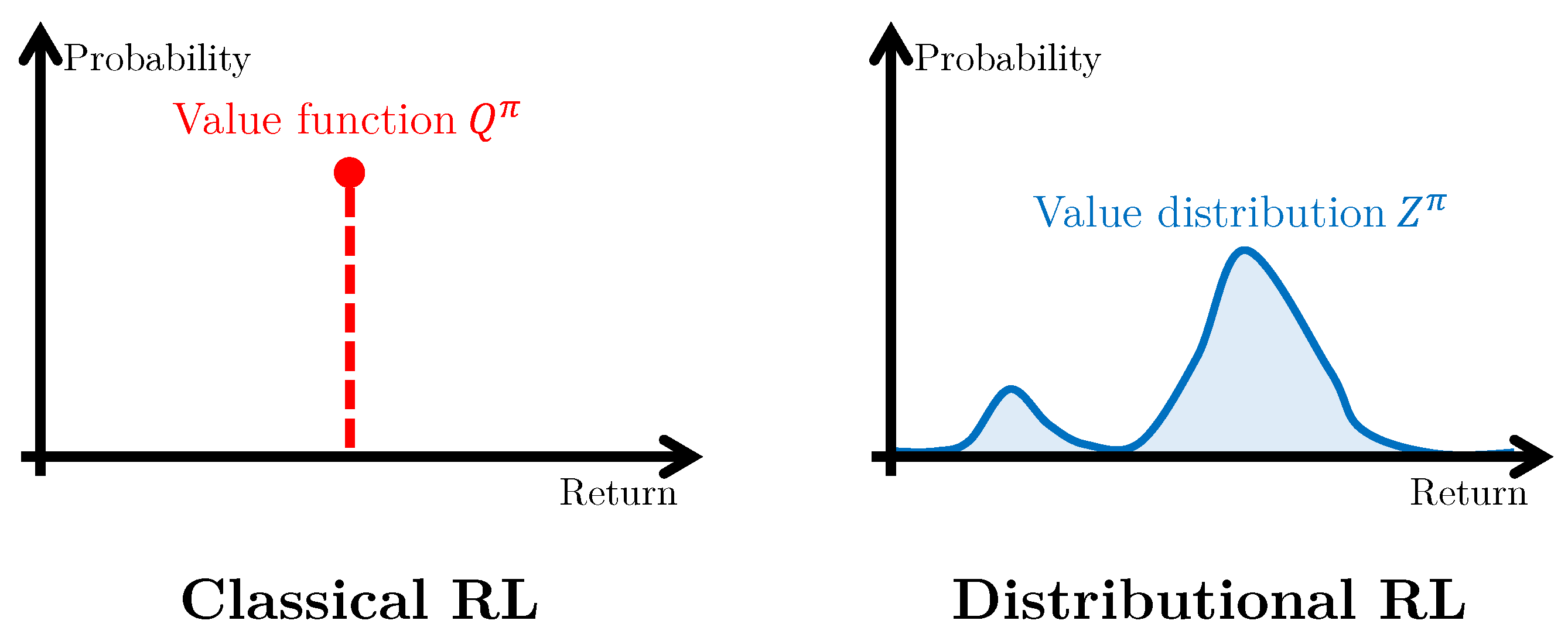
3.1.2. Distributional Reinforcement Learning

In classical Q-learning RL, the core idea is to model the state–action value function  Q π : S × A R of a policy π . This important quantity Q π ( s , a ) represents the expected discounted sum of rewards obtained by executing an action a A in a state s S and then following a policy π :
Q π ( s , a ) = E s t , r t t = 0 γ t r t , ( s 0 , a 0 ) : = ( s , a ) , a t = π ( s t ) .
The key to the learning process is the Bellman equation [26] that the Q function satisfies:
Q π ( s , a ) = E s , r r + γ Q π ( s , π ( s ) ) .
In classical RL, the main objective is to determine an optimal policy  π * , which can be defined based on the optimal state–action value function  Q * : S × A R , as follows:
Q * ( s , a ) = E s , r r + γ max a A Q * ( s , a ) ,
π * ( s ) argmax a A Q * ( s , a ) .
The optimal policy π * maximises the expected return (discounted sum of rewards). This research work later presents an alternative objective criterion for optimality in a risk-sensitive RL setting.
The distributional RL approach goes a step further by modelling the full probability distribution over returns instead of only its expectation [8], as illustrated in Figure 1. To this end, let the reward R ( s , a ) be a random variable distributed under p R ( · | s , a ) , the state-action value distribution  Z π Z of a policy π (also called state-action return distribution function) is a random variable, defined as follows:
Z π ( s , a ) = D t = 0 γ t R ( s t , a t ) , ( s 0 , a 0 ) : = ( s , a ) , a t = π ( s t ) , s t + 1 p T ( · | s t , a t ) ,
where A = D B denotes the equality in probability distribution between the random variables A and B. Therefore, the state–action value function Q π is the expectation of the random return  Z π . Equivalent to the expected case, there exists a distributional Bellman equation that recursively describes the random return Z π of interest:
Z π ( s , a ) = D R ( s , a ) + γ P π Z π ( s , a ) ,
P π Z π ( s , a ) : = D Z π ( s , a ) , s p T ( · | s , a ) , a = π ( s ) ,
where P π : Z Z is the transition operator. To end this section, one can define the distributional Bellman operator  T π : Z Z , together with the distributional Bellman optimality operator  T * : Z Z as follows:
T π Z π ( s , a ) = D R ( s , a ) + γ P π Z π ( s , a ) ,
T * Z * ( s , a ) = D R ( s , a ) + γ Z * s , π * ( s ) , s p T ( · | s , a ) .
A distributional RL algorithm may be characterised by two core features. Firstly, both the representation and parameterisation of the random return probability distribution have to be properly selected. Multiple solutions exist representing a unidimensional distribution: probability density function (PDF), cumulative distribution function (CDF), quantile function (QF). In practice, deep neural networks (DNNs) are generally used for the approximation of these particular functions. The second key feature relates to the probability metric adopted for comparing two distributions, such as the Kullback–Leibler (KL) divergence, the Cramer distance or the Wasserstein distance. More precisely, the role of the probability metric in distributional RL is to quantitatively compare two probability distributions of the random return so that a temporal difference (TD) learning method is applied in a similar way to the mean squared error between Q-values in classical RL. The probability metric plays an even more important role, as different metrics offer distinct theoretical convergence guarantees for distributional RLs.

3.2. Methodology

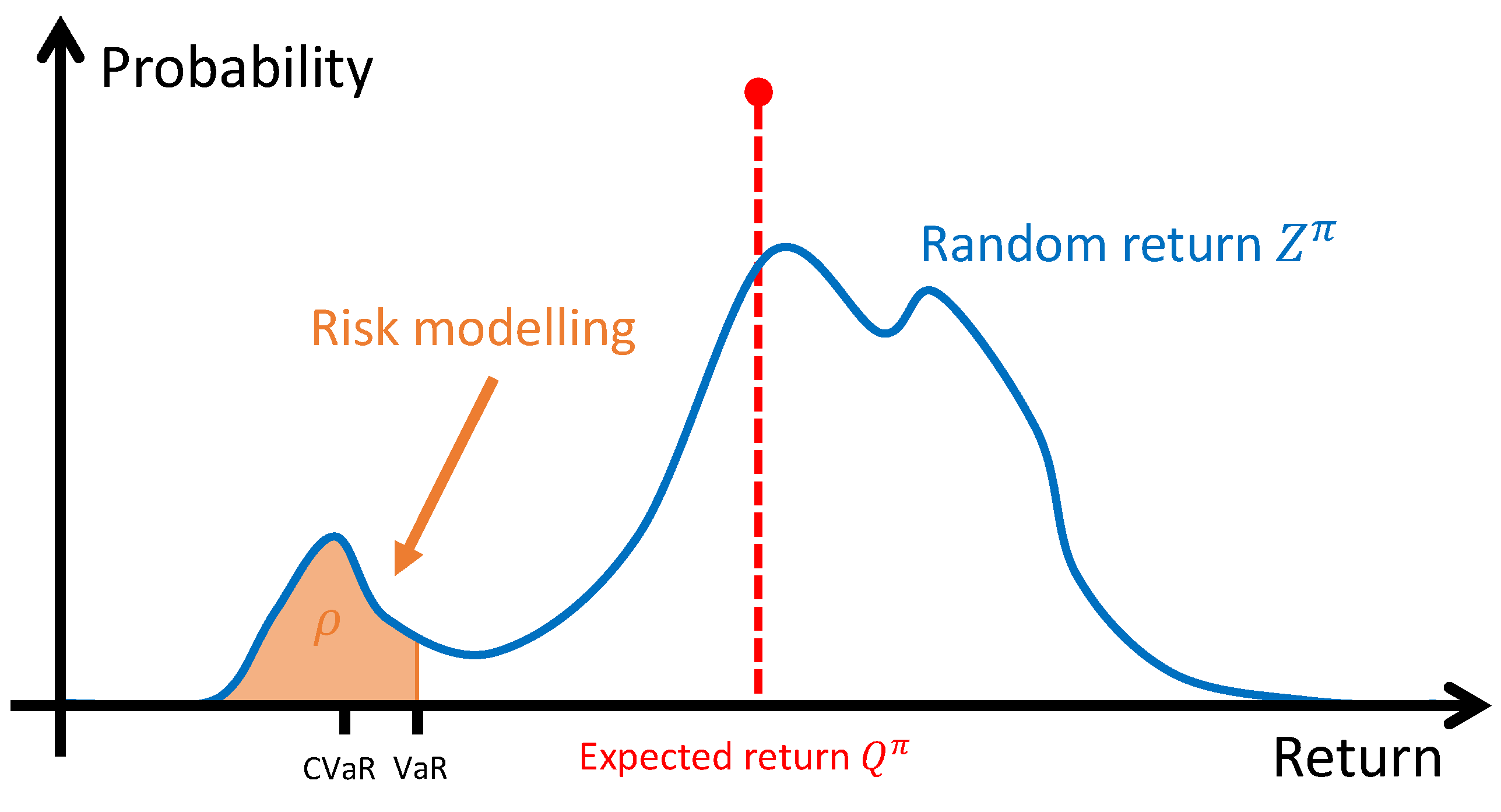
3.2.1. Objective Criterion for Risk-Sensitive RL

As previously explained, the objective in classical RL is to learn a decision-making policy π Π that maximises the expectation regarding the discounted sum of rewards. Formally, this objective criterion can be expressed as the following:
maximise π E t = 0 γ t r t .
In order to effectively take into consideration the risk and value its mitigation, this research work presents an update for the former objective. In fact, coming up with a generic definition for the risk is not trivial since the risk is generally dependent on the decision-making problem itself. In the present research work, it is assumed that the risk is assessed on the basis of the worst returns achievable by a policy π . Therefore, a successful decision-making policy should ideally maximise the expected discounted sum of rewards while avoiding low values for the worst-case returns. The latter requirement is approximated with a new constraint attached to the former objective, defined in Equation (10): the probability of having the policy achieving a lower return than a certain minimum value should not exceed a given threshold. Mathematically, the alternative objective criterion proposed for risk-sensitive RL can be expressed as follows:
maximise π E t = 0 γ t r t , such that p t = 0 γ t r t R min ϵ ,
where:
p [ ] denotes the probability of the event ⋆,
R min is the minimum acceptable return (from the perspective of risk mitigation),
ϵ [ 0 , 1 ] is the threshold probability that is not to be exceeded.

3.2.2. Practical Modelling of the Risk

As previously hinted, this research work assumes that the risk associated with an action is related to the worst achievable returns when executing that particular action and then following a certain decision-making policy π . In such a context, the distributional RL approach becomes particularly interesting, by providing access to the full probability distribution of the random return Z π . Thus, the risk can be efficiently assessed by examining the so-called tail of the learnt probability distribution. Moreover, the new constraint in Equation (11) can be approximated through popular risk measures such as the Value at Risk and Conditional Value at Risk. Illustrated in Figure 2, these two risk measures are formally expressed as follows:
VaR ρ ( Z π ) = inf z R : F Z π ( z ) ρ ,
CVaR ρ ( Z π ) = E z | z VaR ρ ( Z π ) ,
where F Z π represents the CDF of the random return Z π .
More generally, the present research work introduces the state-action risk function  R π : S × A R of a decision-making policy π , which is the equivalent of the Q function for the risk. More precisely, that function R π ( s , a ) quantifies the riskiness of the discounted sum of rewards obtained by executing an action a A in a state s S and then following policy π :
R π ( s , a ) = R ρ Z π ( s , a ) ,
where:
R ρ : Z R 
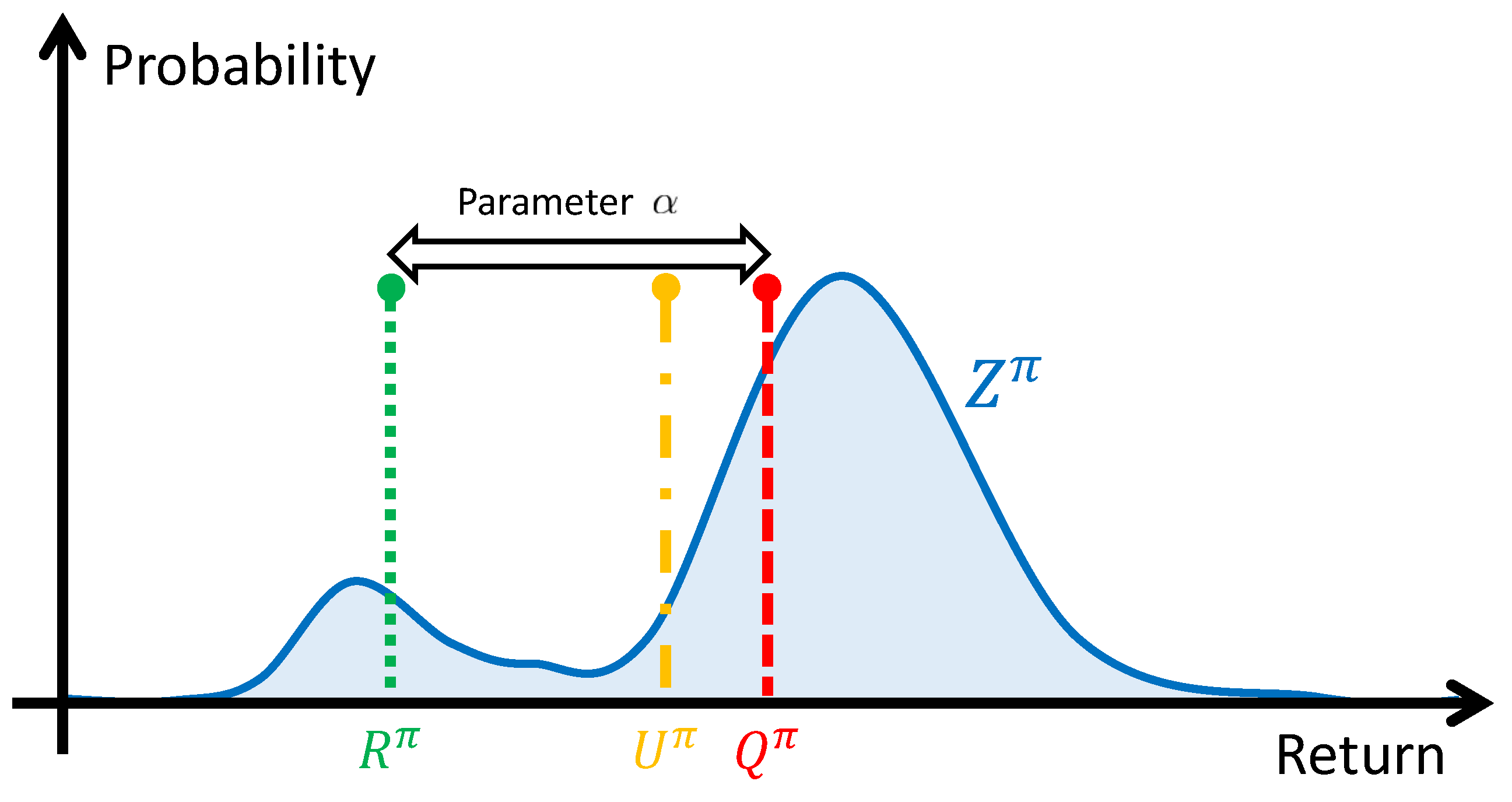
is a function extracting risk features from the random return probability distribution Z π , such as VaR ρ or CVaR ρ ,
ρ 0 , 1 is a parameter corresponding to the cumulative probability associated with the worst returns, generally between 0 % and 10 % . In other words, this parameter controls the size of the random return distribution tail from which the risk is estimated.

3.2.3. Risk-Based Utility Function

In order to pursue the objective criterion defined in Equation (11) for risk-sensitive RL, this research work introduces a new concept: the state-action risk-based utility function. Denoted U π ( s , a ) , the utility function assesses the quality of an action a A in a certain state s S in terms of expected performance and risk, assuming that the policy π is followed afterwards. In fact, the intent is to extend the popular Q function so that the risk is taken into consideration by taking advantage of the risk function defined in Section 3.2.2. More precisely, the utility function U π is built as a linear combination of the Q π and R π functions. Formally, the risk-based utility function U π : S × A R of a policy π is defined as the following:
U π ( s , a ) = α Q π ( s , a ) + ( 1 α ) R π ( s , a )
= α E Z π ( s , a ) + ( 1 α ) R ρ Z π ( s , a ) ,
where α 0 , 1 is a parameter controlling the trade-off between expected performance and risk. If α = 0 , the utility function will be maximised with a fully risk-averse decision-making policy. On the contrary, if α = 1 , the utility function degenerates into the Q function quantifying the performance on expectation. Figure 3 graphically describes the utility function U π , which moves along the x-axis between the quantities R π and Q π when modifying the value of the parameter α .

3.2.4. Risk-Sensitive Distributional RL Algorithm

In most applications, the motivation for choosing the distributional RL approach over the classical one is related to the improved expected performance that results from learning a richer representation of the environment. Despite having access to the full probability distribution of the random return, only the expectation is exploited to derive decision-making policies:
π ( s ) argmax a A E Z π ( s , a ) Q π ( s , a ) .
Nevertheless, as previously hinted, the random return Z π also contains valuable information about the risk, which could be exploited to learn risk-sensitive decision-making and exploration policies. The present research work suggests that risk-sensitive distributional RL should be achieved by maximising the utility function U π , derived from Z π , instead of the expected return Q π when selecting actions. This alternative operation would be performed during both exploration and exploitation. Even though maximising the utility function is not exactly equivalent to the optimisation of the objective criterion defined in Equation (11), it is a relevant step towards risk-sensitive RL. Consequently, a risk-sensitive policy π can be derived as follows:
π ( s ) argmax a A U π ( s , a ) .
Throughout the learning phase, a classical Q-learning algorithm is expected to progressively converge towards the optimal value function Q * that naturally arises from the optimal policy π * . In a similar way, the proposed risk-sensitive RL algorithm jointly learns the optimal policy π * and the optimal state-action risk-based utility function  U * . More formally, the latter two are mathematically defined as the following:
U * ( s , a ) = α E Z * ( s , a ) + ( 1 α ) R ρ Z * ( s , a ) ,
Z * ( s , a ) = D R ( s , a ) + γ Z * s , π * ( s ) ,
π * ( s ) argmax a A U * ( s , a ) .
The novel methodology proposed by this research work to learn risk-sensitive decision-making policies based on the distributional RL approach is summarised as follows. Firstly, select any distributional RL algorithm that learns the full probability distribution of the random return Z π . Secondly, leave the learning process unchanged except for action selection, which involves the maximisation of the utility function U π rather than the expected return Q π . This adaptation is the single change to the distributional RL algorithm, occurring at two different locations within the algorithm: i. the generation of new experiences by interacting with the environment, ii. the learning of the random return Z π based on the distributional Bellman equation. However, this adaptation has no consequence on the random return Z π learnt by the distributional RL algorithm, only on the actions derived from that probability distribution. Algorithm 1 details the proposed solution in a generic way, with the required modifications highlighted.

3.3. Performance Assessment Methodology

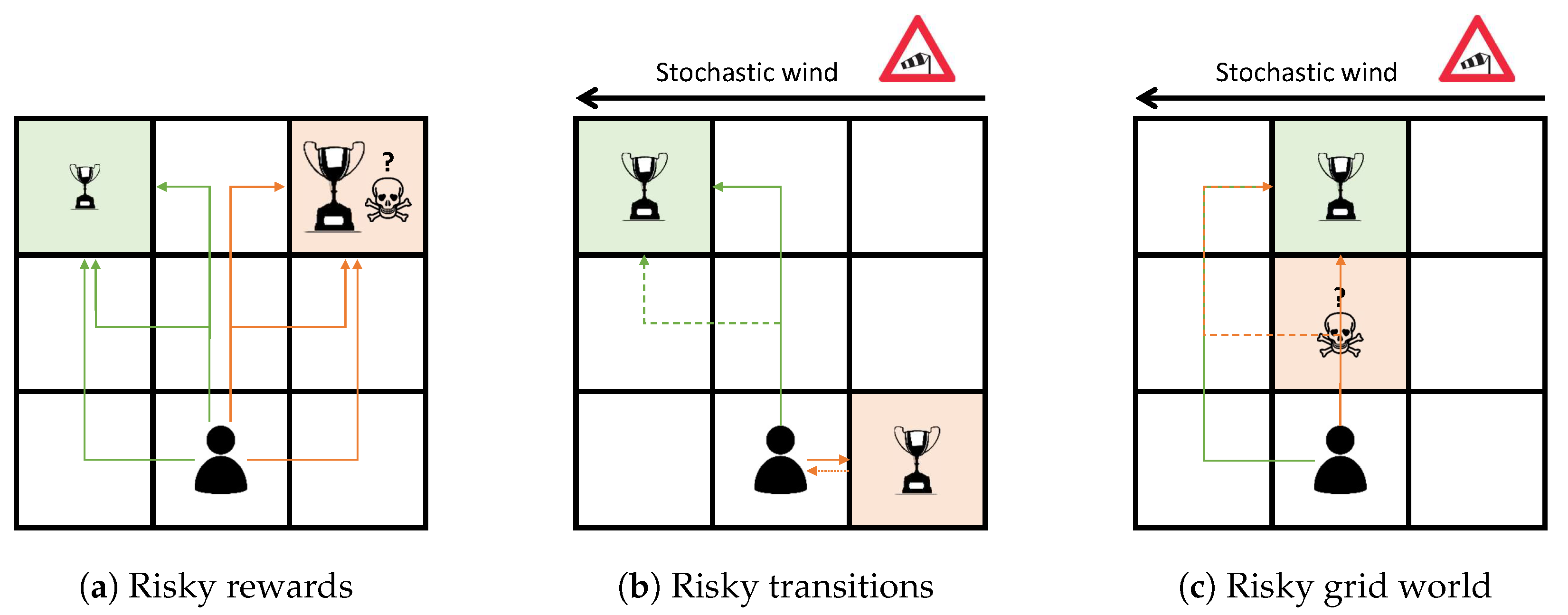
3.3.1. Benchmark Environments

This research work introduces some novel benchmark environments in order to assess the soundness of the proposed methodology to design risk-sensitive policies based on the distributional RL approach. These environments consist of three toy problems that are specifically designed to highlight the importance of considering the risk in a decision-making policy. More precisely, the control problems are built in such a way that the optimal policy will differ depending on whether the objective is to solely maximise the expected performance or to also mitigate the risk. This is achieved by including relevant stochasticity in both the state transition function p T and reward function p R . Moreover, the benchmark environments are designed to be relatively simple in order to ease the analysis and understanding of the decision-making policies tha tare learnt. This simplicity also ensures the accessibility of the experiments, since distributional RL algorithms generally require a considerable amount of computing power. Figure 4 illustrates these three benchmark environments, and highlights the optimal paths to be learnt depending on the objective being pursued. For the sake of completeness, a thorough description of the underlying MDPs is provided in Appendix A, including the stochastic reward and transition functions.
Algorithm 1 Risk-sensitive distributional RL algorithm.
  • Initialise the experience replay memory M of capacity C.
  • Initialise both the main and target DNN weights θ = θ .
  • for episode = 0 to N do
  •    for time step t = 0 to T, or until episode termination do
  •      Acquire the state s from the environment E .
  •      With probability ϵ , select a random action a A .
  •      Otherwise, select the action a = argmax a A U π ( s , a ; θ ) .
  •      Execute action a in environment E to get the next state s and the reward r.
  •      Store the experience e = ( s , a , r , s ) in M.
  •      Randomly sample from M a minibatch of N e experiences e i = ( s i , a i , r i , s i ) .
  •      for  i = 0 to N e  do
  •         Distributional Bellman equation:
  •                 Z π ( s i , a i ; θ ) = D r i + γ Z π ( s i + 1 , argmax a i A U π ( s i + 1 , a i ; θ ) ; θ ) .
  •      end for
  •      Compute the resulting loss L ( θ ) , according to the probability metric selected.
  •      Update the main DNN parameters θ using a deep learning optimiser with learning rate L r .
  •      Update the target DNN parameters θ = θ every N steps.
  •      Anneal the ϵ -greedy exploration parameter ϵ .
  •    end for
  • end for
The first benchmark environment is named risky rewards. It consists of a 3 × 3 grid world, within which an agent has to reach one of two objective areas that are equidistant from its fixed initial location. The difficulty of this control problem lies in the choice of the objective area to target, because of the stochasticity present in the reward function. Reaching the first objective area yields a reward with a lower value in expectation and a limited deviation from that average. On the contrary, reaching the second objective location yields a reward that is higher in expectation, at the cost of an increased risk.
The second benchmark environment that was studied is named risky transitions. It consists of a 3 × 3 grid world, within which an agent has to reach one of two objective areas as quickly as possible in the presence of a stochastic wind. The agent is initially located in a fixed area that is very close to an objective, but the required move to reach it is in opposition to the wind direction. Following that path results in a reward that is higher in expectation, but there is a risk to be repeatedly countered, caused by the stochastic wind. On the contrary, the longer path is safer but yields a lower reward on average.
The last presented benchmark environment is named risky grid world. This control problem can be viewed as a combination of the two previously described environments since it integrates both stochastic rewards and transitions. It consists of a 3 × 3 grid world within which an agent, initially located in a fixed area, has to reach a fixed objective location as quickly as possible. To achieve that goal, three paths are available. The agent may choose the shortest path to the objective location, characterised by a stochastic trap, or get around this risky situation by taking a significantly longer route. This bypass can be made from the left or from the right, another critical choice in terms of risk because of the stochastic wind. Once again, the optimal path is dependent on the objective criterion being pursued.

3.3.2. Risk-Sensitive Distributional RL Algorithm Analysed

The distributional RL algorithm selected to assess the soundness of the methodology introduced to learn risk-sensitive decision-making policies is the Unconstrained Monotonic Deep Q-Network with Cramer (UMDQN-C) [27]. Basically, this particular distributional RL algorithm models the CDF of the random return in a continuous way by taking advantage of the Cramer distance to derive the TD-error. Moreover, the probability distributions learnt are ensured to be valid thanks to the specific architecture exploited to model the random return: Unconstrained Monotonic Neural Network (UMNN) [28]. The latter has been demonstrated to be a universal approximator of continuous monotonic functions, which is particularly convenient when representing CDFs. In practice, the UMDQN-C algorithm has been shown to achieve great results, both in terms of policy performance and in terms of random return probability distribution quality. This second feature clearly motivated the selection of this specific distributional RL algorithm to conduct the following experiments, since accurate random return probability distributions are required to properly estimate the risk. The reader can refer to the original research paper [27] for more information about the UMDQN-C distributional RL algorithm.
As previously explained in Section 3.2.2, the presented approach requires the choice of a function R ρ to extract risk features from the random return probability distribution Z π . In the following experiments, Value at Risk (VaR) is adopted to estimate the risk. This choice is motivated by both the popularity of that risk measure in practice and by the efficiency of computation. Indeed, this quantity can be conveniently derived from the CDF of the random return learnt by the UMDQN-C algorithm.
In the next section presenting the achieved results, the risk-sensitive version of the UMDQN-C algorithm is denoted RS-UMDQN-C. The detailed pseudo-code of that new risk-sensitive distributional RL algorithm can be found in Appendix B.
To conclude this section, ensuring the reproducibility of the results in a transparent way is particularly important to this research work. In order to achieve this, Table 1 provides a brief description of the key hyperparameters used in the experiments. Moreover, the entire experimental code is made publicly available at the following link: https://github.com/ThibautTheate/Risk-Sensitive-Policy-with-Distributional-Reinforcement-Learning, accessed on 10 June 2023.

4. Results and Discussion

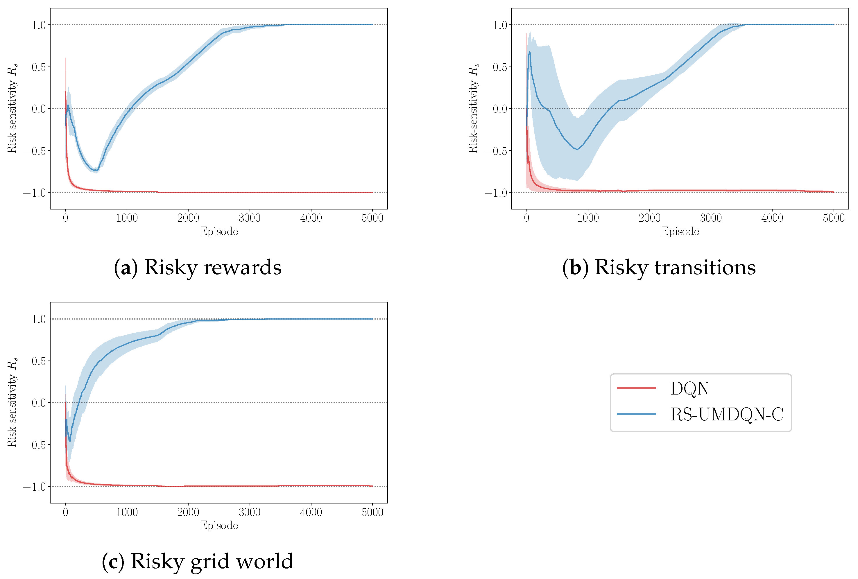
4.1. Decision-Making Policy Performance

To begin with, the performance achieved by the decision-making policies π learnt has to be evaluated, both in terms of expected outcome and risk. For comparison purposes, the results obtained by the well-established DQN algorithm, a reference without any form of risk sensitivity, are presented alongside those of the newly introduced RS-UMDQN-C algorithm. It should be mentioned that these two RL algorithms achieve very similar results when risk sensitivity is disabled ( α = 1 for the RS-UMDQN-C algorithm), as expected.
In the following, two analyses are presented. Firstly, the probability distribution of the cumulative reward of a policy π , denoted S π Z , is investigated. More precisely, the expectation E [ · ] , the risk function R ρ [ · ] and the utility function U [ · ] of that random variable S π are derived for each algorithm and compared. Secondly, this research work introduces a novel easy-to-interpret performance indicator R s [ 1 , 1 ] to evaluate the risk sensitivity of the decision-making policies that are learnt, by taking advantage of the simplicity of the benchmark environments presented in Section 3.3.1. In fact, this is made possible by the easy assessment, from a human perspective, of the relative riskiness of a path in the grid world environments being studied. If the optimal path in terms of risk is chosen (green arrows in Figure 4), a score R s = + 1 is awarded. On the contrary, the riskier path, which is optimal in terms of expectation (orange arrows in Figure 4) yields a score of R s = 1 . If no objective or trap areas are reached within the allowed time, a score of R s = 0 is delivered. Consequently, the evolution of this performance indicator provides valuable information about the convergence of the RL algorithms towards the different possible paths, as well as about the stability of the learning process. Formally, let τ = s t , a t t [ 0 , T ] with s t S and a t A be a trajectory defined over a time horizon T < 10 (ending with a terminal state, and subject to an upper bound), and let τ + and τ , respectively, be the sets of trajectories associated with the green and orange paths in Figure 4. Based on these definitions, the risk sensitivity R s of a policy π is a random variable that can be assessed via Monte Carlo as the following:
R s ( π ) = + 1 if π produces trajectories s t , a t t [ 0 , T ] τ + with a t = π ( s t ) , 1 if π produces trajectories s t , a t t [ 0 , T ] τ with a t = π ( s t ) , 0 otherwise .
The first results regarding policy performance are summarised in Table 2, which compares the decision-making policies learnt by the DQN and RS-UMDQN-C algorithms both in terms of expected outcome and risk. The second results regarding policy performance are compiled in Figure 5, plotting the evolution of the risk-sensitivity performance indicator R s during the training phase. It can be clearly observed from these two analyses that the proposed approach is effective in learning decision-making policies that are sensitive to the risk for relatively simple environments. As expected, the DQN algorithm yields policies that are optimal in expectation, whatever the level of risk incurred. In contrast, the RS-UMDQN-C algorithm is able to leverage both expected outcome and risk in order to learn decision-making policies that produce a slightly lower expected return with a significantly lower risk level. This allows for the proposed methodology to significantly outperform the risk-neutral RL algorithm of reference with respect to the performance indicator of interest U [ S π ] in Table 2. Finally, it is also encouraging to observe from Figure 5 that the learning process seems to be quite stable for simple environments, despite having to maximise a much more complicated function.

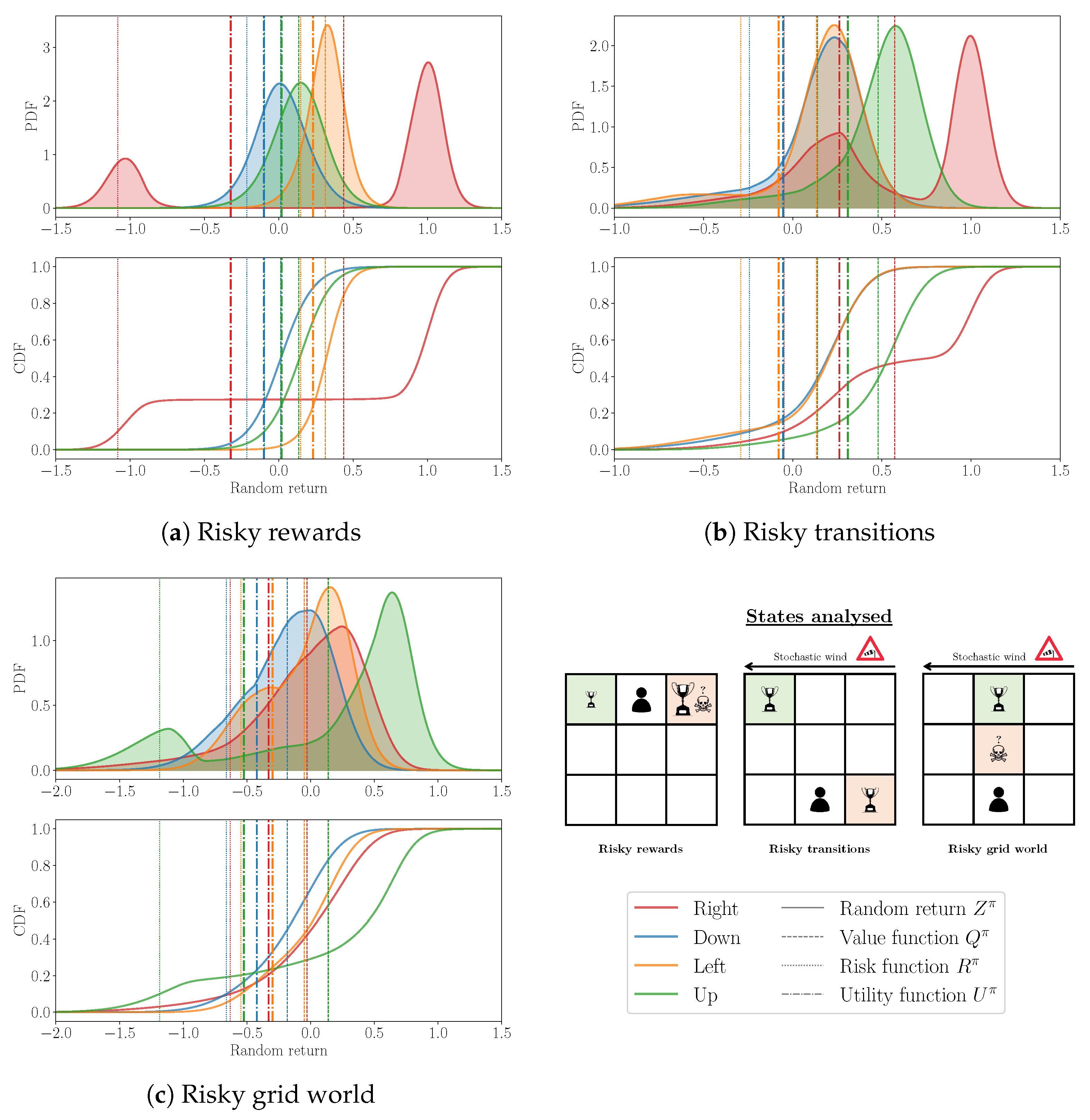
4.2. Probability Distribution Visualisation

A core advantage of the proposed solution is the improved interpretability of the resulting decision-making process. Indeed, the understanding and motivation of the decisions outputted by the learnt policy π is greatly facilitated by the access to the probability distributions of the random return jointly learnt. In addition, the analysis and comparison of the value, risk and utility functions ( Q π , R π and U π ) associated with different actions provide a valuable summary of the decision-making process, but also about the control problem itself. Such an analysis may be particularly important to correctly tune the risk trade-off parameter α according to the user’s risk aversion.
As an illustration, Figure 6 demonstrates some random return probability distributions Z π that are learnt by the RS-UMDQN-C algorithm. More precisely, a single relevant state is selected for analysis for each benchmark environment. The selection is based on the importance of the next decision in following a clear path, either maximising the expected outcome or mitigating the risk. Firstly, it can be observed that the risk-sensitive distributional RL algorithm manages to accurately learn the probability distributions of the random return, qualitatively, from a human perspective. In particular, the multimodality purposely designed to create risky situations appears to be well-preserved. Such a result is particularly encouraging, since this feature is essential to the success of the proposed methodology. Indeed, it ensures the accurate estimation of the risk, as defined in Section 3.2.2. This observation is in line with the findings of the research paper [27], introducing the UMDQN algorithm, and suggests that the solution introduced to achieve risk-sensitivity does not significantly alter the properties of the original distributional RL algorithm. Secondly, as previously explained, Figure 6 highlights the relevance of each function introduced ( Q π , R π and U π ) for making and motivating a decision. Their analysis truly contributes to the understanding of the potential trade-off between expected performance maximisation and risk mitigation for a given decision-making problem, as well as the extent to which different values of the important parameter α lead to divergent policies.

5. Conclusions

The present research work introduces a straightforward yet efficient solution to learning risk-sensitive decision-making policies based on the distributional RL approach. The proposed methodology presents key advantages. Firstly, it is perfectly compatible with any distributional RL algorithm, and requires only minimal modifications to the original algorithm. Secondly, the simplicity of the approach contributes to the interpretability and ease of analysis of the resulting risk-sensitive policies, a particularly important feature to avoid black-box machine learning models. Lastly, the solution can cover the complete potential trade-off between expected outcome maximisation and risk minimisation. The first experiments performed on three relevant toy problems yield promising results, which may be viewed as a proof of concept for the accessible and practical solution introduced.
Some interesting leads can be suggested as future work. Firstly, the research that was conducted is exclusively empirical and does not study any theoretical guarantees about the resulting risk-sensitive distributional RL algorithms. Among others, the study of the convergence of these algorithms would be a relevant future research direction. Secondly, building on the promising results achieved, the presented solution should definitely be evaluated on more complex environments, for which the risk should ideally be mitigated. Lastly, the approach could be extended to not only mitigate the risk but also to completely discard actions that would induce an excessive level of risk in order to increase compliance with the objective criterion originally defined in Section 3.2.1.

Author Contributions

Conceptualization, T.T.; Data curation, T.T.; Formal analysis, T.T.; Funding acquisition, T.T.; Investigation, T.T.; Methodology, T.T.; Project administration, D.E.; Resources, D.E.; Software, T.T.; Supervision, D.E.; Validation, D.E.; Visualization, T.T.; Writing—original draft, T.T.; Writing—review and editing, T.T. All authors have read and agreed to the published version of the manuscript.

Funding

Thibaut Théate is a Research Fellow of the F.R.S.-FNRS, of which he acknowledges the financial support.

Data Availability Statement

Not applicable.

Conflicts of Interest

The authors declare no conflict of interest.

Appendix A. Benchmark Environments

Risky rewards environment. The underlying MDP can be described as follows:
  • S { 0 , 1 , 2 } × { 0 , 1 , 2 } , a state s being composed of the two coordinates of the agent within the grid,
  • A = { RIGHT , DOWN , LEFT , UP } , with an action a being a moving direction,
  • p R ( r | s , a ) N ( μ , σ 2 ) where:
    μ = 0.3 and σ = 0.1 if the agent reaches the first objective location (terminal state),
    μ = 1.0 and σ = 0.1 with a 75% chance, and μ = 1.0 and σ = 0.1 with a 25% chance if the agent reaches the second objective location (terminal state),
    μ = 0.1 and σ = 0.1 otherwise,
  • p T ( s | s , a ) associates a 100% chance to move once in the chosen direction, while keeping the agent within the 3 × 3 grid world (crossing a border is not allowed),
  • p 0 associates a probability of 1 to the state s = [ 1 , 0 ] , which is the position of the agent in Figure 4,
  • γ = 0.9 .
Risky transitions environment. The underlying MDP can be described as the following:
  • S { 0 , 1 , 2 } × { 0 , 1 , 2 } , a state s being composed of the two coordinates of the agent within the grid,
  • A = { RIGHT , DOWN , LEFT , UP } , with an action a being a moving direction,
  • p R ( r | s , a ) N ( μ , σ 2 ) where:
    μ = 1.0 and σ = 0.1 if the agent reaches one of the objective locations (terminal state),
    μ = 0.3 and σ = 0.1 otherwise,
  • p T ( s | s , a ) associates a 100% chance to move once in the chosen direction AND a 50% chance to get pushed once to the left by the stochastic wind, while keeping the agent within the 3 × 3 grid world,
  • p 0 associates a probability of 1 to the state s = [ 1 , 0 ] , which is the position of the agent in Figure 4,
  • γ = 0.9 .
Risky grid world environment. The underlying MDP is described as follows:
  • S { 0 , 1 , 2 } × { 0 , 1 , 2 } , a state s being composed of the two coordinates of the agent within the grid,
  • A = { RIGHT , DOWN , LEFT , UP } , with an action a being a moving direction,
  • p R ( r | s , a ) N ( μ , σ 2 ) where:
    μ = 1.0 and σ = 0.1 if the agent reaches the objective location (terminal state),
    μ = 0.2 and σ = 0.1 with a 75% chance, and μ = 2.0 and σ = 0.1 with a 25% chance if the agent reaches the stochastic trap location (terminal state),
    μ = 0.2 and σ = 0.1 otherwise,
  • p T ( s | s , a ) associates a 100% chance to move once in the chosen direction AND a 25% chance to get pushed once to the left by the stochastic wind, while keeping the agent within the 3 × 3 grid world,
  • p 0 associates a probability of 1 to the state s = [ 1 , 0 ] , which is the position of the agent in Figure 4,
  • γ = 0.9 .

Appendix B. RS-UMDQN-C Algorithm

Algorithm A1 presents the novel Risk-Sensitive Unconstrained Monotonic Deep Q-Network with Cramer algorithm (RS-UMDQN-C). Basically, this new RL algorithm is the result of the application of the methodology described in Algorithm 1 to the UMDQN-C algorithm thoroughly introduced in [27].
Algorithm A1 RS-UMDQN-C algorithm
  • Initialise the experience replay memory M of capacity C.
  • Initialise the main UMNN weights θ (Xavier initialisation).
  • Initialise the target UMNN weights θ = θ .
  • for episode = 0 to N do
  •    for  t = 0 to T, or until episode termination do
  •       Acquire the state s from the environment E .
  •       With probability ϵ , select a random action a A .
  •       Otherwise, select a = argmax a A U ( s , a ; θ ) ,
  •       with U ( s , a ; θ ) = α E Z ( s , a ; θ ) + ( 1 α ) VaR ρ Z ( s , a ; θ ) .
  •       Interact with the environment E with action a to get the next state s and the reward r.
  •       Store the experience e = ( s , a , r , s ) in the experience replay memory M.
  •       Randomly sample from M a minibatch of N e experiences e i = ( s i , a i , r i , s i ) .
  •       Derive a discretisation of the domain X by sampling N z returns z U ( [ z min , z max ] ) .
  •       for  i = 0 to N e  do 
  •           for all  z X  do 
  •             if  s i is terminal then
  •                 Set y i ( z ) = 0 if z < r i , 1 otherwise .
  •             else
  •                 Set y i ( z ) = Z z r i γ | s i , argmax a i A U ( s i , a i ; θ ) ; θ .
  •             end if
  •           end for
  •       end for
  •       Compute the loss L C ( θ ) = i = 0 N e z X y i ( z ) Z ( z | s i , a i ; θ ) 2 1 / 2 .
  •       Clip the resulting gradient in the range [ 0 , 1 ] .
  •       Update the main UMNN parameters θ using the ADAM optimiser with learning rate L r .
  •       Update the target UMNN parameters θ = θ every N steps.
  •       Anneal the ϵ -greedy exploration parameter ϵ .
  •    end for
  • end for

References

  1. Sutton, R.S.; Barto, A.G. Reinforcement Learning: An Introduction; MIT Press: Cambridge, MA, USA, 2018. [Google Scholar]
  2. Watkins, C.J.C.H.; Dayan, P. Technical Note: Q-Learning. Mach. Learn. 1992, 8, 279–292. [Google Scholar] [CrossRef]
  3. Dulac-Arnold, G.; Levine, N.; Mankowitz, D.J.; Li, J.; Paduraru, C.; Gowal, S.; Hester, T. Challenges of real-world reinforcement learning: Definitions, benchmarks and analysis. Mach. Learn. 2021, 110, 2419–2468. [Google Scholar] [CrossRef]
  4. Gottesman, O.; Johansson, F.D.; Komorowski, M.; Faisal, A.A.; Sontag, D.; Doshi-Velez, F.; Celi, L.A. Guidelines for reinforcement learning in healthcare. Nat. Med. 2019, 25, 16–18. [Google Scholar] [CrossRef] [PubMed]
  5. Théate, T.; Ernst, D. An application of deep reinforcement learning to algorithmic trading. Expert Syst. Appl. 2021, 173, 114632. [Google Scholar] [CrossRef]
  6. Thananjeyan, B.; Balakrishna, A.; Nair, S.; Luo, M.; Srinivasan, K.; Hwang, M.; Gonzalez, J.E.; Ibarz, J.; Finn, C.; Goldberg, K. Recovery RL: Safe Reinforcement Learning with Learned Recovery Zones. IEEE Robot. Autom. Lett. 2021, 6, 4915–4922. [Google Scholar] [CrossRef]
  7. Zhu, Z.; Zhao, H. A Survey of Deep RL and IL for Autonomous Driving Policy Learning. IEEE Trans. Intell. Transp. Syst. 2022, 23, 14043–14065. [Google Scholar] [CrossRef]
  8. Bellemare, M.G.; Dabney, W.; Munos, R. A Distributional Perspective on Reinforcement Learning. In Proceedings of the 34th International Conference on Machine Learning, ICML 2017, Sydney, NSW, Australia, 6–11 August 2017; Volume 70, pp. 449–458. [Google Scholar]
  9. García, J.; Fernández, F. A comprehensive survey on safe reinforcement learning. J. Mach. Learn. Res. 2015, 16, 1437–1480. [Google Scholar]
  10. Castro, D.D.; Tamar, A.; Mannor, S. Policy Gradients with Variance Related Risk Criteria. In Proceedings of the 29th International Conference on Machine Learning, ICML 2012, Edinburgh, UK, 26 June–1 July 2012. [Google Scholar]
  11. La, P.; Ghavamzadeh, M. Actor-Critic Algorithms for Risk-Sensitive MDPs. In Proceedings of the Advances in Neural Information Processing Systems 26: 27th Annual Conference on Neural Information Processing Systems 2013, Lake Tahoe, NV, USA, 5–8 December 2013; pp. 252–260. [Google Scholar]
  12. Zhang, S.; Liu, B.; Whiteson, S. Mean-Variance Policy Iteration for Risk-Averse Reinforcement Learning. In Proceedings of the Thirty-Fifth AAAI Conference on Artificial Intelligence, AAAI 2021, Thirty-Third Conference on Innovative Applications of Artificial Intelligence, IAAI 2021, The Eleventh Symposium on Educational Advances in Artificial Intelligence, EAAI 2021, Virtual Event, 2–9 February 2021; AAAI Press: Washington, DC, USA, 2021; pp. 10905–10913. [Google Scholar]
  13. Rockafellar, R.T.; Uryasev, S. Conditional Value-at-Risk for General Loss Distributions. Corp. Financ. Organ. J. 2001, 7, 1443–1471. [Google Scholar] [CrossRef] [Green Version]
  14. Chow, Y.; Tamar, A.; Mannor, S.; Pavone, M. Risk-Sensitive and Robust Decision-Making: A CVaR Optimization Approach. In Proceedings of the Advances in Neural Information Processing Systems 28: Annual Conference on Neural Information Processing Systems 2015, Montreal, QC, Canada, 7–12 December 2015; pp. 1522–1530. [Google Scholar]
  15. Chow, Y.; Ghavamzadeh, M.; Janson, L.; Pavone, M. Risk-Constrained Reinforcement Learning with Percentile Risk Criteria. J. Mach. Learn. Res. 2017, 18, 167:1–167:51. [Google Scholar]
  16. Tamar, A.; Glassner, Y.; Mannor, S. Optimizing the CVaR via Sampling. In Proceedings of the Twenty-Ninth AAAI Conference on Artificial Intelligence, Austin, TX, USA, 25–30 January 2015; AAAI Press: Washington, DC, USA, 2015; pp. 2993–2999. [Google Scholar]
  17. Rajeswaran, A.; Ghotra, S.; Ravindran, B.; Levine, S. EPOpt: Learning Robust Neural Network Policies Using Model Ensembles. In Proceedings of the 5th International Conference on Learning Representations, ICLR 2017, Toulon, France, 24–26 April 2017. [Google Scholar]
  18. Hiraoka, T.; Imagawa, T.; Mori, T.; Onishi, T.; Tsuruoka, Y. Learning Robust Options by Conditional Value at Risk Optimization. In Proceedings of the Advances in Neural Information Processing Systems 32: Annual Conference on Neural Information Processing Systems 2019, NeurIPS 2019, Vancouver, BC, Canada, 8–14 December 2019; pp. 2615–2625. [Google Scholar]
  19. Shen, Y.; Tobia, M.J.; Sommer, T.; Obermayer, K. Risk-Sensitive Reinforcement Learning. Neural Comput. 2014, 26, 1298–1328. [Google Scholar] [CrossRef] [PubMed] [Green Version]
  20. Dabney, W.; Ostrovski, G.; Silver, D.; Munos, R. Implicit Quantile Networks for Distributional Reinforcement Learning. In Proceedings of the 35th International Conference on Machine Learning, ICML 2018, Stockholmsmässan, Stockholm, Sweden, 10–15 July 2018; Volume 80, pp. 1104–1113. [Google Scholar]
  21. Tang, Y.C.; Zhang, J.; Salakhutdinov, R. Worst Cases Policy Gradients. In Proceedings of the 3rd Annual Conference on Robot Learning, CoRL 2019, Osaka, Japan, 30 October–1 November 2019; Volume 100, pp. 1078–1093. [Google Scholar]
  22. Urpí, N.A.; Curi, S.; Krause, A. Risk-Averse Offline Reinforcement Learning. In Proceedings of the 9th International Conference on Learning Representations, ICLR 2021, Virtual Event, Austria, 3–7 May 2021. [Google Scholar]
  23. Yang, Q.; Simão, T.D.; Tindemans, S.; Spaan, M.T.J. Safety-constrained reinforcement learning with a distributional safety critic. Mach. Learn. 2022, 112, 859–887. [Google Scholar] [CrossRef]
  24. Pinto, L.; Davidson, J.; Sukthankar, R.; Gupta, A. Robust Adversarial Reinforcement Learning. In Proceedings of the 34th International Conference on Machine Learning, ICML 2017, Sydney, NSW, Australia, 6–11 August 2017; Volume 70, pp. 2817–2826. [Google Scholar]
  25. Qiu, W.; Wang, X.; Yu, R.; Wang, R.; He, X.; An, B.; Obraztsova, S.; Rabinovich, Z. RMIX: Learning Risk-Sensitive Policies for Cooperative Reinforcement Learning Agents. In Proceedings of the Advances in Neural Information Processing Systems 34: Annual Conference on Neural Information Processing Systems 2021, NeurIPS 2021, Virtual, 6–14 December 2021; pp. 23049–23062. [Google Scholar]
  26. Bellman, R. Dynamic Programming; Princeton University Press: Princeton, NJ, USA, 1957. [Google Scholar]
  27. Théate, T.; Wehenkel, A.; Bolland, A.; Louppe, G.; Ernst, D. Distributional Reinforcement Learning with Unconstrained Monotonic Neural Networks. Neurocomputing 2023, 534, 199–219. [Google Scholar] [CrossRef]
  28. Wehenkel, A.; Louppe, G. Unconstrained Monotonic Neural Networks. In Proceedings of the Advances in Neural Information Processing Systems 32: Annual Conference on Neural Information Processing Systems 2019, NeurIPS 2019, Vancouver, BC, Canada, 8–14 December 2019; pp. 1543–1553. [Google Scholar]
Figure 1. Intuitive graphical comparison between classical RL and distributional RL, for a decision-making policy π .
Algorithms 16 00325 g001
Figure 2. Illustration of the risk modelling adopted in this research work, based on the probability distribution of the random return Z π learnt by a distributional RL algorithm.
Algorithms 16 00325 g002
Figure 3. Illustration of the utility function U π for a typical random return probability distribution, with α = 0.75 in this case.
Algorithms 16 00325 g003
Figure 4. Illustration of the benchmark environments introduced in this research work for the performance assessment of risk-sensitive decision-making policies. The optimal objective locations/paths in terms of risk mitigation and expected return maximisation are highlighted in green and orange, respectively. (a) Risky rewards; (b) Risky transitions; (c) Risky grid world.
Algorithms 16 00325 g004
Figure 5. Evolution of the risk-sensitivity performance indicator R s (expected value of the random variable) achieved by the decision-making policies π learnt by both the DQN and RS-UMDQN-C algorithms during the training phase. (a) Risky rewards; (b) Risky transitions; (c) Risky grid world.
Algorithms 16 00325 g005
Figure 6. Visualisation of the random return probability distributions Z π learnt by the RS-UMDQN-C algorithm for typical states of the benchmark environments, together with the value, risk and utility functions that are derived ( Q π , R π and U π ). (a) Risky rewards; (b) Risky transitions; (c) Risky grid world.
Algorithms 16 00325 g006
Table 1. Description of the main hyperparameters used in the experiments.
HyperparameterSymbolValue
DNN structure- [ 128 , 128 ]
Learning rate L r 10 4
Deep learning optimiser epsilon- 10 5
Replay memory capacityC 10 4
Batch size N e 32
Target update frequency N 10 3
Random return resolution N z 200
Random return lower bound z min 2
Random return upper bound z max + 2
Exploration ϵ -greedy initial value- 1.0
Exploration ϵ -greedy final value- 0.01
Exploration ϵ -greedy decay- 10 4
Risk coefficient ρ 10 %
Risk trade-off α 0.5
Table 2. Comparison of the expectation E [ · ] , the risk function R ρ [ · ] and the utility function U [ · ] of the cumulative reward S π achieved by the decision-making policies π learnt by both the DQN and RS-UMDQN-C algorithms.
Benchmark EnvironmentDQNRS-UMDQN-C
E S π R ρ S π U S π E S π R ρ S π U S π
Risky rewards0.3−1.246−0.4740.1−0.126−0.013
Risky transitions0.7030.1180.4110.6250.3460.485
Risky grid world0.347−1.03−0.3420.3330.0180.175
Disclaimer/Publisher’s Note: The statements, opinions and data contained in all publications are solely those of the individual author(s) and contributor(s) and not of MDPI and/or the editor(s). MDPI and/or the editor(s) disclaim responsibility for any injury to people or property resulting from any ideas, methods, instructions or products referred to in the content.

