
The Extraction of Maximal-Sum Principal Submatrix and Its Applications


Abstract
1. Introduction
- (1)
- The integer programming models describing the two problems are different;
- (2)
- The formats of their solutions to the problems are different;
- (3)
- The purposes of the application problems are different.
2. Related Work
2.1. Best Submatrix Extraction
2.2. Color Combination Selection
2.3. Stock Investment Portfolio Construction
3. Problem Description and Related Property
3.1. Problem Description
3.2. MSPS Problem Optimization Model
3.3. Property
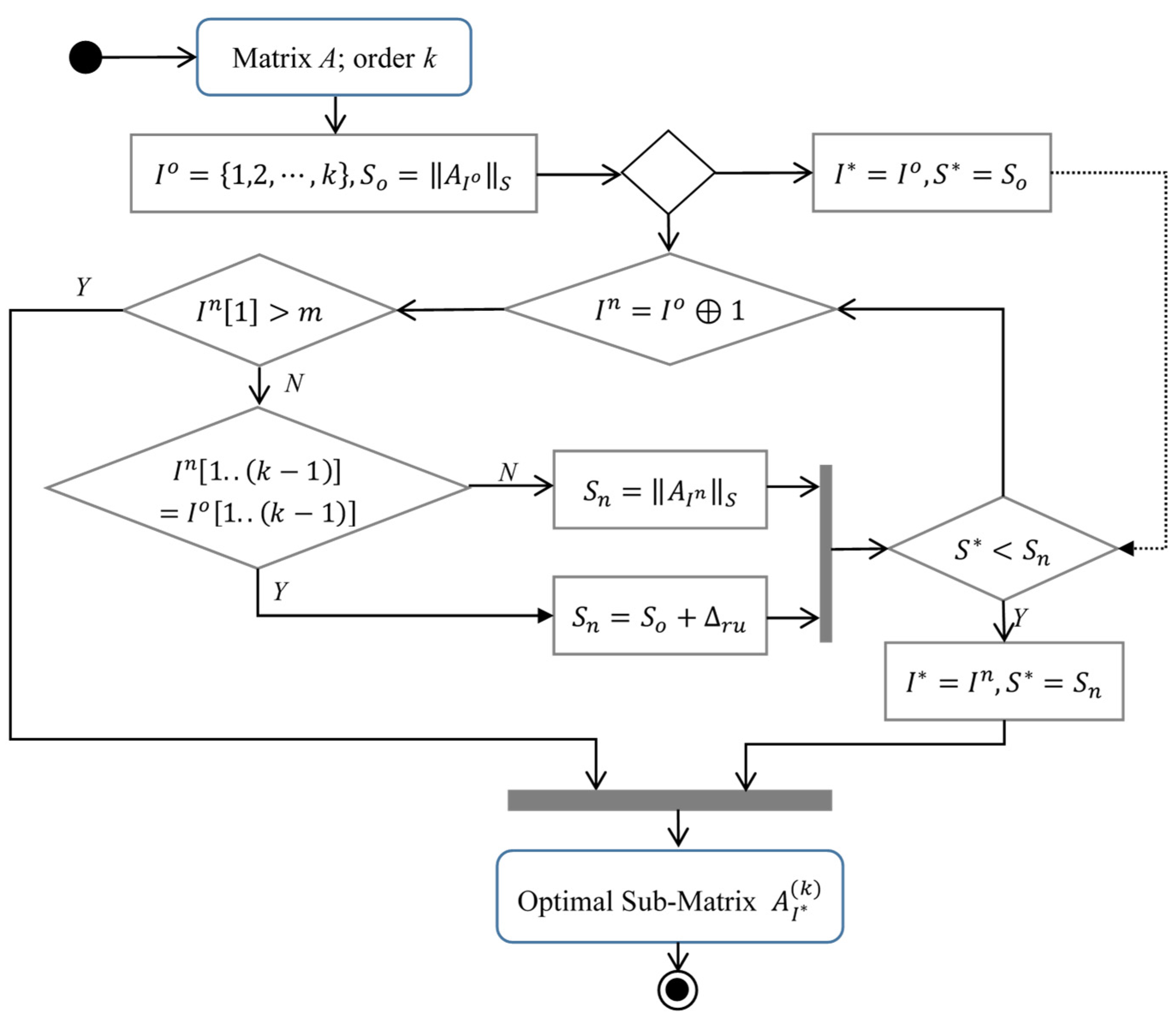
4. The Proposed Algorithm
| Algorithm 1: MSPS-RU algorithm |
| Input: A; //an -order real matrix ; //the order of the MSPS to be extracted Output: ; // the optimal index set of the MSPS 1 Let ; 2 build initial principal submatrix , ; 3 calculate the sum of all elements in , ; 4 while () 5 ;; 6 build next principal submatrix ; 7 if 8 ; // Formula (5) 9 else 10 ;// Formula (2) 11 endif 12 if 13 ; ; 14 endif 15 16 end while 17 return , ; |
5. Experiment
| Algorithm 2: Enum algorithm |
| Input: A; //an -order real matrix ; //the order of the MSPS to be extracted Output: ; // the optimal index set of the MSPS 1 Let ; 2 build initial principal submatrix , ; 3 calculate the sum of all elements in , ; 4 while () 5 ; ; 6 build next principal submatrix ; 7 ;// Formula (2) 8 if 9 ; ; 10 endif 11 12 end while 13 return , ; |
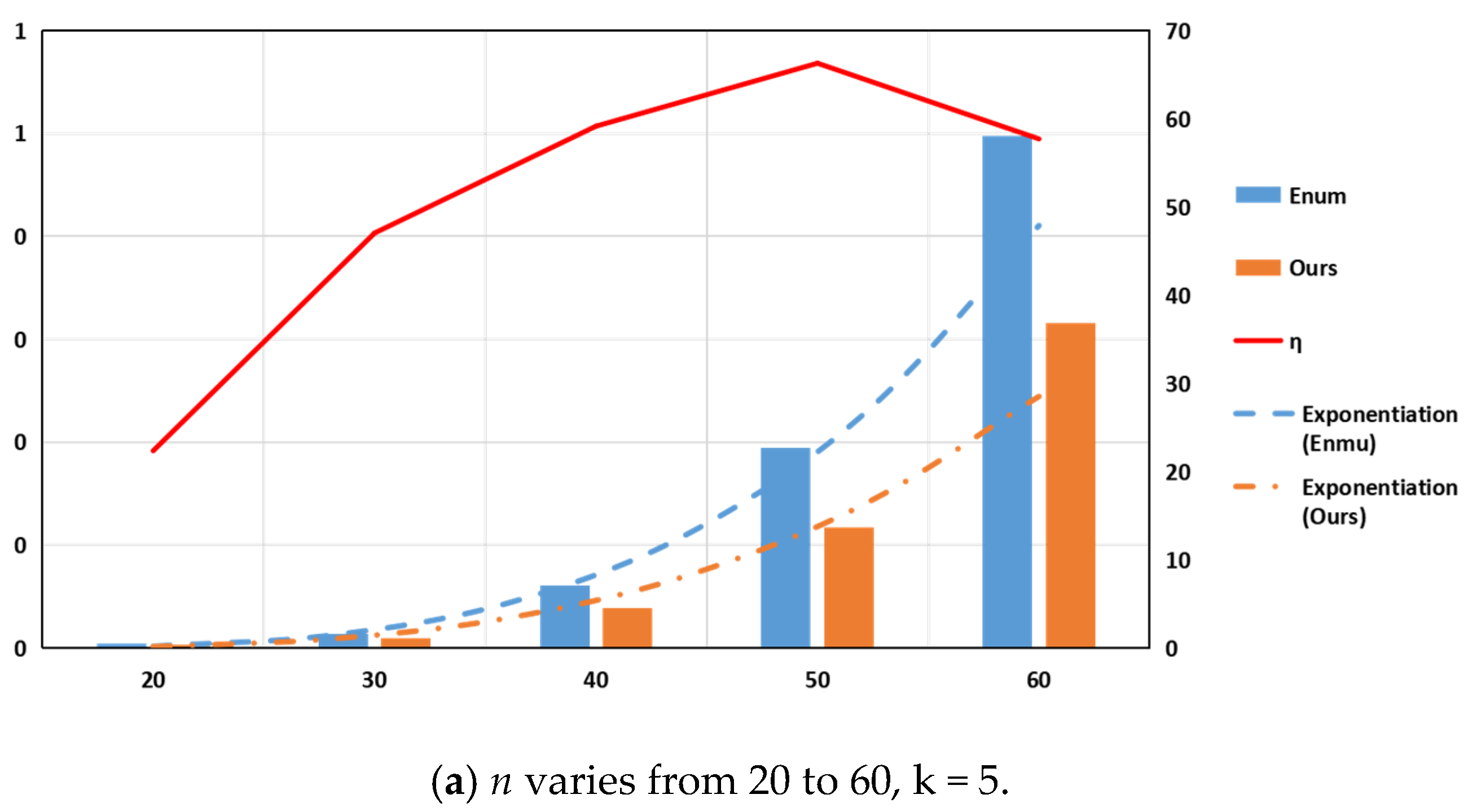
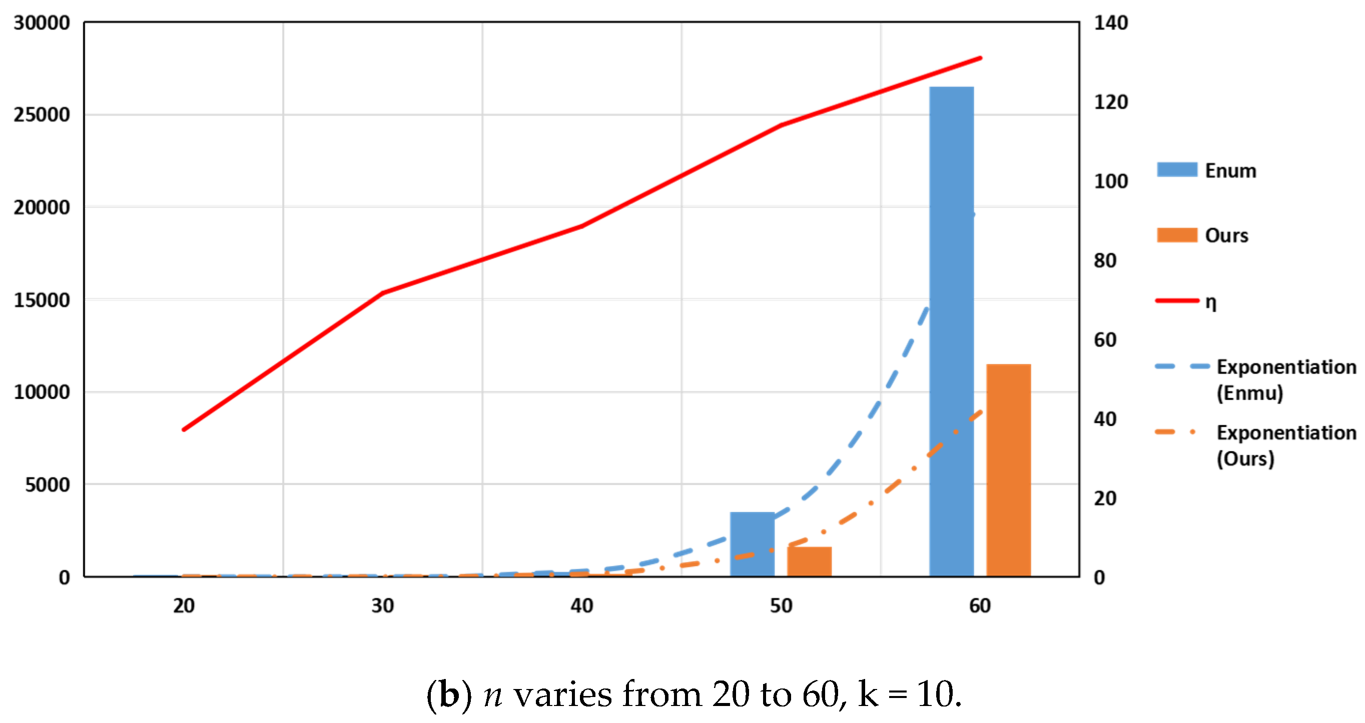
5.1. Parameter k Is Fixed and Parameter n Is Variable
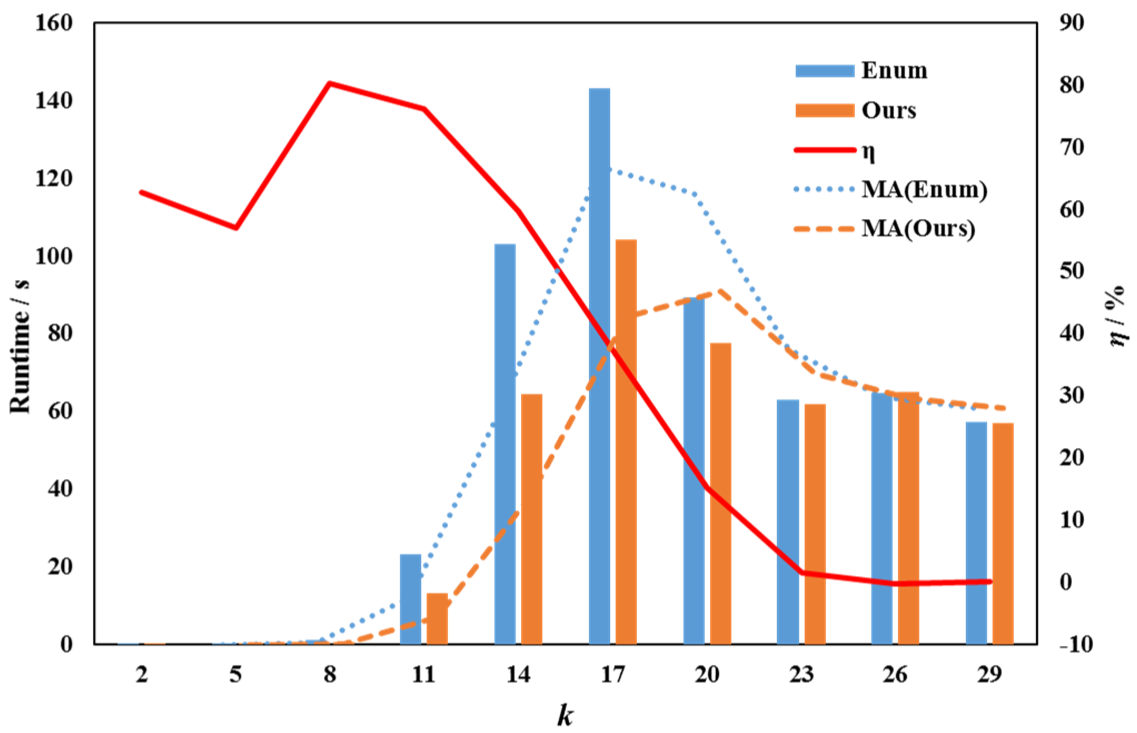
5.2. Parameter Is Fixed and Parameter Is Variable
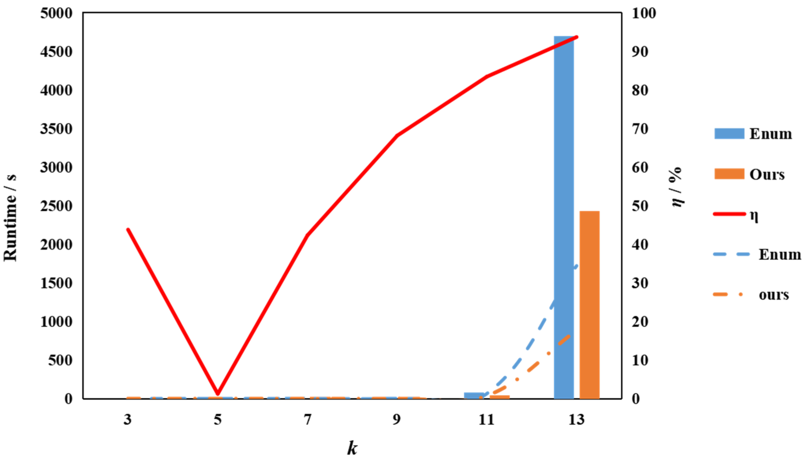
5.3. Parameters and Are Linear Function
6. Applications
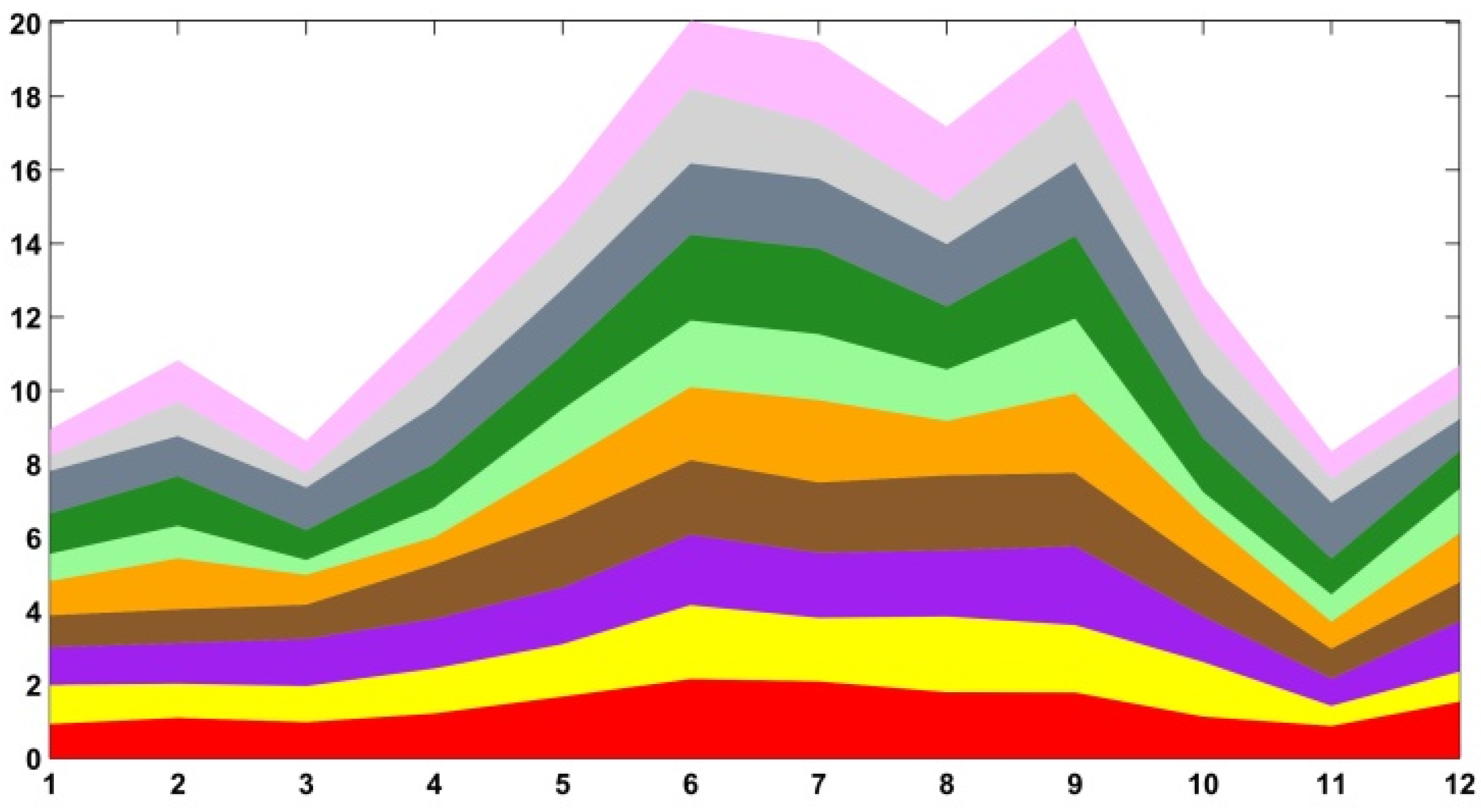
6.1. Construct a Optimal Color Combination
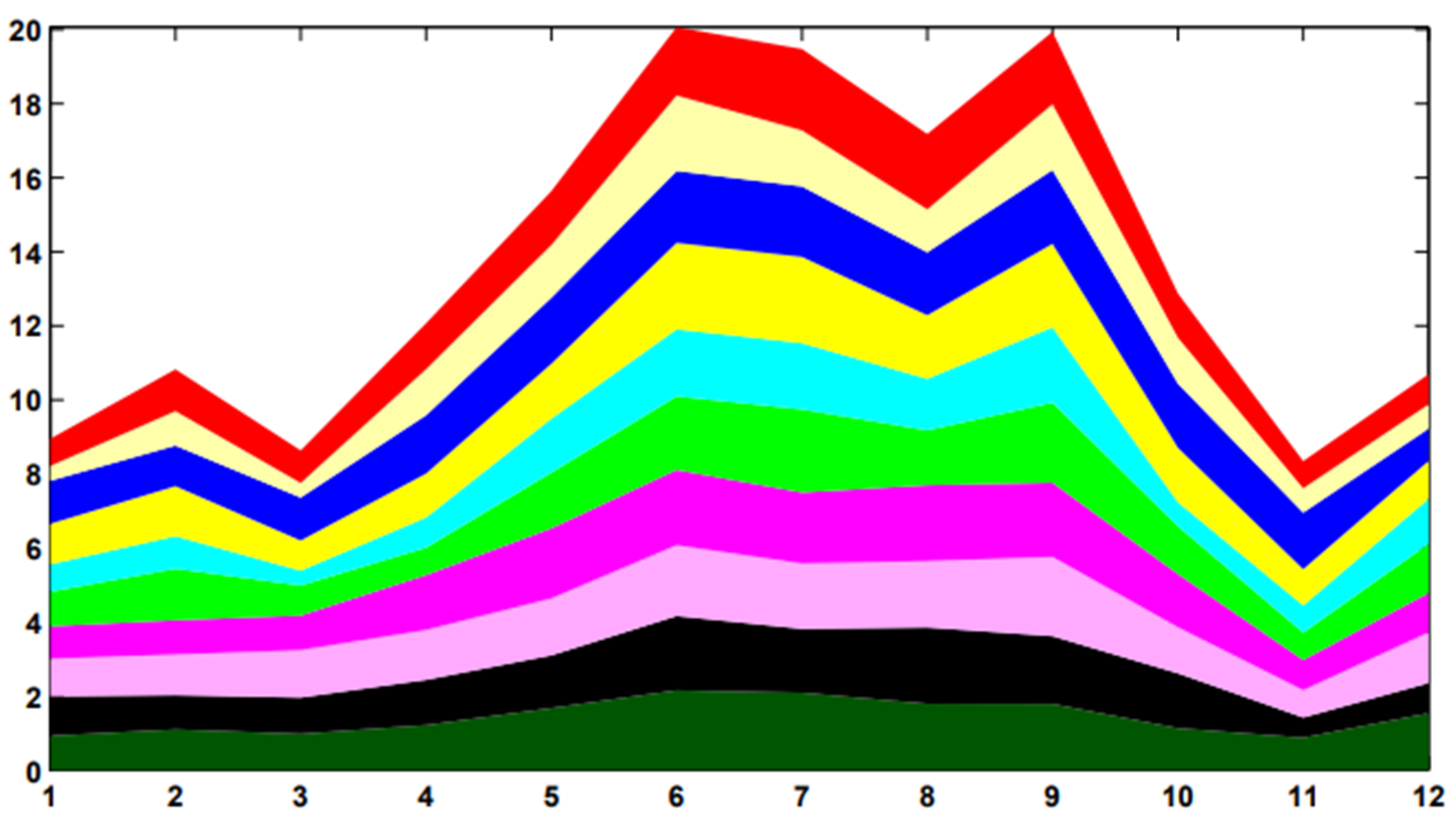
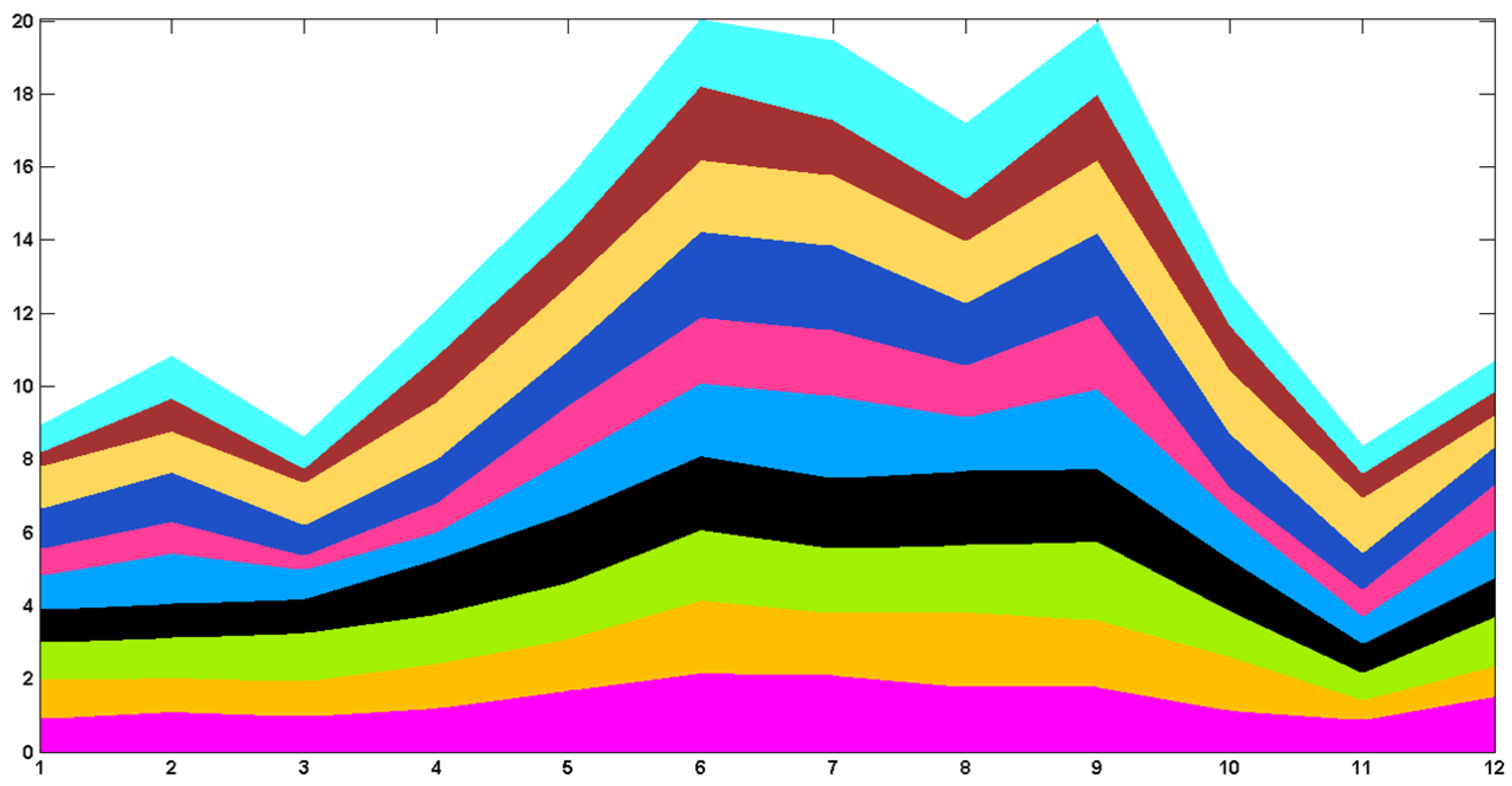
6.1.1. Construction of Color Distance Matrix
6.1.2. Application on Stacked Graph Coloring
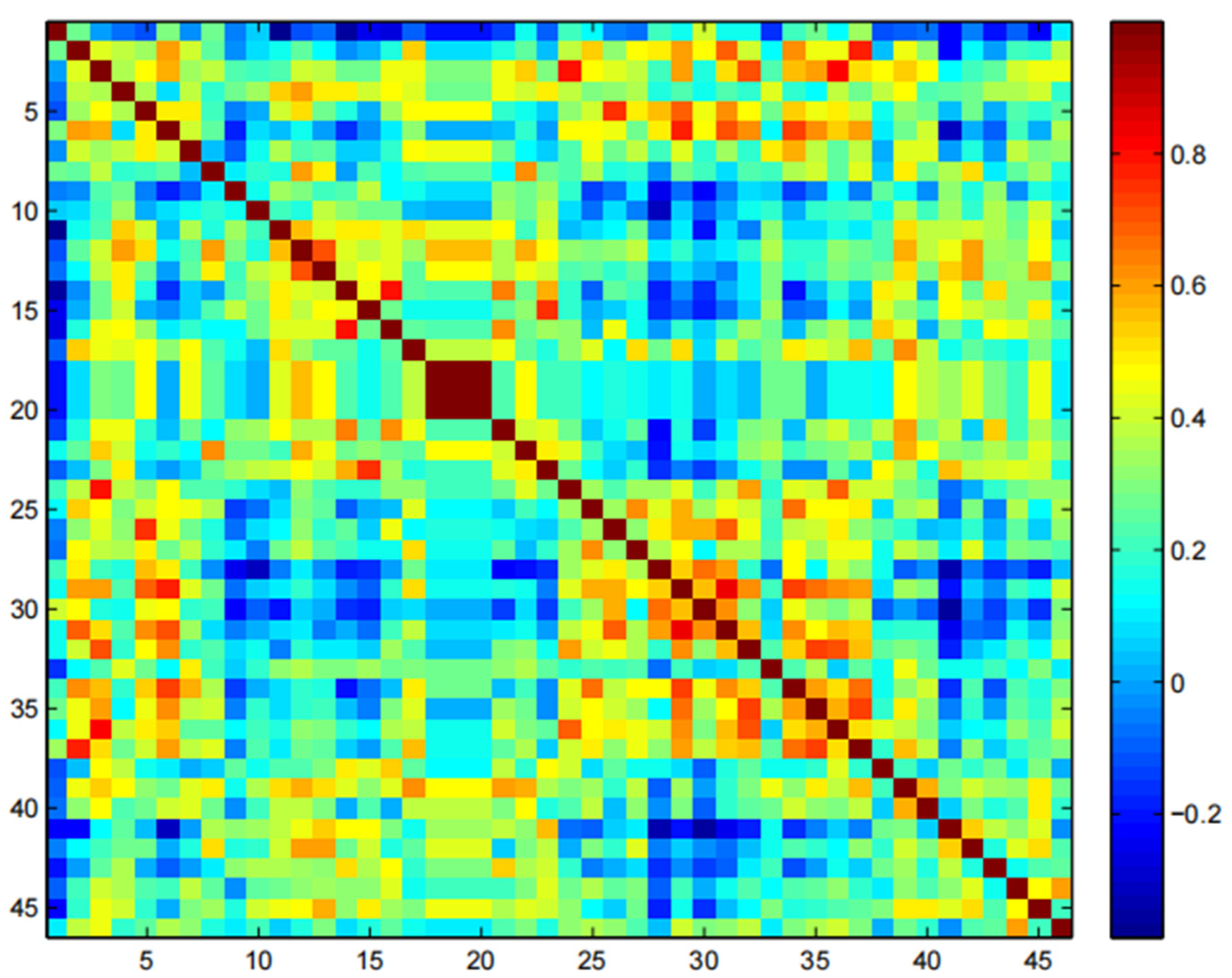
6.2. Construct a Optimal Stock Portfolio
- (1)
- Building a negative correlation coefficient matrix: Since MSPS-RU deals with the maximal problem, the minimum correlation degree can be converted to the maximal problem of the negative correlation coefficient matrix.
- (2)
- Using MSPS-RU algorithm to extract k stocks which have the maximal negative correlation degree.
- (3)
- Proposing investment suggestions.
| Algorithm 3: FP-MCD algorithm |
| Input: //The return rates of n candidate stocks in continuous t days; ; //the number of stocks in the portfolio ; // days used for learning, constructing the correlation coefficient matrix; days used to test portfolio returns Output: ; // the optimal index set of the n candidate stocks 1 Let ; 2 Construct the correlation coefficient matrix using ; 3 Build the negative correlation coefficient matrix ; 4 Use MSPS-RU to obtain the optimal portfolio 5 Test portfolio returns with and data ; 6 If the is accepted 7 return ; 8 else 9 return ; 10 endif |
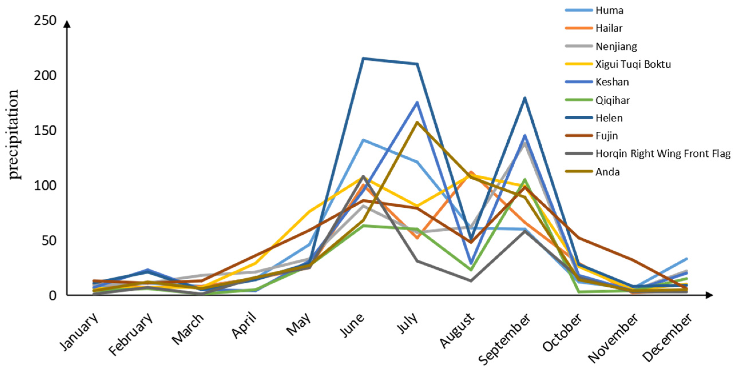
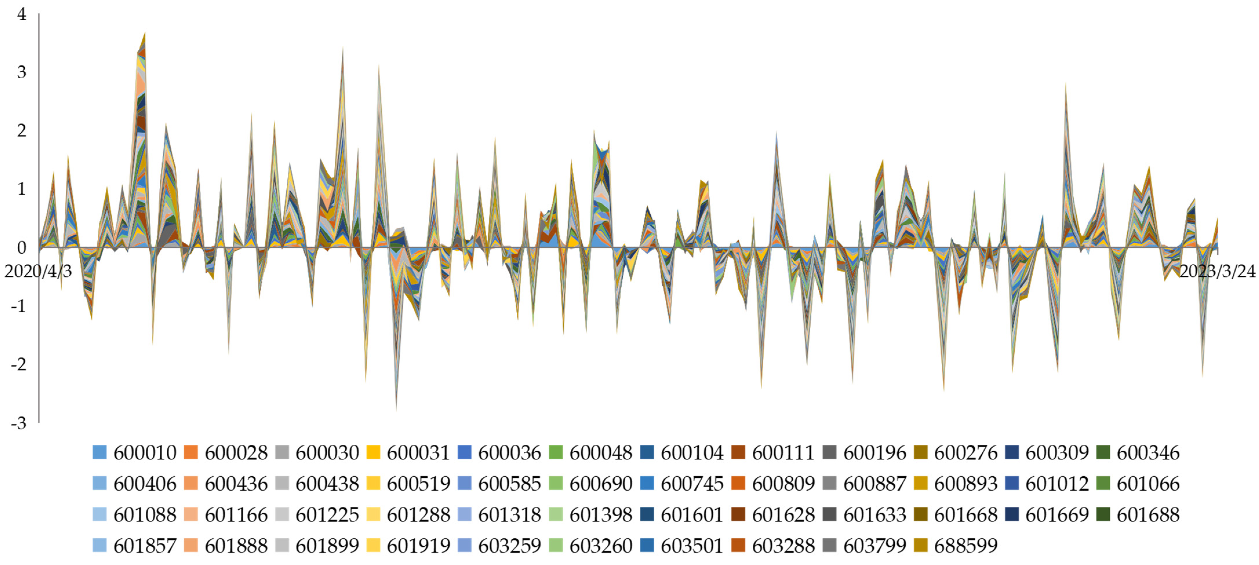
6.2.1. Data
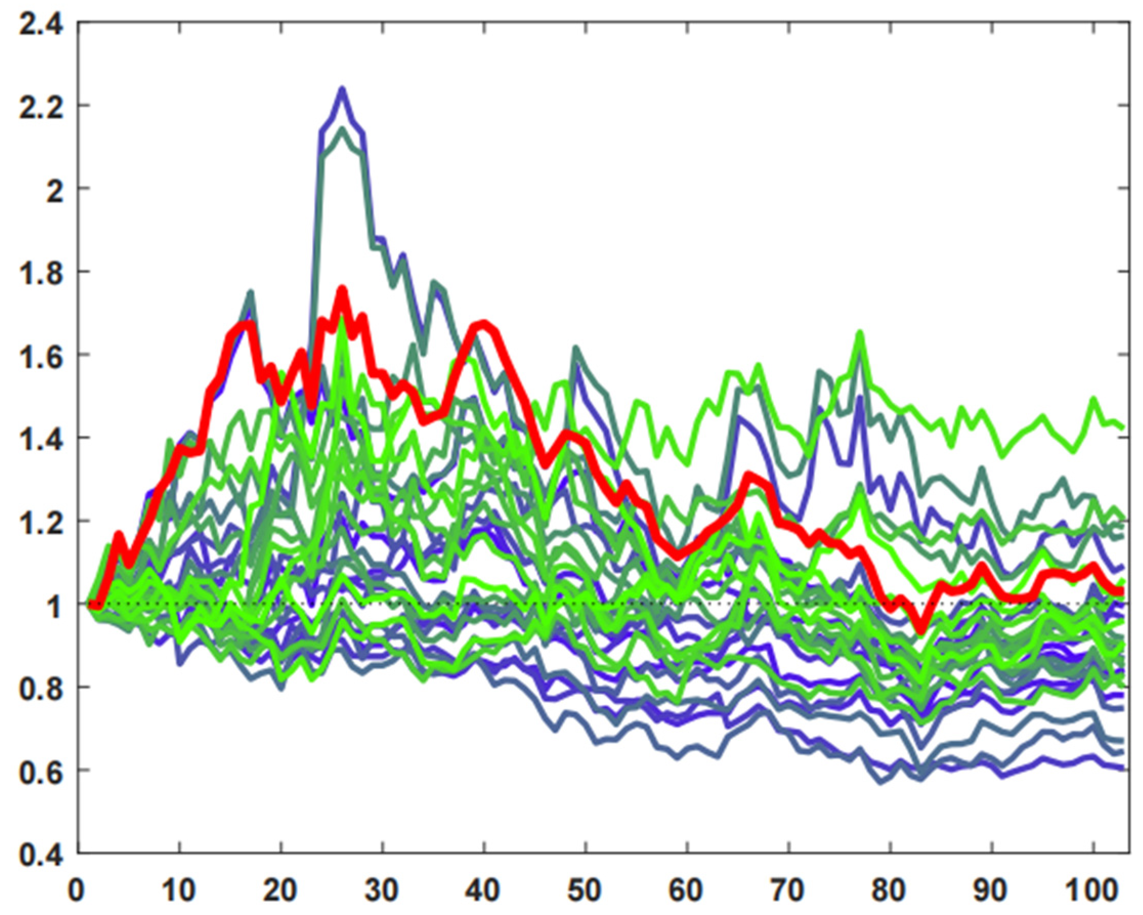
6.2.2. Construct the Optimal Investment Portfolio
6.2.3. Test the Optimal Investment Portfolio
7. Conclusions
Author Contributions
Funding
Data Availability Statement
Acknowledgments
Conflicts of Interest
References
- Branders, V.; Schaus, P.; Dupont, P. Combinatorial optimization algorithms to mine a sub-matrix of maximal sum. In Proceedings of the 6th International Workshop on New Frontiers in Mining Complex Patterns in Conjunction with ECML-PKDD 2017, Skopje, Macedonia, 18–22 September 2017; Lecture Notes in Computer Science. Springer International Publishing: Berlin/Heidelberg, Germany, 2018; Volume 10785, pp. 65–79. [Google Scholar] [CrossRef]
- Derval, G.; Schaus, P. Maximal-Sum submatrix search using a hybrid contraint programming/linear programming approach. Eur. J. Oper. Res. 2022, 297, 853–865. [Google Scholar] [CrossRef]
- Ferreira, C.S.; Camargo, R.Y.; Song, S.W. A Parallel Maximum Subarray Algorithm on GPUs. In Proceedings of the 2014 International Symposium on Computer Architecture and High Performance Computing Workshop, Paris, France, 22–24 October 2014; pp. 12–17. [Google Scholar] [CrossRef]
- Weddell, S.J.; Read, T.R.; Thaher, M.; Takaoka, T. Maximum subarray algorithms for use in astronomical imaging. J. Electron. Imaging 2013, 22, 043011. [Google Scholar] [CrossRef]
- Koch, I.; Marenco, J. The maximum 2D subarray polytope: Facet-inducing inequalities and polyhedral computations. Discret. Appl. Math. 2022, 323, 286–301. [Google Scholar] [CrossRef]
- Li, Y.; Xie, W. Best Principal Submatrix Selection for the Maximum Entropy Sampling Problem: Scalable Algorithms and Performance Guarantees. arXiv 2023, arXiv:2001.08537. [Google Scholar] [CrossRef]
- Macambira, E.M. An Application of Tabu Search Heuristic for the Maximum Edge-Weighted Subgraph Problem. Ann. Oper. Res. 2002, 117, 175–190. [Google Scholar] [CrossRef]
- Massei, S. Some algorithms for maximum volume and cross approximation of symmetric semidefinite matrices. BIT Numer. Math. 2022, 62, 195–220. [Google Scholar] [CrossRef]
- Lewis, S.C. On the Best Principal Submatrix Problem. Ph.D. Thesis, University of Birmingham, Birmingham, UK, 2006. [Google Scholar]
- Wen, Z. Fast parallel algorithms for the maximum sum problem. Parallel Comput. 1995, 21, 461–466. [Google Scholar] [CrossRef]
- Tamaki, H.; Tokuyama, T. Algorithms for the Maximum Subarray Problem Based on Matrix Multiplication. Interdiscip. Inf. Sci. 2000, 6, 99–104. [Google Scholar] [CrossRef]
- Takaoka, T. Efficient Algorithms for the Maximum Subarray Problem by Distance Matrix Multiplication. Electron. Notes Theor. Comput. Sci. 2002, 61, 191–200. [Google Scholar] [CrossRef]
- He, Y.; Li, H. Optimal layout of stacked graph for visualizing multidimensional financial timeseries data. Inf. Vis. 2022, 21, 63–73. [Google Scholar] [CrossRef]
- Healey, C.G. Choosing effective colours for data visualization. In Proceedings of the Seventh Annual IEEE Visualization ’96, San Francisco, CA, USA, 27 October–1 November 1996; pp. 263–270. [Google Scholar] [CrossRef]
- Zhou, L.; Hansen, C.D. A Survey of Colormaps in Visualization. IEEE Trans. Vis. Comput. Graph. 2016, 22, 2051–2069. [Google Scholar] [CrossRef] [PubMed]
- El-Assady, M.; Kehlbeck, R.; Metz, Y.; Schlegel, U.; Sevastjanova, R.; Sperrle, F.; Spinner, T. Semantic Color Mapping: A Pipeline for Assigning Meaningful Colors to Text. In Proceedings of the 2022 IEEE 4th Workshop on Visualization Guidelines in Research, Design, and Education (VisGuides), Oklahoma City, OK, USA, 17 October 2022; pp. 16–22. [Google Scholar]
- Anderson, C.L.; Robinson, A.C. Affective Congruence in Visualization Design: Influences on Reading Categorical Maps. IEEE Trans. Vis. Comput. Graph. 2022, 28, 2867–2878. [Google Scholar] [CrossRef] [PubMed]
- Samsel, F.; Bartram, L.; Bares, A. Art, Affect and Color: Creating Engaging Expressive Scientific Visualization. In Proceedings of the IEEE VISAP, Berlin, Germany, 23–26 October 2018. [Google Scholar]
- Wang, Y.; Chen, X.; Ge, T.; Bao, C.; Sedlmair, M.; Fu, C.-W.; Deussen, O.; Chen, B. Optimizing Color Assignment for Perception of Class Separability in Multiclass Scatterplots. IEEE Trans. Vis. Comput. Graph. 2019, 25, 820–829. [Google Scholar] [CrossRef] [PubMed]
- Abeyta, R.N. The Distance between Colors; Using DeltaE* to Determine Which Colors Are Compatible. Ph.D. Thesis, Embry-Riddle Aeronautical University, Daytona Beach, FL, USA, 2011. Available online: https://commons.erau.edu/edt/9 (accessed on 23 June 2023).
- Ledoit, O.; Wolf, M. Improved estimation of the covariance matrix of stock returns with an application to portfolio selection. J. Empir. Financ. 2003, 10, 603–621. [Google Scholar] [CrossRef]
- Onali, E.; Mascia, D.V. Corporate diversification and stock risk: Evidence from a global shock Author links open overlay panel. J. Corp. Financ. 2022, 72, 102150. [Google Scholar] [CrossRef]
- Markowitz, H. Portfolio selection. J. Financ. 1952, 7, 77–91. [Google Scholar]
- Ruppert, D.; Matteson, D.S. Portfolio Selection. In Springer Texts in Statistics; Springer: Berlin/Heidelberg, Germany, 2015; pp. 465–493. [Google Scholar] [CrossRef]
- Tiwari, A.K.; Abakah, E.J.A.; Karikari, N.K.; Hammoudeh, S. Time-varying dependence dynamics between international commodity prices and Australian industry stock returns: A Perspective for portfolio diversification. Energy Econ. 2022, 108, 105891. [Google Scholar] [CrossRef]
- Institute of Geographic Sciences and Resources, Chinese Academy of Sciences. Monthly Precipitation over the Years (by Station), Dataset. Available online: http://www.data.ac.cn/table/tbc40 (accessed on 21 May 2023).
- Moledina, A.A.; Roe, T.L.; Shane, M. Measuring commodity price volatility and the welfare consequences of eliminating volatility. In Proceedings of the American Agricultural Economics Association Annual Meeting, Denver, CO, USA, 1–4 August 2004; 25p. [Google Scholar]


| Ref. | Object | Connectivity | Principal Submatrix or Not | Submatrix Order | Accurate or Approximate Solution |
|---|---|---|---|---|---|
| [1] | The sum of the entries of submatrix | Discrete | N | Unfixed | Accurate |
| [2] | The sum of the entries of submatrix | Discrete | N | Unfixed | Approximate |
| [3,4,5] | The sum of the entries of submatrix | Consecutive | N | Unfixed | Accurate |
| [6] | The determinant of submatrix + | Discrete | Y | Fixed | Approximate |
| [7] | The sum of the entries of submatrix ++ | Discrete | Y | Fixed | Approximate |
| [8] | The maximum volume submatrix | Discrete | Y | Fixed | Approximate |
| Ours | The sum of the entries of submatrix | Discrete | Y | Fixed | Accurate |
| n | k | (%) | k | (%) | ||||
|---|---|---|---|---|---|---|---|---|
| 20 | 5 | 0.0020 | 0.0016 | 22.36 | 10 | 0.0746 | 0.0544 | 37.15 |
| 30 | 5 | 0.0138 | 0.0094 | 47.04 | 10 | 10.5342 | 6.1387 | 71.60 |
| 40 | 5 | 0.0610 | 0.0384 | 59.15 | 10 | 289.4542 | 153.5836 | 88.47 |
| 50 | 5 | 0.1946 | 0.1170 | 66.29 | 10 | 3485.9831 | 1629.6164 | 113.91 |
| 60 | 5 | 0.4980 | 0.3157 | 57.71 | 10 | 26,507.8060 | 11,480.9314 | 130.89 |
| k | TEnum | Tours | η (%) |
|---|---|---|---|
| 2 | 0.0015 | 0.0009 | 62.76 |
| 5 | 0.0155 | 0.0099 | 57.02 |
| 8 | 1.3105 | 0.7269 | 80.29 |
| 11 | 23.2704 | 13.2104 | 76.15 |
| 14 | 102.9598 | 64.4397 | 59.78 |
| 17 | 143.0534 | 104.1774 | 37.32 |
| 20 | 89.3660 | 77.5431 | 15.25 |
| 23 | 62.8989 | 61.8635 | 1.67 |
| 26 | 64.7635 | 64.9295 | −0.26 |
| 29 | 57.2279 | 57.1216 | 0.19 |
| n | k | |||
|---|---|---|---|---|
| 9 | 3 | 0.001115 | 0.000776 | 43.76 |
| 15 | 5 | 0.000785 | 0.000775 | 1.23 |
| 21 | 7 | 0.022176 | 0.015587 | 42.27 |
| 27 | 9 | 1.362391 | 0.810531 | 68.09 |
| 33 | 11 | 81.17768 | 44.27129 | 83.36 |
| 39 | 13 | 4693.559 | 2424.06 | 93.62 |
| k | Portfolios |
|---|---|
| 3 | 1 14 40 |
| 4 | 1 14 28 41 |
| 5 | 1 9 14 28 40 |
| 6 | 1 9 16 28 40 41 |
| 7 | 1 9 14 28 30 40 41 |
| 8 | 1 9 14 28 30 33 40 41 |
| 9 | 1 9 14 28 30 33 40 41 44 |
| 10 | 1 9 10 28 30 33 38 40 41 44 |
| Indicator | Ours | Rnd1 | Rnd2 | Rnd3 | Rnd4 | Rnd5 | Rnd6 | Rnd7 | Rnd8 | Rnd9 | Rnd10 |
| 0.0278 | 0.0307 | 0.0260 | 0.0133 | 0.0197 | 0.0343 | 0.0172 | 0.0291 | 0.0293 | 0.0220 | 0.0316 | |
| Ret | 1.0332 | 1.0197 | 1.0300 | 0.9862 | 0.9584 | 1.0240 | 1.0260 | 1.0024 | 1.0029 | 1.0522 | 0.9509 |
| Indicator | Rnd11 | Rnd12 | Rnd13 | Rnd14 | Rnd15 | Rnd16 | Rnd17 | Rnd18 | Rnd19 | Rnd20 | |
| 0.0243 | 0.0229 | 0.0289 | 0.0189 | 0.0251 | 0.0149 | 0.0312 | 0.0302 | 0.0237 | 0.0135 | ||
| Ret | 0.9866 | 1.0366 | 1.0564 | 1.0164 | 1.0185 | 1.0353 | 1.0451 | 0.9961 | 0.9950 | 1.0168 | |
| Indicator | Rnd21 | Rnd22 | Rnd23 | Rnd24 | Rnd25 | Rnd26 | Rnd27 | Rnd28 | Rnd29 | Rnd30 | |
| 0.0260 | 0.0206 | 0.0410 | 0.0287 | 0.0250 | 0.0242 | 0.0206 | 0.0264 | 0.0204 | 0.0169 | ||
| Ret | 1.0243 | 1.0055 | 1.0170 | 1.0244 | 1.0165 | 1.0361 | 1.0388 | 1.0386 | 1.0122 | 0.9902 |
| Diff. | Rnd1 | Rnd2 | Rnd3 | Rnd4 | Rnd5 | Rnd6 | Rnd7 | Rnd8 | Rnd9 | Rnd10 |
| 0.0028 | −0.0019 | −0.0146 | −0.0081 | 0.0064 | −0.0106 | 0.0013 | 0.0015 | −0.0058 | 0.0038 | |
| Ret | −0.0134 | −0.0031 | −0.0470 | −0.0747 | −0.0092 | −0.0072 | −0.0308 | −0.0302 | −0.0190 | −0.0823 |
| Diff. | Rnd11 | Rnd12 | Rnd13 | Rnd14 | Rnd15 | Rnd16 | Rnd17 | Rnd18 | Rnd19 | Rnd20 |
| −0.0035 | −0.0049 | 0.0011 | −0.0089 | −0.0028 | −0.0129 | 0.0034 | 0.0023 | −0.0042 | −0.0143 | |
| Ret | −0.0466 | 0.0034 | 0.0232 | −0.0167 | −0.0146 | 0.00215 | 0.0119 | −0.0371 | −0.0382 | −0.0163 |
| Diff. | Rnd21 | Rnd22 | Rnd23 | Rnd24 | Rnd25 | Rnd26 | Rnd27 | Rnd28 | Rnd29 | Rnd30 |
| −0.0018 | −0.0073 | 0.0132 | 0.0008 | −0.0028 | −0.0036 | −0.0072 | −0.0015 | −0.0074 | −0.0109 | |
| Ret | −0.0089 | −0.0277 | −0.0162 | −0.0088 | −0.0167 | 0.0029 | 0.0057 | 0.0055 | −0.0210 | −0.0430 |
Disclaimer/Publisher’s Note: The statements, opinions and data contained in all publications are solely those of the individual author(s) and contributor(s) and not of MDPI and/or the editor(s). MDPI and/or the editor(s) disclaim responsibility for any injury to people or property resulting from any ideas, methods, instructions or products referred to in the content. |
© 2023 by the authors. Licensee MDPI, Basel, Switzerland. This article is an open access article distributed under the terms and conditions of the Creative Commons Attribution (CC BY) license (https://creativecommons.org/licenses/by/4.0/).
Share and Cite
Zhang, Y.; Luo, L.; Li, H. The Extraction of Maximal-Sum Principal Submatrix and Its Applications. Algorithms 2023, 16, 314. https://doi.org/10.3390/a16070314
Zhang Y, Luo L, Li H. The Extraction of Maximal-Sum Principal Submatrix and Its Applications. Algorithms. 2023; 16(7):314. https://doi.org/10.3390/a16070314
Chicago/Turabian StyleZhang, Yizheng, Liuhong Luo, and Hongjun Li. 2023. "The Extraction of Maximal-Sum Principal Submatrix and Its Applications" Algorithms 16, no. 7: 314. https://doi.org/10.3390/a16070314
APA StyleZhang, Y., Luo, L., & Li, H. (2023). The Extraction of Maximal-Sum Principal Submatrix and Its Applications. Algorithms, 16(7), 314. https://doi.org/10.3390/a16070314