1. Introduction
Autism spectrum disorder (ASD) is a generalized neurodevelopmental disorder characterized by difficulty in social communication, repetitive patterns of behavior, and narrow interests [
1]. Recent studies show that 23 out of every 1000 eight-year-olds in the United States have ASD [
2]. Early diagnosis and intervention are key to preventing the exacerbation of symptoms in ASD patients, improving the quality of life of patients and easing the burden on families [
3]. At present, the diagnosis of autism is based on symptom-based clinical criteria, which requires a large number of behavioral assessments and requires high professional knowledge of doctors. Moreover, the diagnosis results are affected by doctors’ subjectivity, which may lead to misdiagnosis and delayed diagnosis [
4]. Therefore, it is necessary to develop an objective, accurate and rapid diagnostic method for ASD. Neuroimaging has been shown to be useful in diagnosing brain diseases and explaining underlying pathologic mechanisms [
5]. Resting-state functional magnetic resonance imaging (rs-fMRI) has become one of the commonly used imaging methods in ASD research due to its non-invasiveness, easy acquisition, low patient effort and high generalization ability [
6,
7,
8].
The amount of rs-fMRI data at a single site is usually small, leading to the possibility of disputable reproducibility and universality of studies [
9]; using multi-site data to compose big data integration is an effective method to solve this problem. Autism Brain Imaging Data Exchange (ABIDE) aggregates functional and structural brain imaging collected by laboratories around the world, providing a public multi-site dataset for ASD-related research. In specific ASD classification methods, the high dimension of the original image may lead to model overfitting, and the derived functional connectivity dimension is low and can reflect the specific characteristics of ASD [
10], so most methods detect autism spectrum disorders from functional connectivity. For example, Eslami et al. [
11] designed a joint learning program of autoencoder (AE) and single-layer perceptrons, connected these networks with low-dimension representations in a mixed way with learning functions, and completed classification on ABIDE multi-site data to reach an accuracy of 70.3%. Wang et al. [
12] first defined the graph structure based on functional connections, and proposed a graph convolutional network (cGCN) based on functional connections for ASD classification. This method can extract the spatial features of the neighbor domain of the target brain region from the functional connections. The neighbors of the target brain area are calculated by group functional connections, and each convolution result is the feature of the target brain area. Therefore, the feature finally extracted is the result of all brain areas after considering the functional neighbor information, which can be consistent with the functional organization of the brain. The purpose of the design is to make the convolution operation have brain physiological significance, so as to extract features more efficiently. Finally, the accuracy rate reaches 71.6%.
However, different sites usually have differences in collection equipment, collection parameters and collection population, which results in the natural heterogeneity of multi-site datasets [
9,
13]. The confounding effect caused by multiple sites will affect the relationship between input data and output variables, leading to the correlation between site differences and biological predictions. Such correlations can hamper estimates of true biological changes, or extrapolate non-biological differences to biological differences, resulting in false or biased predictions from models [
14]. For example, when the collection equipment is different, the fMRI images obtained by the same subject will be different, which will affect the analysis of physiological differences such as gender differences [
15]. For example, when the purpose of a neuroimaging study is to distinguish between healthy individuals and patients with ASD, if the number of patients at one site is significantly higher than that at another site, the characteristics of the differences in the data at that site may be the criteria for the model to identify the disease. This heterogeneity has the result that although many methods can obtain relatively high accuracy at a single site, when applied to datasets at other sites, the trained models usually fail to achieve an acceptable performance [
16,
17], which is not conducive to early intervention and auxiliary diagnosis of ASD. For example, Nielsen et al. [
16] achieve a maximum classification accuracy of 90% in the single-site ASD classification experiment of ABIDE dataset, but only a maximum classification accuracy of 60% in the multi-site ASD classification experiment of 17 sites.
There are two methods to solve multi-site data heterogeneity: data processing and model-based. The method based on data processing solves the problem of multiple sites by eliminating the difference of data domain distribution between sites. For example, Wang et al. [
18] proposed a multi-site adaptive framework based on low-rank representation decomposition, in which the data of one site are regarded as the target domain and the data of other sites as the source domain, and the data in these domains are converted into a low-rank representation public space, so as to reduce the difference in data distribution among different sites. Model-based studies remove the influence of sites through the model itself. For example, Dinsdale et al. [
19] proposed a training scheme based on deep learning, which uses iterative updating to remove scanner information and generate unchanged shared features of sites, so as to realize the prediction of a site-free model. In addition, in the study on removing the influence of confounding effects, Zhao et al. [
20] proposed an end-to-end method, which quantifies the statistical dependence between the features extracted from the model and confounding factors, so as to guide the elimination of confounding effects in the process of feature extraction. The experimental results show that the model has a high accuracy in AIDS classification after removing confounding factors.
In the above methods to solve the multi-site problem, the site data domain mapping and classifier training based on data processing are independent of each other, which may reduce the learning performance, so it is necessary to design a new framework to make the two interrelated. The model-based approach may delete information related to disease classification while removing scanner information, so it is necessary to improve the architecture balance feature extraction and scanner information removal. To solve the confounding effect problem, it is necessary to establish the statistical dependence of confounding factors and other features. However, confounders from multiple sites cannot be directly correlated with classification features.
In order to solve the confounding effect caused by data heterogeneity of multi-sites, we propose a multi-site anti-interference neural network (MS-AINN) for multi-site autism classification. First, MS-AINN extracts site features from functional connections through AE, site average aging pool and feature selection, and instantiates abstract site confounding factors into vector form to establish a mapping relationship between feature extraction and site confounding. Secondly, the representation learning module designed by convolutional neural network (CNN) uses a large-scale one-dimensional convolutional kernel, which can directly extract features from functional connections and fully consider the physiological significance of brain functional networks. The reason is that the receptive field of the convolution kernel contains a whole row in the functional connection matrix, and each convolution can extract domain information of all neighboring brain regions of the target brain region. At the same time, the convolution result can be used as the feature of the target brain region, which is convenient for visualization analysis of important brain regions. It not only has advanced performance, but also makes the model physiologically interpretable. Finally, in the adversarial training, the traditional zero-sum game method is not used to train the adversarial task separately, but the objective function is used to train the classification task and the adversarial task simultaneously, and the hyperparameter is used to control the relative importance of the two tasks, so that the training of the two tasks can achieve a certain balance. It is important to prevent adversarial task from excessively restricting ASD classification feature extraction, which degrades classification performance. This ensures that the performance of classification tasks is improved while the confounding effect of sites is removed.
2. Materials and Methods
2.1. Dataset
The ABIDE public dataset is adopted in this experiment. ABIDE is a multi-site dataset that collects the resting state fMRI data and corresponding phenotypic information of 17 international site subjects and contains 1112 datasets, including 539 autistic patients (ASD) and 573 typical development (TD) controls. The 1112 datasets were composed of structural and resting state fMRI data and corresponding phenotypic information. Of these 1112 subjects, 1035 were screened as eligible study candidates because these subjects had complete phenotypic information. Among the 1035 subjects, there were 505 ASD and 530 TDS, 157 women and 878 men.
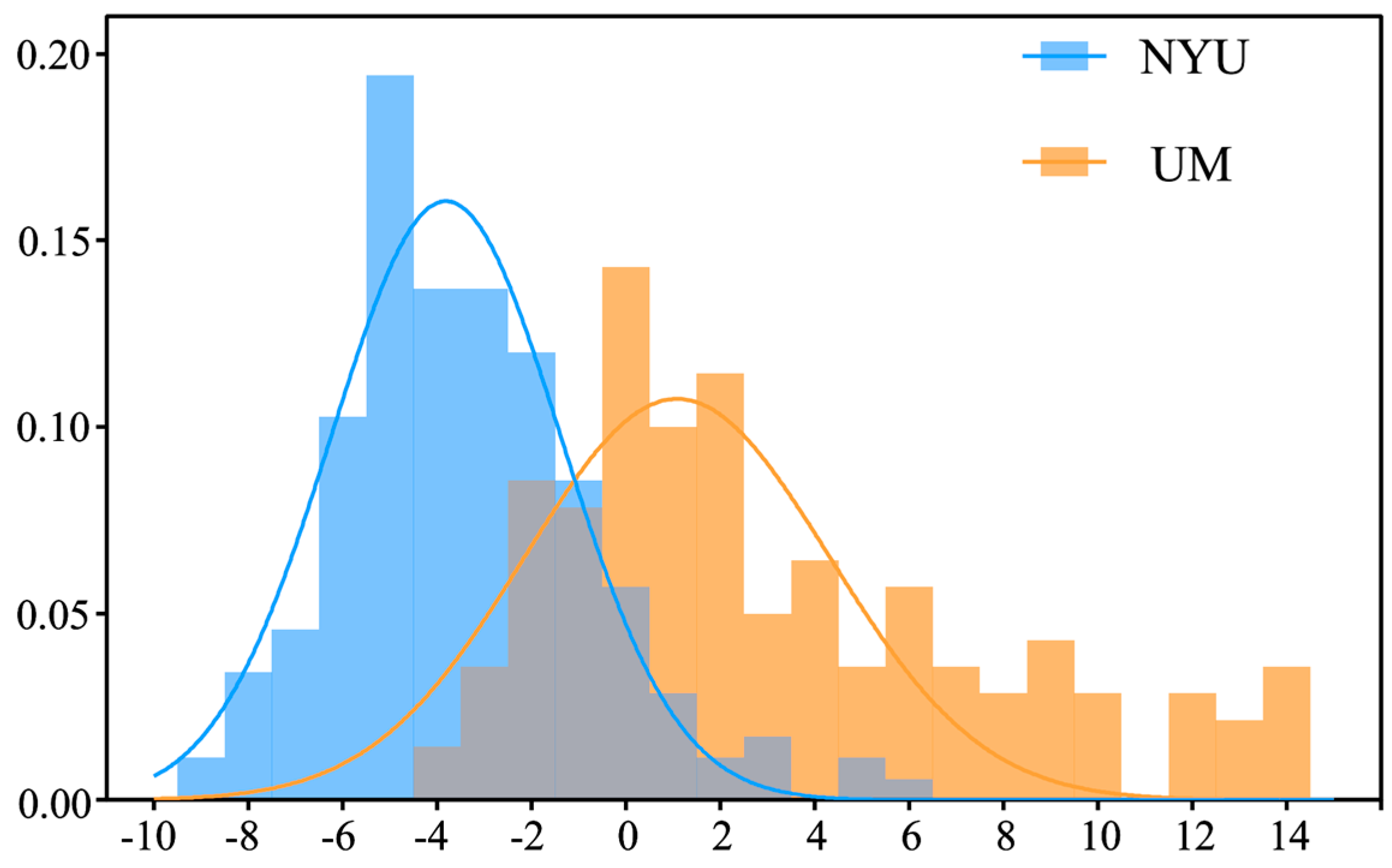
Figure 1 shows the data distribution of NYU Langone Medical Center (NYU) and University of Michigan (UM) sites in ABIDE dataset.
Table 1 shows the data distribution for the remaining 15 sites in the ABIDE dataset. Specifically, the first principal component of all subjects at two sites was obtained through PCA, and then the frequency distribution histogram of the first principal component of all subjects at each site was drawn. The PCA algorithm maps functional connections in a high-dimensional space to a low-dimensional space, where the first principal component is the direction of the maximum variance in the data and is the line that best illustrates the shape of the point group. Therefore, the first principal component can be used to reflect the distribution of functional connection data of different sites to the greatest extent. It can be seen that the data distribution of the different sites is heterogeneous.
2.2. rs-fMRI Data Preprocessing
The ABIDE dataset is derived from the abide dataset preprocessed by the preprocessed connectome project (PCP) [
21]. A configurable pipeline for analysis of connectomes (CPAC) was selected for the preprocessing pipeline. The steps include slice timing correction, head motion correction, intensity normalization, nuisance signal removals, band-pass filtered (0.01–0.1 Hz), standard spatial registration. A pre-processed fMRI scan data is a 4D time series, including three-dimensional space dimension and one-dimensional time dimension. The time series used the mean time series signal or BOLD signal of voxels within the region of interest (ROI) in the brain map. The brain mapping template we selected was Craddock 200 (CC200), with 200 ROIs defined. Pearson correlation coefficients were used to evaluate the functional connections between the mean time series of each ROI pair, resulting in a 200 × 200 functional connection for the CC200 brain map.
2.3. Multi-Site Anti-Interference Neural Network
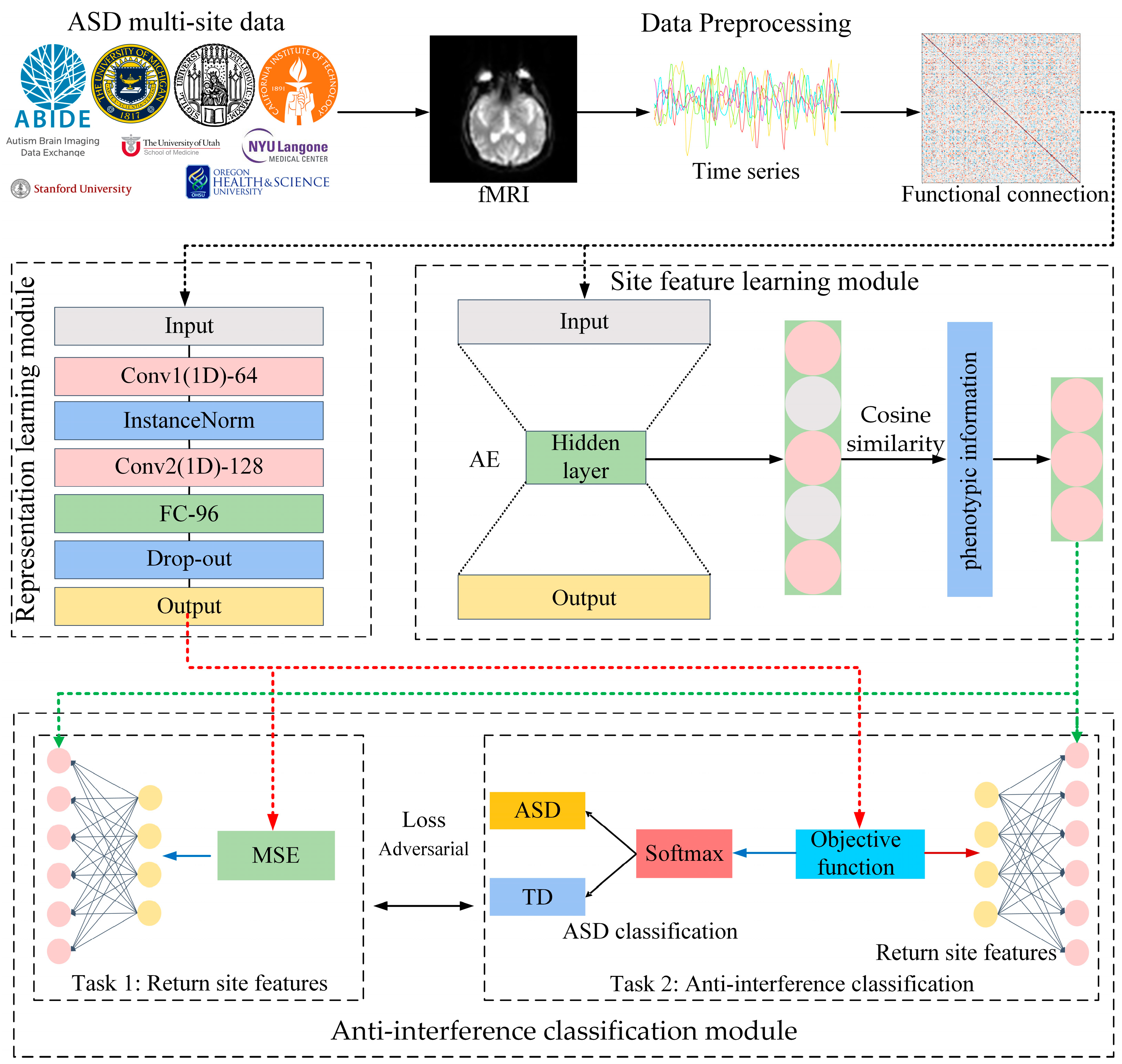
We propose a multi-site autism classification method with anti-interference neural networks (MS-AINN). MS-AINN is composed of representation learning module, site feature extraction module and anti-interference classification module, and adopts multi-task adversarial design. The overall architecture is shown in
Figure 2.
Firstly, multi-site fMRI images are extracted into functional connections after data preprocessing, and functional connections are used as input data for the model. Then, the site feature extraction module will extract site features from the functional connections of the subjects to quantify the heterogeneity between sites, and the site features will be used as labels in the multi-task. The specific process is to first extract low-dimensional subject level feature vectors through AE, then use site average pooling to calculate the mean vector of all subject level feature vectors in the site as site features, and finally select low-redundancy site features through phenotypic information correlation features.
After the above two parts of the process, we have the input data functional connection required for MS-AINN multitask design, as well as two kinds of labels, disease type labels and site characteristics labels that quantify site heterogeneity. MS-AINN can then be used for ASD classification training. Firstly, ASD classification features are extracted from functional connections through the representation learning module. Specifically, large-scale one-dimensional volume nuclei are used for feature extraction, because the weight of the convolutional nuclei corresponds to brain regions, and the importance of each brain region to ASD classification can be analyzed. The convolution result will be further classified through the Fully Connected Layer (FC) for further feature extraction. Then, the obtained classification features will perform two tasks of MS-AINN through the anti-interference classification module, which are site feature regression task and anti-interference classification task. The reason is that the objective function of the anti-interference classification task is composed of ASD classification loss and site feature regression loss. However, the direction of regression loss optimization in the anti-interference classification task is opposite to that in the site feature regression task, that is, the anti-interference classification task will increase the regression loss but the site feature regression task will reduce the regression loss. The anti-interference classification module performs two kinds of tasks with ASD classification features as input through the FC layer. When it comes to site feature regression, both tasks also use the same FC layer for regression.
MS-AINN adopts the training mode of alternating iteration of two tasks, and the updated parameters of each task are independent of each other and do not overlap each other. After the adversarial training of the two tasks, the model can effectively remove the influence of multi-site confounding effect (multi-site confounding effect refers to the confounding effect caused by the heterogeneity of multi-site data) on feature extraction of the representation learning module.
2.4. Site Feature Learning
We use autoencoder (AE) and site average pools to extract site image features from functional connections. The low-dimensional vectors reflecting the individual characteristics of the subject are obtained by using the autoencoder, and the average vectors of all individual feature vectors in the site are calculated by using the site average pool. From this, we can obtain low-dimensional feature vectors that can reflect site information. Autoencoder is a kind of feedforward neural network, which is composed of encoder and decoder, where the encoder encodes the input data
into a low-dimensional representation, as shown in Formula (1).
is the activation function,
and
are the weight and bias of the encoder, respectively. The decoder reconstructs the output of the encoder back to the original input data, as shown in Formula (2), where
and
are the weight and bias of the decoder, respectively.
The autoencoder completes the model training by minimizing the reconstruction Error. The loss function is the Mean Squared Error (MSE) between the input data and the reconstruction result . After the encoder completes the training, the output of the encoder can be regarded as a low-dimensional feature of the input data .
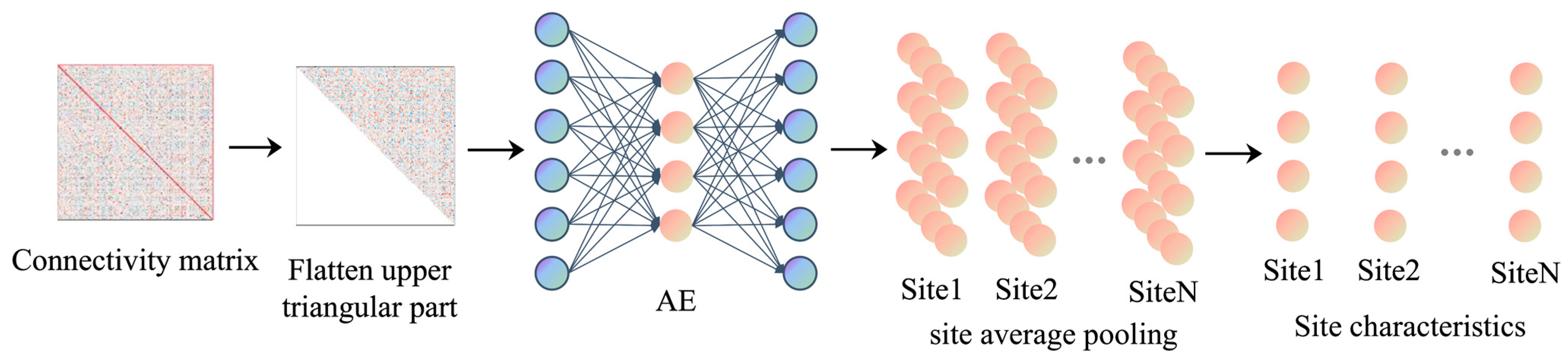
Using the characteristics of unsupervised training and nonlinear dimensionality reduction of the autoencoder, the low-dimensional individual feature vector of the subject is extracted first. Because the functional connection matrix is symmetric, the upper triangle part of the matrix is repeated with the lower triangle part. In order to reduce the parameter number of the autoencoder and speed up the training efficiency, the lower triangle part containing the main diagonal is deleted, and the upper triangle part is planar as a one-dimensional vector as the input of the autoencoder. The autoencoder adopts a single hidden-layer structure, and the encoder part and the decoder part are a single-layer fully connected layer. The autoencoder weights are 19,900 × N and N × 19,900, respectively, where N is the embedded dimension of the hidden layer, which is determined by hyperparameter optimization. The data of all site subjects are used as input to train the model, and the optimal model is saved in the position with the least loss value. Then, the output vector of the encoder is obtained by feeding the one-dimensional function connection vector into the autoencoder, which is a low-dimensional vector reflecting the individual characteristics of the subject. In order to further obtain the feature vector that can reflect the difference information of the sites, the mean vector of the individual feature vector of all subjects in each site is calculated by site average pooling. The reason is that we use the mean of individual characteristics of the subjects in the site to reflect the characteristics of a site as a whole. The process is shown in
Figure 3.
In addition to site heterogeneity in functional connections, site heterogeneity was also included in subjects’ phenotypic information. However, the amount of phenotypic information, such as age and gender, is much smaller than the number of site features extracted from functional connections. The dimension of the vector composed of phenotypic information may be single digits while the dimension of the feature vector extracted from functional connections is in the hundreds. Directly connecting the two vectors together may make it difficult to reflect the site heterogeneity contained in the phenotypic information. Therefore, we select features based on the cosine similarity between the site feature vector extracted from the functional connection and the phenotype information, so that the final site features contain the phenotype information indirectly. The site feature vector needs to calculate the cosine similarity with the phenotypic information of the site, so we use the mean and variance of the phenotypic information of all subjects in a site to represent the phenotypic information of the site. The way to calculate cosine similarity is to first arrange the mean and variance of phenotypic information of all sites into mean vector and variance vector, respectively, according to the order of sites, and then some dimensional features of all site feature vectors are formed into a vector according to the same site order. The form of the vector is the same as that of the mean vector and variance vector, and the cosine similarity can be calculated with the mean vector and variance vector, respectively. Finally, some dimensions with high cosine similarity are selected to form a new site feature vector.
The specific process Is to first calculate the mean and variance of the phenotypic information of each site, and then arrange the mean and variance of each site according to the sequence of a site, form the mean vector and variance vector, and standardize. The final vector form is N × 1, where N is the number of sites. The feature vectors of all image sites are arranged in the same order to form a site feature matrix of the form N × F, where N is the number of sites and F is the feature dimension. A one-dimensional vector (form N × 1) is selected along the dimensionality of the site in the site feature matrix, and the cosine similarity is calculated by means of the mean and variance vectors of the phenotypic information. The cosine similarity is calculated as shown in Equation (3), where
A and
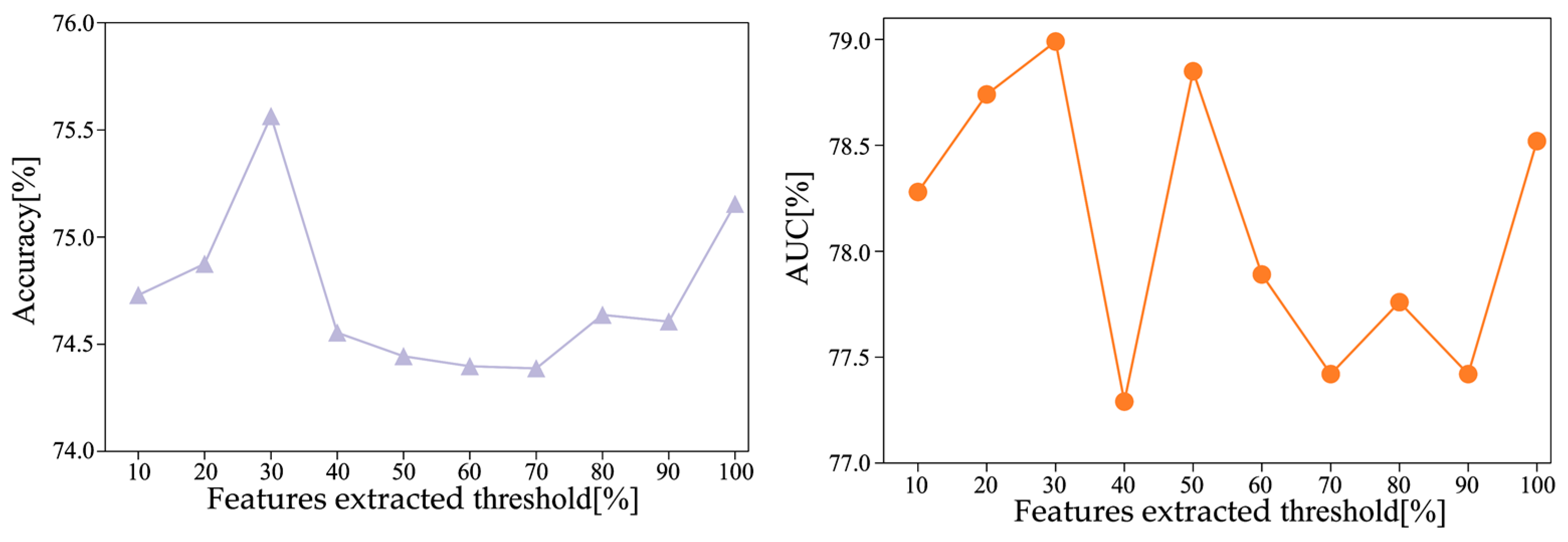
B represent two vectors. According to the cosine similarity, the similarity order of phenotypic information of each site can be obtained. In cases where the mean and variance vectors of multiple phenotypic information are ordered differently, we use a voting mechanism to determine the unique ordering. The higher the similarity ranking and the stronger the phenotypic information correlation, the more likely it is to reflect the site heterogeneity. Finally, the threshold is defined according to the top percentage of similarity ranking, and the features within the threshold range are selected to form a new site feature vector. Phenotypic information we selected included sex, age, full scale IQ, verbal IQ, and operational IQ. Through experiments, the features with the top 30% cosine similarity are selected as site features.
2.5. Representation Learning
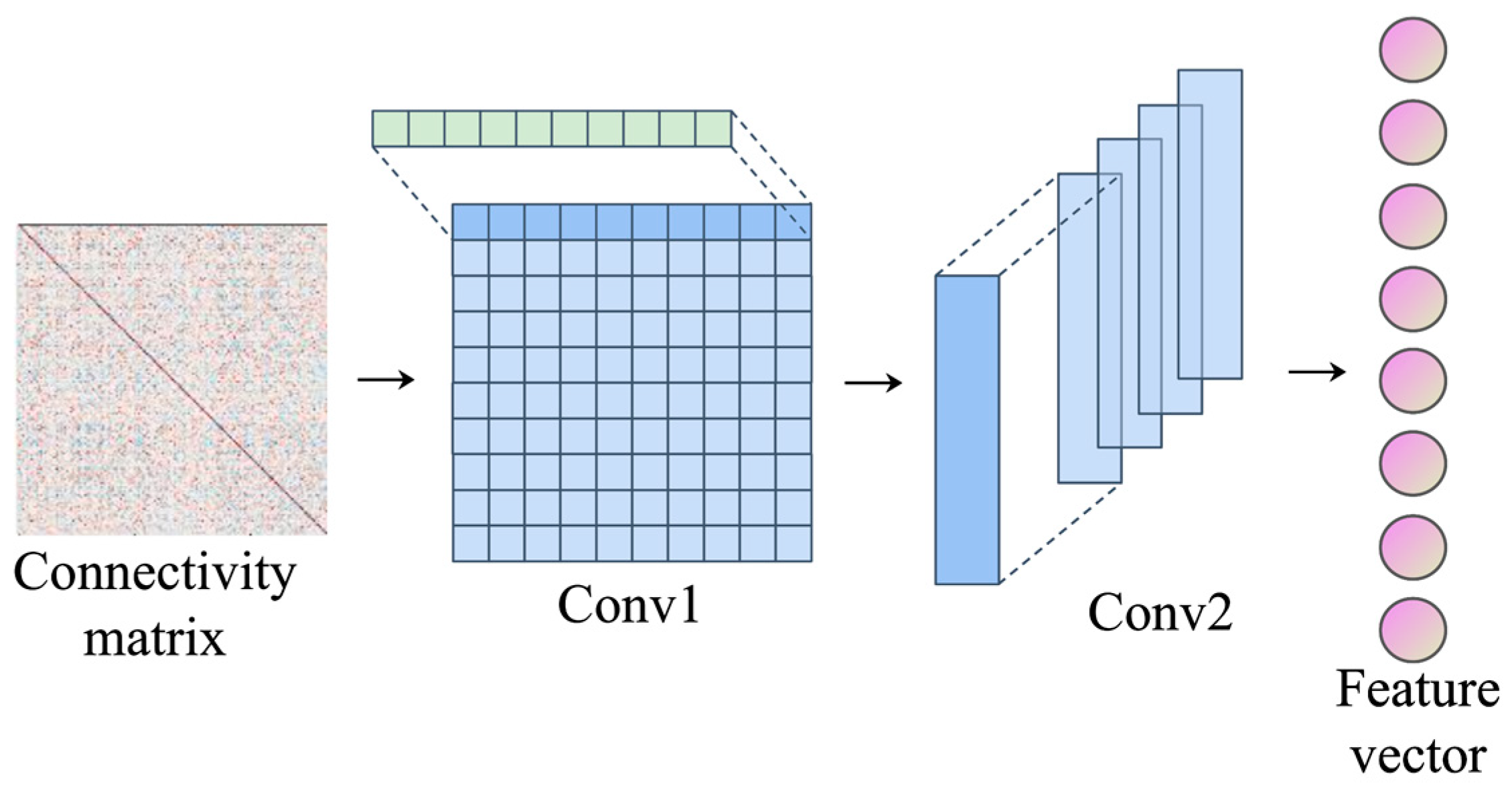
The input of the representation learning module is the functional connection matrix, and the physiological meaning is the brain functional network. There are obvious differences between the data structure and the picture, mainly reflected in the fact that the functional connection matrix is a non-Euclidean space and the picture is a Euclidean space. In the Euclidean space of the picture, the neighbors of a pixel are the surrounding pixels in space, so the convolution nuclear energy in the two-dimensional form gathers the information in the neighborhood domain. However, in the functional connection matrix, the neighbor nodes of the target node are not always adjacent in space, so the convolution kernel in two-dimensional form cannot guarantee that all the gathered information comes from the neighbor domain of the target node. This can lead to a mixture of features from different brain regions, which is not conducive to the analysis of important brain regions. The topology of the functional connection matrix is characterized by the fact that each row in the matrix represents the correlation between the brain region corresponding to that row and all the other brain regions. When the functional connection matrix is regarded as a brain functional network, a row in the matrix can also be used as the correlation between the target node and its neighbor node. Therefore, we designed the CNN (1D) representation learning module. The convolution kernel is one-dimensional and contains the same number of weights as the number of brain regions, so that the receptive field of the convolution kernel is exactly a row of the functional connection matrix, which can imitate the interaction between the target brain region and all other brain regions in the row. In this way, each convolution operation gathers the information of the neighbor domain of the target brain region, and the convolution results of each brain region are not mixed with each other, which is conducive to the final analysis of important brain regions. The CNN (1D) consists of two convolutional layers and one fully connected layer, as shown in
Figure 4.
The first layer uses the horizontal convolution kernel in the form of 64@1 × 200, where 1 × 200 represents the shape of the convolution kernel, 200 represents the number of brain regions, and 64 represents the number of channels. Since each row in the matrix represents the correlation between a certain brain region and all other brain regions, the convolution kernel in the form of 1 × 200 ensures that each operation is carried out between the target brain region and its adjacent brain regions, and the convolution result can be regarded as a feature of the target brain region. The feature form obtained after the first layer of convolution operation is 64 × 200 × 1, meaning 64 feature maps extracted from 200 brain regions. The second layer of convolution uses vertical convolution kernel to extract whole brain features from brain region features. The convolution kernel in the form of 128@200 × 1200 × 1 forms the feature convolution operation of 200 brain regions to form the feature of the whole brain, and the dimension is 128. In this process, the features of brain regions are mapped to the features of the whole brain, and the weight of convolutional nuclei corresponds to the weight of brain regions. Therefore, the absolute values can be used to represent the importance degrees of different brain regions, so as to analyze the interpretability of the model. Finally, the feature is further extracted through a full-connection layer to better complete the classification task. Pooling layer is not used in the model mainly because each convolution is independent of each other based on the unit of brain region, there is no overlap in the receptive field, and the redundancy of extracted features is small. On the contrary, some key features may be lost in the downsampling of the pooling layer. In addition, the purposes of sampling under the pooling layer are to reduce the amount of computation, to prevent overfitting, and to increase the receptive field of subsequent convolution CNN (1D). In order to ensure the corresponding relationship between convolutional kernel weights and brain regions, the range of receptive fields is always the same as the number of brain regions, and pooling of the previous layer is not required to increase receptive fields. At the same time, if the calculation amount is reduced by the pooling layer, the corresponding relationship between convolutional kernel weights and brain regions will be destroyed, resulting in the mixed features of different brain regions, and the importance of specific brain regions cannot be studied. Moreover, it has been proved that downsampling of the pooling layer does not necessarily improve the performance of the CNN network [
22]. The convolution operation is shown in Formula (4), where
is the output of the current layer,
is the output of the previous layer,
is the parameter of the current layer,
is the dot product operation of the corresponding receptive field, and
is the bias of the current layer.
Considering that the range of the functional connection matrix is −1 to 1, the representation learning module selects the activation function tanh with the same range. The classification layer uses Softmax function to calculate the probability of each category, as shown in Formula (5). The Dropout layer and L2 regularization are added to prevent overfitting of the model, while the InstanceNorm layer is used to normalize the features in each channel.
2.6. Objective Function and Model Training
In the existing methods, the model is trained in a zero-sum game way when adopting adversarial design, that is, the adversarial task that removes confounding effects is trained separately and its loss value is minimized [
19,
20]. This method is feasible when there is only a single task, such as the generation of adversarial network. However, when the target task and the adversarial task are inconsistent, the lowest loss value of the adversarial task may not make the target task achieve the optimal result, and may even have the opposite effect. Dinsdale et al. [
19] have found in the experiment that the adversarial task that removes scanner information can also cause adverse effects on the target task and reduce the final prediction performance. Therefore, MS-AINN does not train the adversarial task alone, but combines the adversarial task and the target task into an objective function, and completes the training of the two tasks simultaneously through the loss optimization of the objective function, so that the two can reach a balance in the training and ensure the performance improvement of the target task.
The objective function of anti-interference classification task is composed of loss functions of ASD classification and site feature regression. The purpose is to make the loss of ASD classification decrease while the loss of site feature regression increases, so as to complete the disease classification and site feature regression adversarials at the same time. Firstly, the symbols used in the function are introduced.
represents the functional connection of
N subjects.
represents the labels of
N subjects;
represents the site feature vector of
N subjects;
is the parameter representing the learning module;
is the classifier parameter;
is the regression component parameter. The loss function of site feature regression task is the mean square error, as shown in Formula (6). The classification task loss function is cross entropy loss, as shown in Formula (7).
The model adopts the training mode of alternating iteration. In each epoch, the regression task loss
is optimized first, and the regression component parameter
is trained. After optimization, the objective function loses
, and the representation learning module parameter
and classifier parameter
are trained. In order to realize the confrontation between two trainings, the objective function should minimize the classification loss
and also maximize the regression task loss
. Therefore, the regression task loss function is selected as the denominator of a fraction and the whole fraction is added to the classification task loss function. In this way, when the optimizer reduces the objective function
, the classification task loss
will also decrease and the regression task loss
will increase, as shown in Formula (8).
is a hyperparameter, which is used to balance the loss optimization of the two tasks, so as to prevent the excessive increase of
in the training of the objective function from resulting in too-strong restriction on the representation learning module and the degradation of the classification performance of ASD.
In the two trainings of the model, the first regression task trained a regression component to identify the site difference information contained in the features extracted by the representation learning module. The second anti-interference classification task training optimizes in the opposite direction through two kinds of losses, namely, classification and regression, so that the representation learning module can extract classification features while containing fewer features that can reflect the difference information of the sites. In this way, after two training and alternating iteration optimizations, the ability of the regression component to identify the site difference information is gradually enhanced, and the site difference information contained in the classification features extracted by the representation learning module is gradually reduced. In this way, the confounding effect brought by site heterogeneity will be weakened in ASD classification, and anti-interference classification will finally be realized.
4. Discussion
In this study, we propose an MS-AINN-CNN (1D) deep learning model, to classify ASD and TDS on large multi-site rs-fMRI data based on whole-brain functional connections. MS-AINN is composed of two key parts: (1) Site feature learning, which extracts site features from the functional connections of subjects by using AE, site average pooling and phenotypic information feature selection, so as to reflect the heterogeneity information among sites, and then uses it to build a mapping relationship with the representation learning features to provide necessary conditions for adversarial training against the impact of site confounding. (2) Anti-interference model training, using two tasks of site feature regression and anti-interference classification to reduce the site heterogeneity information contained in the representation learning features, so that the model classification is less affected by the multi-site confounding effect. The results show that when the representation learning module is CNN (1D), MS-AINN can reduce the accuracy of site classification of representation learning features, indicating that the impact of the representation learning module on the site confounders is weakened, which proves that MS-AINN can realize the representation learning to the site confounders. Moreover, all classification indexes of MS-AINN-CNN (1D) were improved, which proved that MS-AINN’s confounder remove representation learning successfully improved the model classification performance. In addition, the results of the representation learning module replacement experiment show that MS-AINN can also bring about the same disaggregation effect and obvious classification performance improvement when using MLP and CNN (2D) representation learning modules, indicating that anti-interference ideas play a key role in the entire, while the representation learning module provides a baseline performance for classification. Among them, MLP and CNN (2D) have lower classification effect than CNN (1D), which proves that large-scale convolutional kernel design considering physiological significance has superior performance in ASD classification research.
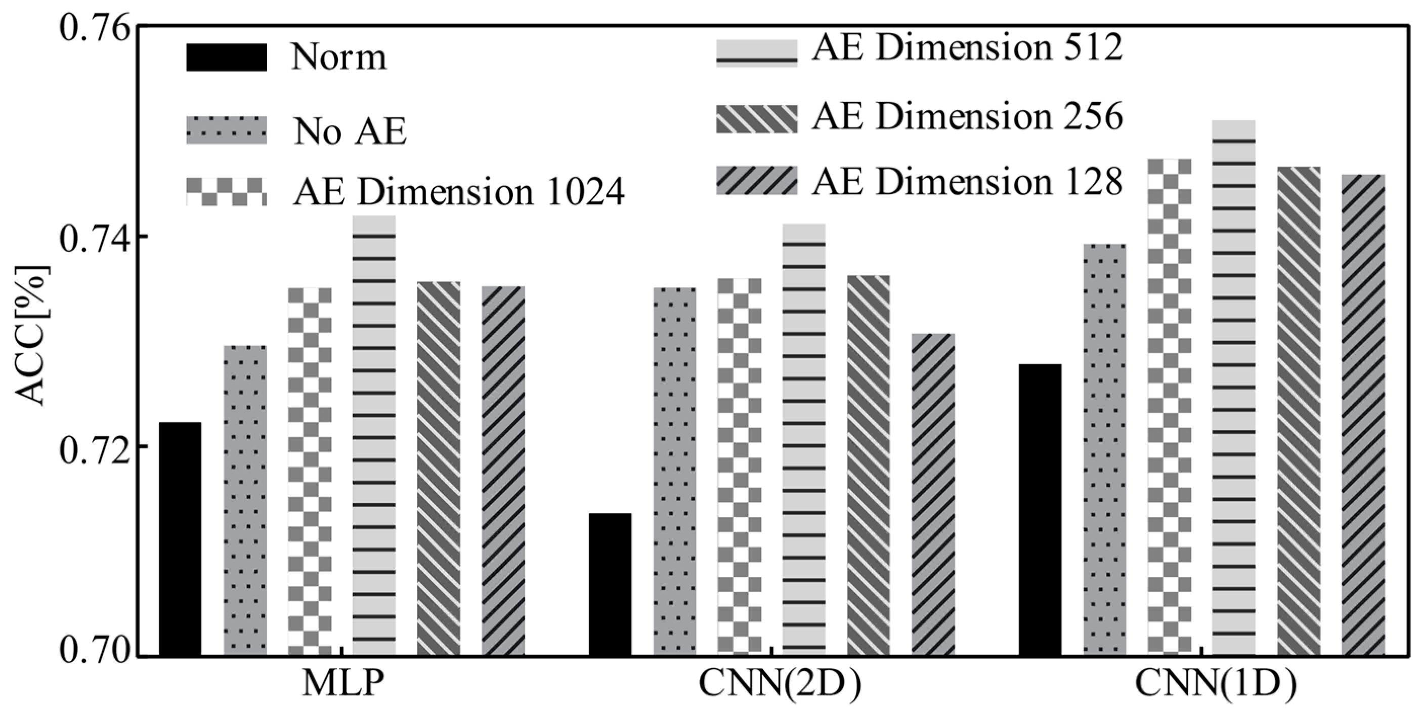
In the optimization results of AE hidden layer, the overall accuracy rate increases first and then decreases with the decrease in site feature dimension, because different parameters will obtain site features of different dimensions. When the dimension is large, there are more redundant features, and when the dimension is small, site differences cannot be fully expressed, and the optimal results cannot be achieved in both cases. In the site feature selection threshold experiment, the results show that with the change of feature selection threshold from low to high, the accuracy and auc increase first, then decrease and then increase, and the highest accuracy is 75.56%, auc is 78.99% when the threshold is 0.3. The reason is that when the threshold is low, the features selected are high-scale related features, which are composed of site image features and potentially contain phenotypic information, and have a strong ability to reflect the difference between sites. Therefore, the increase in such features can enable MS-AINN to more accurately realize the impact of site confounding, and the classification accuracy will therefore increase. The threshold value of 0.3 to 0.7 is the decline range of accuracy. At this time, there are fewer features related to the high scale in the site features. With the increase in the threshold value, the redundant features begin to increase, and the effect of the confounding remove begins to decline, and the accuracy also declines. The threshold value of 0.7 to 1.0 is the interval where the accuracy rate rises again. The reason is that among the site image features extracted from AE and site average pooling, there are still features that can highly reflect the difference between sites except the features with high phenotypic information correlation. The distribution of these features has nothing to do with phenotypic information correlation, but only increases with the increase of the total number of features. When a certain threshold is exceeded, the number of features in this part is enough to enhance the ability of site features to reflect site differences again, and ultimately improve the accuracy.
The experimental results of hyperparameter optimization show that different parameters will affect the classification accuracy, and there is an optimal parameter to make the accuracy highest. However, it can be seen from the experimental results that the accuracy difference between different parameters is small, and the accuracy difference between whether MS-AINN is used or not is large. Even when AE reduction and feature selection are not used, MS-AINN still has performance improvement. Therefore, it can be concluded that the reason for the effectiveness of the proposed method lies in the use of MS-AINN, and the purpose of the method is not to find the optimal parameter set, but to achieve anti-interference classification by means of the method of multi-site confounding removal.
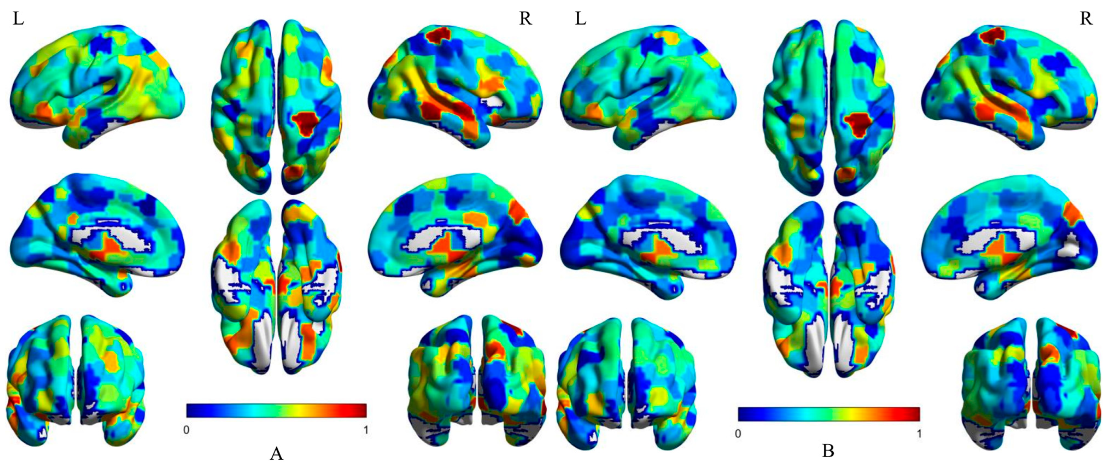
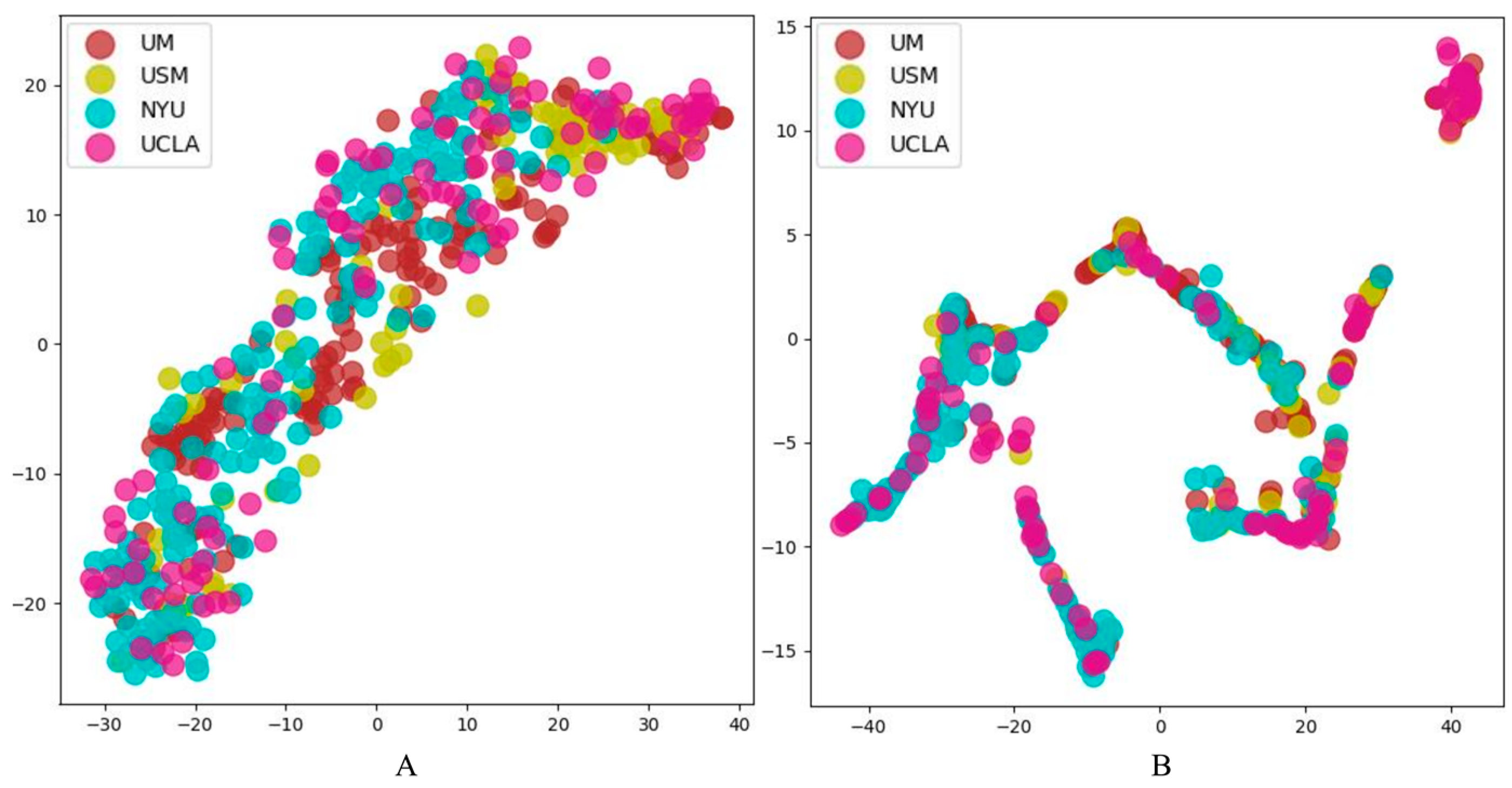
In the interpretability analysis of the model visualization, the results of the visualization of important brain regions show that the representation learning module can actively identify the brain regions that have changes due to disease, and extract the difference features for classification. Moreover, the high-contribution brain areas after using MS-AINN were the same as before, indicating that although MS-AINN limited the feature extraction of the representation learning module to remove site confusions, it did not affect the model’s recognition of important brain areas. At the same time, parts of the brain that were bluer became bluer and less important. MS-AINN also makes the representational learning module focus more on important brain regions that may have physiological differences, while ignoring non-important brain regions. After reducing the weight value of non-critical brain regions, the features extracted contain the difference information of normal patients in important brain regions, and reduce the interference of confounding factors in non-important brain regions, and finally improve the classification performance. The T-SNE visualization of the representation learning features shows that MS-AINN can make the features separated from each other gather together. The reason for the change in spatial distribution is the heterogeneity of the data of multiple sites. The feature extraction directly through the representation learning module will be affected by this, resulting in the separation of the feature vector domain between sites. In order to extract the feature vectors of the mixed influence of the sites, MS-AINN limited the feature extraction process of the representation learning module by means of adversarial training, so that the solution space of the model was concentrated in the region that did not reflect the differences of the sites, and finally obtained the feature vectors of the inter-site domain aggregation.
5. Conclusions
We proposed a multi-site anti-interference neural network ASD classification method that aims to make the representation learning results reflect the disease differences while being less affected by site confounding factors, and finally realize anti-interference classification. The experimental results show that the MS-AINN achieves the purpose of confounding the site. At the same time, the improvement of various classification indexes shows that reducing the impact of site confounders on representation learning can effectively improve the classification performance of models. Moreover, the MS-AINN can still improve the classification performance after replacing the representation learning module, which proves the universality of the architecture. Therefore, the MS-AINN that takes site confounders into account is of great significance for the design and research of deep learning ASD classification model under multi-site datasets.
The purpose of our method is to remove the multi-site confounding effect on ASD classification, which is realized by alternating iterative training of site feature regression task and anti-interference classification task under MS-AINN. This training method can limit the feature extraction of the representation learning module, so that the extracted features are less confounded by the site. However, it is found in the experiment that the restriction representation learning module will not only weaken the confounding effect of the sites, but also affect the classification. Neither too large nor too small restriction can achieve the optimal performance. Therefore, hyperparameters are required in the objective function to balance the losses of the two tasks, which also increases the difficulty of parameter adjustment. In addition, we only test classification tasks on ASD datasets, and the next step will be to test other tasks on different multi-site datasets.


