Article

Real-Time Interval Type-2 Fuzzy Control of an Unmanned Aerial Vehicle with Flexible Cable-Connected Payload

1
Department of Automatic Control and Systems Engineering, University of Sheffield, Sheffield S1 3JD, UK
2
Control and Automation Department, Istanbul Technical University, 34467 Istanbul, Turkey
*
Authors to whom correspondence should be addressed.
Algorithms 2023, 16(6), 273; https://doi.org/10.3390/a16060273
Submission received: 30 April 2023 / Revised: 20 May 2023 / Accepted: 24 May 2023 / Published: 29 May 2023
(This article belongs to the Special Issue Algorithms for PID Controller 2023)

Abstract

:
This study presents the design and real-time applications of an Interval Type-2 Fuzzy PID (IT2-FPID) control system on an unmanned aerial vehicle (UAV) with a flexible cable-connected payload in comparison to the PID and Type-1 Fuzzy PID (T1-FPID) counterparts. The IT2-FPID control has significant stability, disturbance rejection, and response time advantages. To prove and show these advantages, the DJI Tello, a commercial UAV, is used with a flexible cable-connected payload to test the robustness of PID, T1-FPID, and IT2-FPID controllers. First, the optimal coefficients of the compared controllers are found using the Big Bang–Big Crunch algorithm via the nonlinear UAV model without the payload. Second, once optimised, the controllers are tested using several scenarios, including disturbing the payload and the coverage path planning area to examine their robustness. Third, the controller performance results are evaluated according to reference achievement and point-based tracking under disturbances. Finally, the superiority of the IT2-FPID controller is shown via simulations and real-time experiments with a better overshoot, a faster settling time, and good properties of disturbance rejection compared with the PID and the T1-FPID controllers.

1. Introduction

Significant and rapid advances in unmanned aerial vehicle (UAV) technology have made them economically viable and easily maintainable. They have been used in research and in civil, military, and commercial applications, such as military UAVs, search and rescue, and agriculture [1,2,3,4,5]. Even though they can complete tasks, they still face many challenging problems because of the sensor accuracy and the coupled highly nonlinear system dynamics. Considering the controller of the UAV, which is one of the challenging problems, encouraged many researchers to take on such challenges and propose several control designs, such as proportional–integral–derivative (PID) [6,7], fuzzy PID control (FPID or T1-FPID) [8,9,10], linear quadratic regulator (LQR) [11,12], linear quadratic Gaussian and loop transfer recovery (LQG/LTR) [13], model predictive control (MPC) [12,14,15] and H∞ [16,17] control algorithms.
The controller algorithms and the calculation of their parameters are directly related to the physical dynamics of the system. However, the physical dynamics of the UAV represent a challenge for many of the control algorithms implemented on these UAVs, mainly when the control parameters are determined by using limited known dynamic model parameters. Moreover, knowing all parameters of the physical dynamics is almost impossible due to uncertainties or inaccessible parameters. Therefore, the stable controller parameter might cross to the unstable region in the presence of uncertainty or inaccessible parameters. To explain and illustrate the problem, it is scaled and tested using a mini UAV. For indoor experimental research, nano or mini UAVs have proven their efficiency concerning easy access, small sizes and weights [18]. As a result, researchers have used several commercial UAVs, such as Bitcraze Crazyflie 2.0 [8,19,20,21,22], Parrot Mambo Minidrone [9,10,12] and DJI Tello [23,24,25].
In many studies, the connection with the payload represents a further research challenge [23,26,27,28]; the control problem under uncertain payloads is solved using reinforcement learning. The UAV has a flexible cable, payloads, and magnets. When using the magnets, the payloads can connect to UAV. Hence, the weights cannot be known, adding additional uncertain parameters. Thanks to model-based meta-reinforcement learning, the system’s inputs and outputs are trained and created model-based data using a human-based remote controller. After designing a model-based meta-reinforcement learning dynamic model, a model predictive control algorithm is implemented to cope with such effects [23].
UAVs face other challenges not only due to the payload but also due to wind disturbances. In [27], a path following a control algorithm for a UAV with cable-connected payload is designed under wind disturbances. In addition, near hovering and cruising states are included in the control, as well as an employed position-based tracking control algorithm for the outer structure. A whole system model is developed with payload and disturbance effects, meaning that they are not unknown parameters in [27]. Considering unknown parameters, such as the payload mass, an excellent example of associated research work can be attributed to [26] on adaptive UAV control for a cable-suspended unknown payload. The system is tested with a nonlinear and adaptive PD controller. The coefficients/parameters of the UAV controllers are tuned via many different optimisation methods [29], and each of them has its advantages and disadvantages. In [30], a comparative study of different controllers for UAVs is investigated in terms of limitations and strength parts. In this study, we focus on fuzzy-based PID controllers since they have better accuracy than PID controllers and are computationally efficient, which makes them applicable to UAVs in real time [7].

Contributions

This study shows the successful implementation of the Interval Type-2 Fuzzy PID (IT2-FPID) controller under a nonlinear dynamic model and unknown/uncertain parameters of the UAV with a payload in simulation and real-time systems. The implementation comes from model-based tuned parameters to overcome an unknown weighted flexible cable-connected payload. It is aimed to eliminate the oscillating payload effect on DJI Tello UAV and to follow the given references by using these controllers. PID, T1-FPID, and IT2-FPID are tuned using the Big Bang–Big Crunch (BB-BC) optimisation method [31] on the dynamical model of the UAV without a payload. Due to the unmodelled dynamics, such as inaccessible parameters or uncertainties, the controller coefficients are fine-tuned on a real-time UAV without the payload before being tested with the flexible cable-connected payload. After that, it is expected that the UAV will be able to eliminate disturbing payload effects and demonstrate efficient tracking of the designed trajectory. Moreover, the performance of the IT2-FPID is compared with T1-FPID and PID under the same scenarios. The presented results of the study clearly show that the designed IT2-FPID control system is superior in comparison to its T1 and conventional counterparts. The video file provided in the Supplementary Material shows the real-time control performance of the deployed IT2-FPID.
The rest of the study is organised as follows: Section 2 provides the UAV model, including the DJI Tello model and the problem statement and challenges. Section 3 presents implemented controller methods, which are PID, T1-FPID and IT2-FPID, and the simulation results. Then, Section 4 shows the indoor testing area and the designed offline path. Moreover, the process of position localisation of the UAV is explained in this section. The real-time results of the PID, T1-FPID and IT2-FPID controllers are given in Section 5. Finally; Section 6 presents the conclusions and a perspective on future work.

2. UAV Model and the Problem Definition

This section presents the mathematical model for the dynamics of DJI Tello UAV, and the problem statement and challenges. The first part of this section describes the dynamic model of the UAV. This dynamic model is shown without any payload. After that, the problem of the UAV with a flexible connected payload is explained.

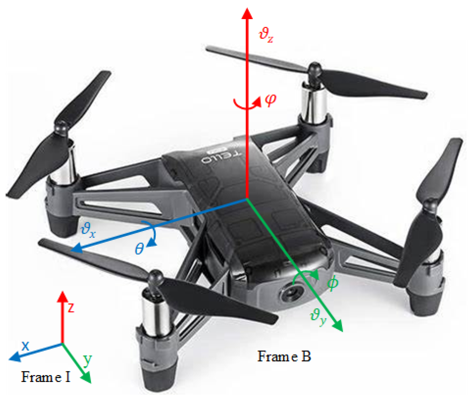
2.1. Model Dynamics of DJI Tello UAV

Before outlining the UAV model, we show the main coordinate frames used in this study: ( . ) I represents the global Earth-fixed Earth-centred inertial frame, and ( . ) B is the body-fixed frame, fixed at the UAV centre of mass (CoM) as given on Figure 1. There are two types of configurations for the UAV, which are × and + configurations [8,20,32]. In this study, the ×-type UAV is modelled and used.
The position ( p I ) and attitude ( η I ) of the UAV with respect to the frame I are defined as follows:
p I = x y z T , η I = ϕ θ ψ T , υ I = p ˙ I = R υ B , ω I = η ˙ I = T ω B ,
where the vector p I contains the x, y, and z Cartesian position coordinates of the UAV inertial frame, and υ I and ω I are the derivative of position and attitude values, respectively. The superscripts ( . ) I and ( . ) B denote, respectively, the inertial and body frames. The η I vector contains the angles of roll ϕ , pitch θ , yaw ψ of the UAV body frame, R is a rotational matrix, and T is a translation matrix used in frame conversions. These rotation and transformation matrices are used to calculate the transformation of the inertial frame to the body frame or vice versa. The rotation and transformation matrices are written in Equation (A1) of Appendix A.
The υ variable is used to represent the linear velocity, and ω is used to represent the angular velocity. In this study, the heading angle of the UAV, yaw reference ( ψ r ) is equal to ψ r = 0 in order to overlap the inertial and the body coordinate frames of the DJI Tello.
After the defining position and orientation, a nonlinear dynamic equation for the DJI Tello UAV can be written with the Newton–Euler formulation as given below [8,20]:
m uav υ ˙ I = F I = F g r a v i t y I + F t h r u s t I , I B w ˙ B = w B × I B w B + τ r o t o r B .
In Equation (2), m uav is the mass of the UAV to the CoM of the UAV, F g r a v i t y I is the gravity force, F t h r u s t I is the total thrust force which comes from the propellers, I B is a moment of inertia, and I B is referred to as the inertia matrix. The cross product at the right-hand side of the angular velocity dynamics equation comes from the Coriolis force effect. Considering the DJI Tello UAV, this effect can be ignored because of the size of the UAV. Ref. [8] tested a fixed heading angle and ignored the Coriolis effect on the DJI Tello UAV, which has an almost similar size to the DJI Tello UAV. Therefore, the formula can be written as I B w ˙ B = τ r o t o r B , and the UAV torques ( τ r o t o r B ) are expressed by τ ϕ , τ θ , and τ ψ , respectively:
F g r a v i t y I = 0 0 m uav g T , F t h r u s t I = R F t h r u s t B .
To overcome the gravity effect, the force is applied to the CoM of the UAV as F g r a v i t y I . The acceleration due to Earth’s gravity is denoted as g. The F t h r u s t I forces are generated by propellers, and the formula is written as Equation (4). The angular velocity of each rotor’s propeller is denoted as Ω i , and the thrust coefficient is referred to as b
F t h r u s t B = 0 0 b i = 1 4 Ω i 2 T ,
υ ˙ I = x ¨ y ¨ z ¨ = b m uav i = 1 4 Ω i 2 = s ( ϕ ) s ( ψ ) + c ( ϕ ) s ( θ ) c ( ψ ) s ( ϕ ) c ( θ ) + c ( ϕ ) s ( θ ) s ( ψ ) c ( ϕ ) c ( θ ) 0 0 g .
In Equation (5), s ( . ) and c ( . ) denote the sine and cosine, respectively. In the equations above, the nonlinear dynamical model for the translational motion of the UAV is represented, and a detailed linear dynamical model of the UAV is written in Equations (A5)–(A7) of Appendix A. The angular velocity dynamics of the UAV also can be found in Equations (A3) and (A4). As aforementioned about the mass of UAV ( m uav ), it only gives the UAV weight.
In the above equations, mass equals m uav = 0.08 kg, and the length between the CoM and propeller is 0.6 m. The detailed parameters of the DJI Tello UAV are explained in Refs. [24,34].

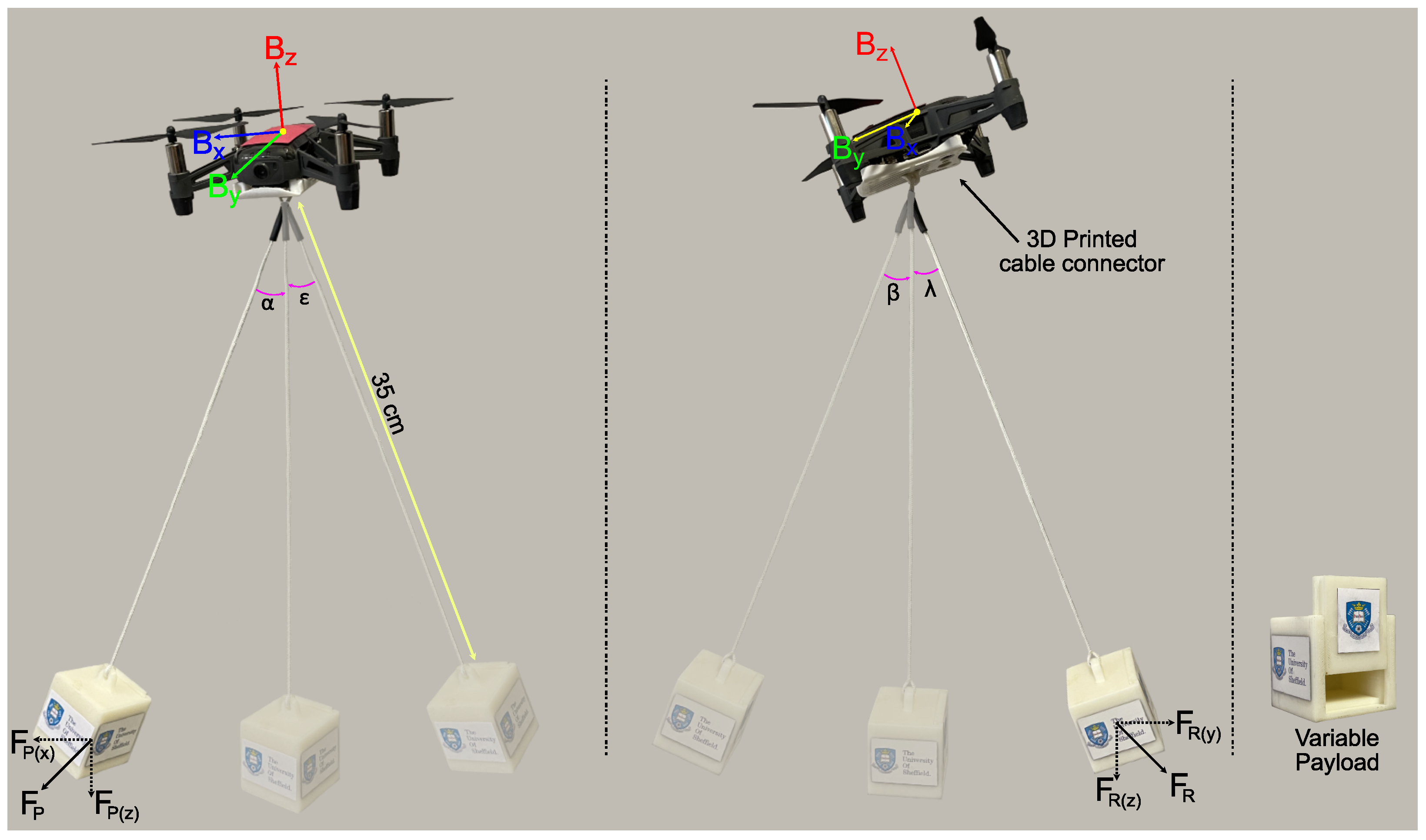
2.2. Problem Statement and Challenges

In Figure 2, the UAV with the flexible cable-connected payload and its pendulum effects are shown. The figure shows the different perspectives of the UAV with cable-connected payload and the variable payload in detail. A 3D-printed part is created and mounted to provide a UAV connection with a payload cable. The cable length is 35 cm and is chosen as flexible. Taking into account the pendulum effects, forces F P , F R and the angles α , ε , β , and λ vary with the acceleration of the UAV due to Newton’s second law. The maximum carrying payload is measured with empirical methods, and its maximum value is determined as 75 g for the experiments. This weight ( m p ) is a significant value when considering the mini UAVs. Then, it is able to rewrite the equations as m total = m uav + m p . Instead of rewriting the dynamical equations and calculating the controller parameters using swinging m total , we propose that the compared controllers can eliminate the unknown payload effects and the variable CoM problems without redesigning or the calculation.
Understandably, unknown payloads and disturbances directly relate to the system dynamics. Therefore, the main objective of this work is to overcome these adverse effects. At this point, instead of re-writing the equations of the UAV dynamics and redesigning the controllers by considering the whole mathematical model with the additional dynamics of the swinging payload, the controllers are designed by considering the known dynamics of the UAV itself without taking the payload and disturbance effects into account so that the robustness of the three controllers is compared with each other, then the IT2-FPID controller gives the results in terms of system stability and robustness.
The most important question is as follows: why do we focus on uncertain parameters, such as unknown payload and flexible cable effects? This system is a simulation of a commercial agricultural UAV problem. Commercial agricultural UAVs may contain liquid or other payloads. However, the problem is that these payloads, such as seeds or pesticides, are unknown loads because of their variable weights and variable centre of masses during the flight.

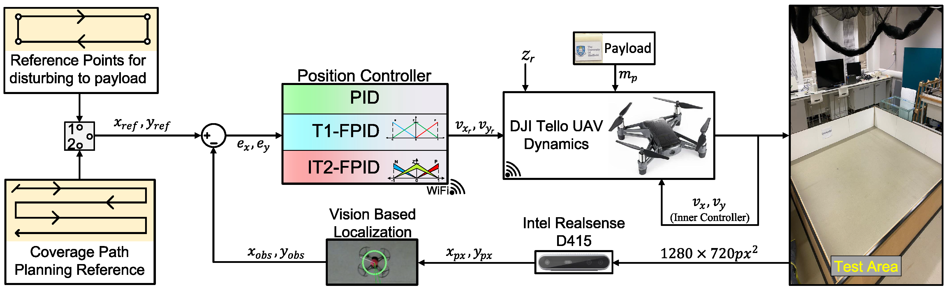
3. Implemented Controllers

In this study, we design and deploy PID, T1-FPID and IT2-FPID controllers as x-y position controllers that generate the x-y velocity reference signals υ x , υ y (m/s) to be tracked by the on-board velocity controller by DJI Tello UAV. In this context, let us first define the position errors to be minimised by the controllers on the x and y axes e x , e y as follows:
e x = x r e f x o b s e y = y r e f y o b s
where ( x r e f , y r e f ) and ( x o b s , y o b s ) are the references and the feedbacks (actual position of the UAV), respectively. In this study, the reference and feedback units are in meters (m) in the position-based controller. To minimise e x , e y , we designed two controllers that generate the velocity signals u x = υ x , u y = υ y . Within the scope of this study, we do not handle the altitude z and yaw ψ control problems of the UAV and use the onboard controller directly. Throughout the study, we set altitude reference z r e f = 90 cm and heading angle reference of the UAV ψ r e f = 0 .
In this section, as the x-y position controllers have the same structure, the subscripts ( x , y ) in e x , e y , u x , u y are dropped in the rest of the section for a better understanding.

3.1. PID Controller

The PID control law for the UAV is represented as follows:
u = K c e + 1 T i e d t + T d d e d t ,
where u is a reference signal for the inner controller, e is represented as the error, and T i , T d , and K c are the integrator, derivative, and proportional gain, respectively.

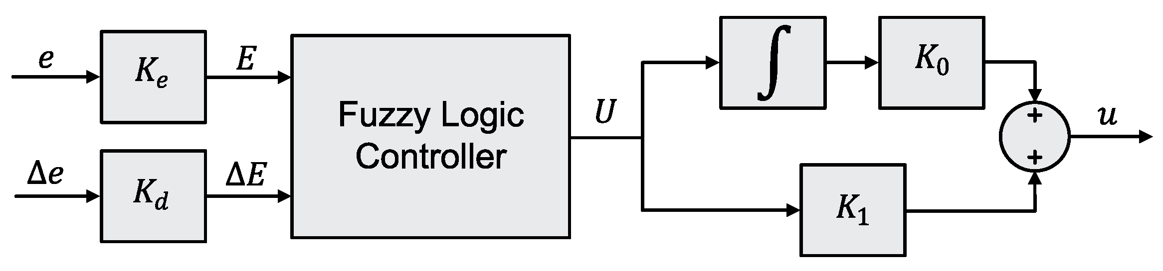
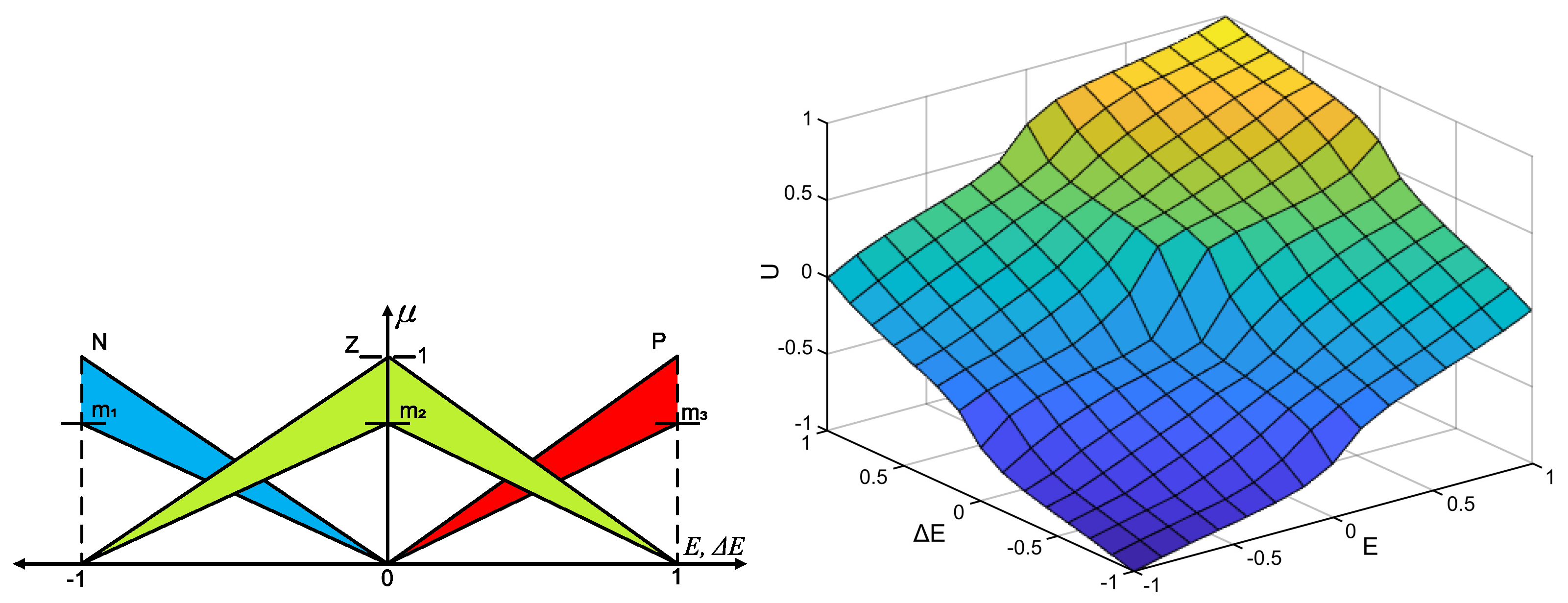
3.2. Type-1 Fuzzy PID Controller

In this section, the general structure of the T1-FPID is presented. Before starting T1-FPID, the fuzzy PID control block for T1 and IT2 is shown in Figure 3 [35]. The position error (e), and its rate of change ( Δ e ) are shown as controller inputs [8,9].
As shown in Figure 3, the input scaling factors (SFs) are denoted as K e and K d , while the output scaling factors (SFs) are denoted as K 0 and K 1 . The equation is in the form
E = K e e , Δ E = K d Δ e ,
where E and Δ E denote the FLC inputs. The output of the FLC (U) is transformed to the actual control signal of the T1 or IT2 fuzzy PID controllers (u) as follows:
u = K 1 U + K 0 U d t .
The employed fuzzy logic controller (FLC) is designed with 3 × 3 rules as given in Table 1. The consequent part of the rules is described with crisp singletons. Moreover, they are represented with five linguistic fuzzy terms, which are defined as follows: PB—positive big; PM—positive medium; Z—zero; NM—negative medium; and NB—negative big.
In Figure 4, the membership functions (MFs) of the T1-FPID are presented for the UAV [8,9]. There are three MFs in T1-FPID, N, Z and P abbreviated from “negative”, “zero”, and “positive”, which are the linguistic fuzzy variables. The antecedents are defined with uniformly distributed symmetrical triangular MFs. In this study, triangular MFs are selected instead of Gaussian or other types of MFs. Triangular MFs provide a fast computational time and real-time implementation [7]. Moreover, the MFs values are determined based on empirical evaluations. The resulting control surface is shown in Figure 4. The implemented FLC uses the product implication and operates the centre of sets defuzzification method [36,37,38]. In this study, the fuzzy weighted average defuzzification method is used, and the equation is written as Equation (10):
U = i = 1 M y i f i i = 1 M f i
where U is the final output of the Takagi–Sugeno–Kang fuzzy inference system [39], f is the firing function of T1-FPID, y is denoted as consequent MFs, and M is the total number of rules. Table 1 is used for T1-FPID.

3.3. Interval Type-2 Fuzzy PID Controller

Just like the T1-FPID controller, the IT2-FPID controller is composed of choosing E and Δ E as inputs and the control action of the IT2-FLC U as output as displayed in Figure 3. The IT2-FLC has the same N = 9 rules and is presented in Table 1. The MFs of IT2-FPID are characterised by triangular MFs, and the control surface of the IT2-FPID is given in Figure 5. The linguistic fuzzy variables are N, Z, and P, respectively. Here, m n is the only parameter that creates the footprint of the uncertainty of the IT2-FPID [40]. We employ the following parameters: m 2 = α and m 1 = m 3 = 1 α as suggested in [36,40,41,42]. Therefore, the selection of the parameter ( α ) is vital because it directly affects U.
Several methods have been used for the calculation of the controller output (U) [40,43]. In this study, the Biglarbegian–Melek–Mendel method is used [40]. The equation relating to this method is given as follows:
y ¯ = i = 1 M f h i y i i = 1 M f h i y ̲ = i = 1 M f l i y i i = 1 M f l i U = ζ y ̲ + ( 1 ζ ) y ¯ .
where y i shows consequent MFs, M is the total number of rules (Table 1 is used for IT2), ζ is a weighting parameter for the type reduced set ( [ y ̲ , y ¯ ] ), and U is the output of FLC. Lastly, f l and f h are defined as the lower and upper firing functions of IT2-FPID, respectively. In Figure 5, the control surface, which selected ζ = 0.25 and α = 0.25 for IT2-FPID, is illustrated.
Parameters of T1-FPID and IT2-FPID are selected aggressively by using rule-based FLCs and MFs. The ζ and α parameters are selected by trial and error so that an aggressive control surface is created for IT2-FPID, then it is defined as ζ = 0.5 and α = 0.25 in the study. After that, a comparison of the control surfaces ( Δ U ) of the T1-FPID ( U T 1 ) and IT2-FPID ( U I T 2 ) is presented in Figure 6, taking into account their aggressiveness and smoothness. The differences between them are formulated as Δ U = U T 1 U I T 2 . An aggressive control action is characterised by a relatively higher control action output compared to the others. Specifically, if a line lies above another line in the positive region where E , Δ E 0 (or below in the negative region where E , Δ E < 0 ), the resulting control action is deemed aggressive. Conversely, if this condition is not met, it is deemed a smooth control action.

3.4. Optimisation Results and Simulation

All implemented controllers are optimised via the BB-BC algorithm, described in Appendix B. The cost function of BB-BC is defined as
ISE = ( e x 2 + e y 2 ) d t .
In the equation above, errors are defined for two axes as e x , e y of the UAV. The error values are explained in Equation (6), and integral square error (ISE) is selected for the performance criteria of the optimisation algorithm. In the BB-BC algorithm, the population size is chosen as 50, and the maximum iteration number is selected as 200 for the optimisation process of each controller. The BB-BC optimisation algorithm is used to tune K c , T i , and T d for the PID controller, and the K e , K d , K 0 , and K 1 parameters for fuzzy-based controllers are tuned using BB-BC, separately. It is noticed that α and ζ are defined empirically. The BB-BC approach evaluation over simulated data is performed within the Matlab environment [44]. The computation times for the controllers are measured between 1 and 4 ms; these values are negligible considering the sampling time in real-time and simulation experiments. The selected controllers and their parameters are in the Python environment [45]. Control signals υ x and υ y are constrained between 12 m/s and 12 m/s during the BB-BC search.
In Table 2, parameters of the controllers and the best performance criteria (ISE) obtained by BB-BC are listed. For tuning to the parameters of each controller, the position reference points are x r e f = 1.1 m and y r e f = 0.52 m for BB-BC optimisation.
The optimised controllers are tested on the simulation model, and the results can be seen in Figure 7. In the simulation, the reference signals are defined as 1.1 m for the x-axis and 0.52 m for the y-axis. They are the same as the references given in the controller parameter optimisation process using BB-BC.
These simulation results show that the IT2-FPID controller leads to the best results, with no overshoot, the slightest steady-state error, and the rise time. In addition, T1-FPID gives a smoother response than the PID controller. Considering the compared controllers, they do not have the same system responses in both axes due to the fact that the feedbacks of the UAV in both axes have different levels of noise. The aim of choosing different levels of noise is that the payload is not connected to the CoM of the UAV, and it will have a directly different effect on the axes. Oscillation and steady-state errors seen in Figure 7 are caused by the Gaussian disturbances added to the simulation model in the testing stage to show the robustness of the compared controllers against external disturbances. Gaussian distribution parameters for the x and y axis are defined as N ( 0 , 5 ) and N ( 0 , 15 ) , respectively. After testing the controllers in the simulation, the controllers are implemented in the UAV.

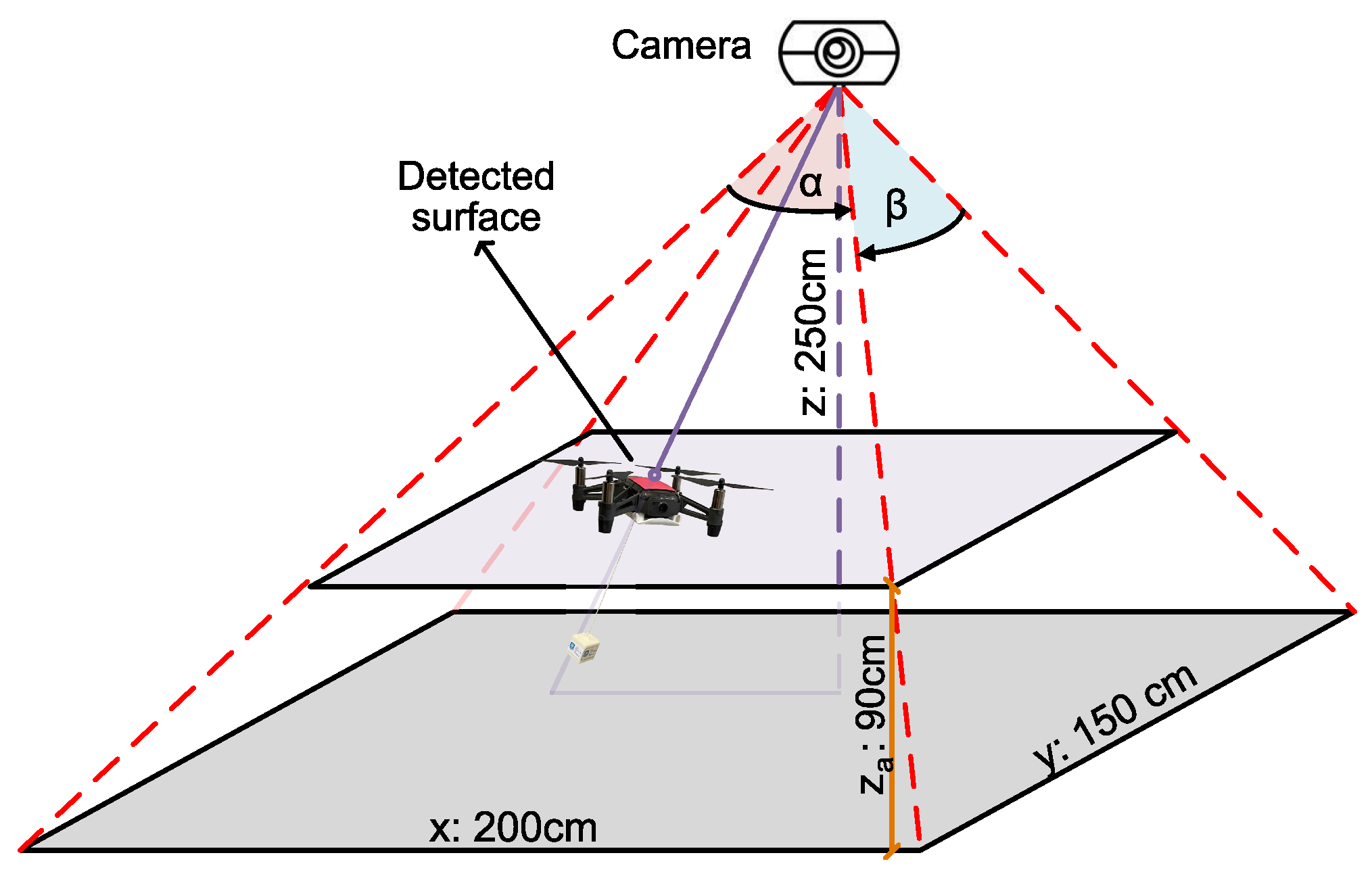
4. Indoor Testing Area

In Figure 8, an overview of the system, including the proposed IT2-FPID-based position controller, is shown. Figure 8 presents the overall structure of the system, including the proposed IT2-FPID-based position controller. Reference signals and controls and position estimates are calculated on the computer controlling the UAV remotely. The computer used in the real-time experiments has Intel i7 CPU, 32 GB RAM and NVidia GTX 1650Ti GPU. The generated outputs of the computer are the reference signals of the UAV. Moreover, the Python 3.10 environment is used in the system [45]. The computer and the UAV communicate via a Wi-Fi communication protocol. The design process of the main system starts with the generation of the reference signals for the desired UAV trajectory. Considering the main system, the process starts with the reference path generation. There are two different reference points in the proposed approach. The first one is about disturbing the payload. It means that when the UAV tracks the reference points using a stick, it is disturbed, and the flex cable-connected payload is a disturbance. Then, the second test is initiated as coverage path planning (CPP). Next, the offline CPP is explained, and the resulting reference points are given [46,47,48]. The last part is about how to detect the UAV position with a camera and vision-based localisation algorithm. In the following two sections, these are explained intensively.

4.1. Intel RealSense Depth Camera and Vision-Based Localisation Method

In this study, an Intel RealSense depth camera is used for the experiments [49], as it is a low-cost localisation system [8,50]. There are several advantages to using this particular depth camera in terms of its size, camera specifications and 3D Cartesian coordinate detection. Moreover, it has a 69 × 42 ( α × β ) field of view (FoV) for the RGB sensor, 1280 × 720 px 2 resolution, and a 30 fps RGB frame rate.
To find the localisation of the UAV, RGB colour detection is used to track it. A red-coloured circle piece is put on the region of interest of the area, and the colour parameters are measured as shown in Table 3. These colour parameters are in the hue, saturation, and value colour space (HSV). Moreover, the HSV values have maximum and minimum limits, which are shown in Table 3.
After detecting the HSV parameters, some trigonometric formulas are used to find the transformed centre points of the UAV. Figure 9 shows the three-axis sizes of the testing area ( x , y , z : 200 , 150 , 250 , respectively), camera position, UAV altitude level ( z a : 90  cm), and detected surface on the UAV.
In Equation (13), the raw centre points of the UAV ( x ^ p x and y ^ p x ) are defined, which are converged to the transformed centre points. In the matrix, s x , s y , s h x , s h y and t x , t y stand for scale factors, shear factors, and translation factors, respectively. Moreover, these parameters are determined by using “Computer Vision Toolbox for Matlab” [44] and using the following model:
x ^ p x y ^ p x 1 = s x s h y 0 s h x s y 0 t x t y 1 x p x y p x 1 .
Normally, this calculation is set for the two axes because the z-axis is fixed. For the calculation for the three axes, the trigonometric formula is used via Equation (14). In this equation, M x and M y show the total number of pixels for the x-y axes, and also σ x and σ y are defined as the relative mounting angles of FoV. Lastly, h (or z-axis) is used for the distance between the camera and the ground or floor. In Figure 9, the x-y-z-axes dimensions are given as 200 cm, 150 cm, and 250 cm, respectively, and by accounting for the following relations:
x o b s = z tan σ x + β y ^ p x / M x 1 , y o b s = z tan σ y + α x ^ p x / M y 1 .

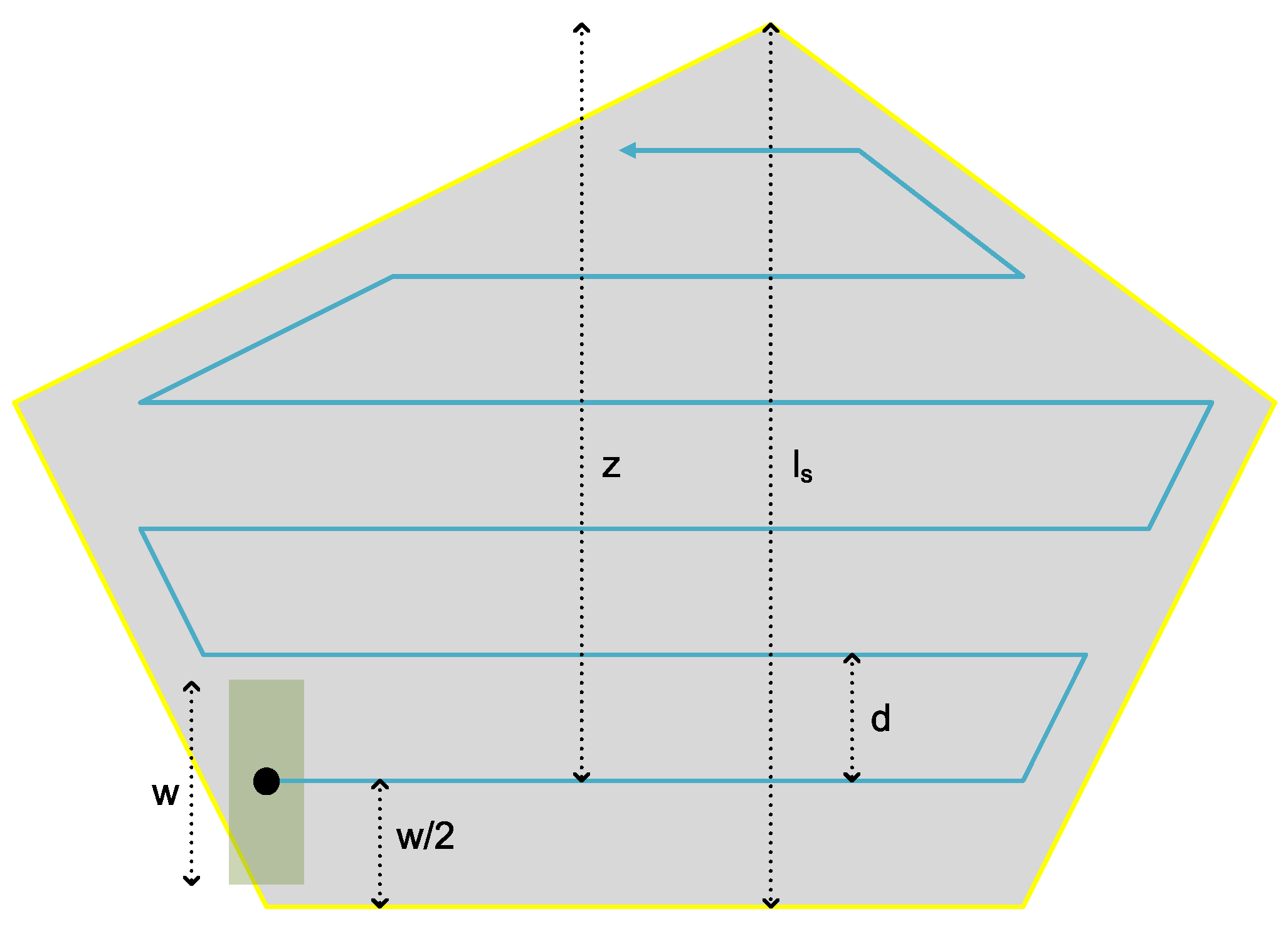
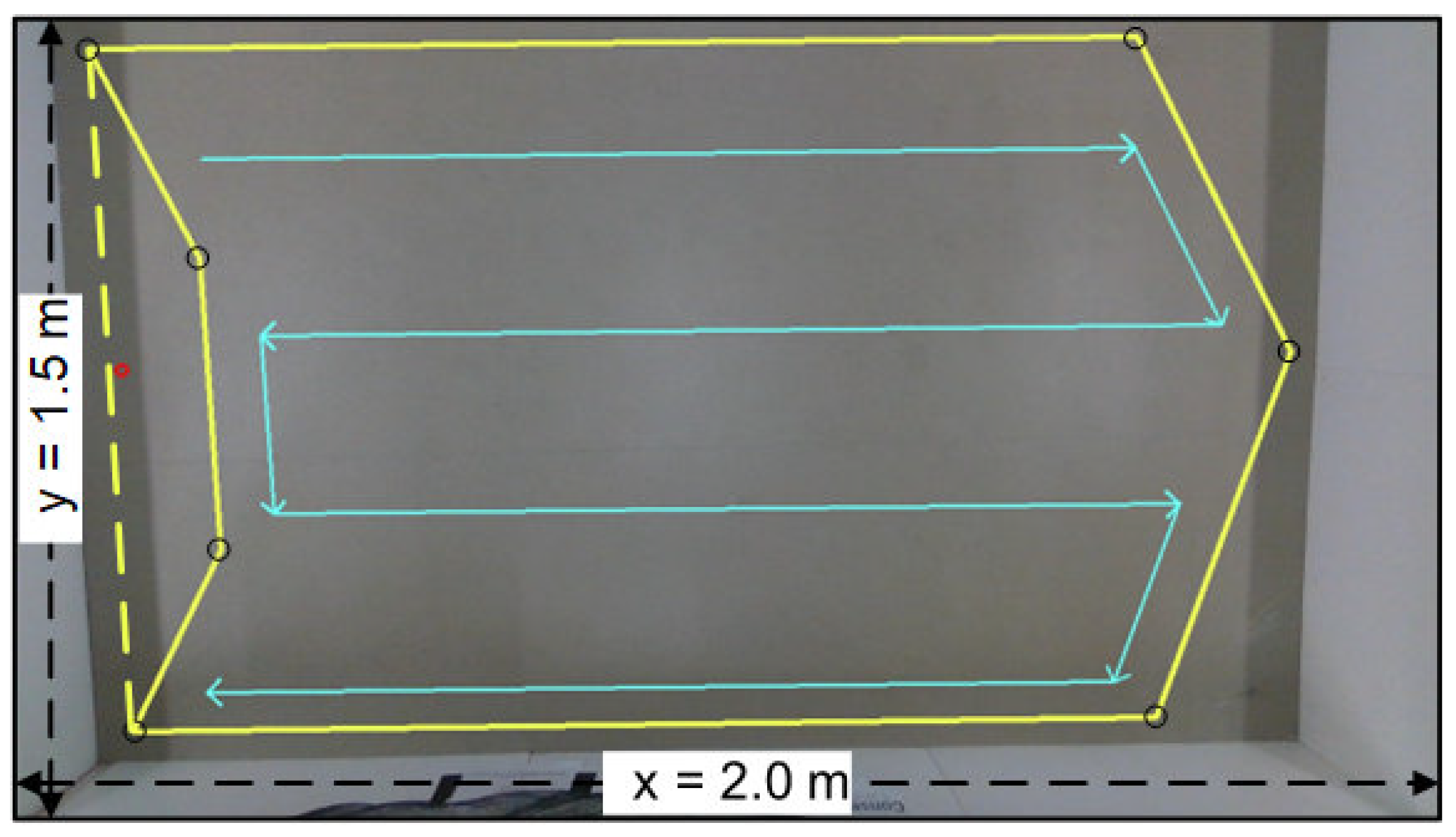
4.2. Coverage Path Planning

This section presents the implemented CPP algorithm. CPP is another challenging problem for UAVs  [46,47,48]. The UAV aims to track the specific points defined by using the CPP method.
In Figure 10, the boundaries, starting point, and the specific reference of the CPP lines are shown and coloured yellow, black, and turquoise, respectively. This is because the UAV has a task: reaching the specific points, which are the endpoints of the path segments. The following relation is used:
d = w . ( 1 υ ) .
The shape, length, and direction of the path constructed by the CPP algorithm depend on d, w, and l s values, and these correspond to the distance among rows, the half of the camera footprint, and the width of the original polygon, which is swept, respectively, and the percentage of vertical overlap between the width of the camera footprints on consecutive rows are denoted by υ and with a total number n of turns equal to
n = 2 . z / d if ( z mod d ) w / 2 , 2 . ( z / d + 1 ) if ( z mod d ) > w / 2 .
The total number of turns n resulting from the CPP algorithm is given in Equation (16), and this algorithm aims to minimise n to some degree, as it can be seen that this number depends on the z value, which is a function of the polygon width that is z = l s w / 2 . Therefore, the direction in which the polygon width is defined determines the value of n.
If the gap between the last row of the created path and the vertex or the edge of the original polygon is greater than half of the camera footprint w, then an extra row is added to the end of the path to reduce the gap as mentioned earlier; therefore, the distance between the last row and the original polygon might be less than w / 2 . In Figure 11, the difference between the distances from the border of the polygon to the initial row and the last row of the CPP path is an example of this case. The optimal line sweep direction and the path are determined by the following algorithm given in Algorithm 1 [46,47].
Algorithm 1 Basic CPP algorithm.
Step 1: (Farthest vertex v from the edge e)
For each edge, find the farthest vertex with respect to Euclidean distance and keep this (e, v) pair and the calculated distance value.
Step 2: (Minimum distance pair (e,v))
Compare the distance values and find the (e, v) pair which gives the minimum distance value.
Step 3: (Orthogonal direction vector)
The optimal line-swept direction is the vector that is orthogonal to the edge from the (e, v) pair found in Step 2, and the rows constructed by the CPP algorithm will be parallel to this edge e.
Step 4: (Path construction)
The path is defined by the way points that are connected by line segments. These way points are placed in such a way that the line segments connecting them are parallel to the edge on which the polygon width is defined and the distance between a way point and the border of the polygon satisfies the camera footprint requirements.
The CPP algorithm is employed in the testing area offline as shown in Figure 11. After reference-point generation by the CPP algorithm, all the controllers implemented in this study are tested over the area.
In the following section, the training and the testing results of the compared controllers are given, and it is shown that the best performance results are obtained by the IT2-FPID controller.

5. Real-Time Experimental Results

In this section, the performance of the IT2-FPID controller is compared with the PID and the T1-FPID controllers by the data gathered from real-time experiments. All experiments are in two parts: without/with disturbance and payload on the set-point tracking. The tuned parameters without payload using the BB-BC algorithm are employed in the UAV. After that, the set-point tracking shows all the results of the compared controllers under the flexible cable-connected payload and disturbance effects. Comparison results for these controllers are shown as root mean square error (RMSE) values. The sampling time ( T s ) is chosen as 055 ms. The selected optimal value of T s and the UAV IP address are communicated via Wi-Fi from the computer to the UAV. The latencies are taken into consideration, and these have a minimal impact on the real-time algorithm performance. The performance of the proposed approach can be observed via the video file provided as Supplementary Material.
The implemented controllers are tested for three cases. First, the UAV tracks the set point without any disturbance and the payload. Secondly, the controllers try to stabilise the system under disturbance and the payload. Additionally, the square reference points are given to the UAV. The last case is giving the reference path for the UAV by the CPP algorithm. In the CPP scenario, any external disturbance is not applied because when UAV follows the reference trajectory, the flexible cable-connected payload may generate disturbances on both axes due to the fact that the payload is not connected to the CoM of the UAV.
Disturbing the payload aims to investigate the controller responses under disturbance. In the last test, CPP aims to compare the controller performances for minimum time and maximum accuracy. Disturbing the payload and the CPP results show the robustness of the controller in real-time.

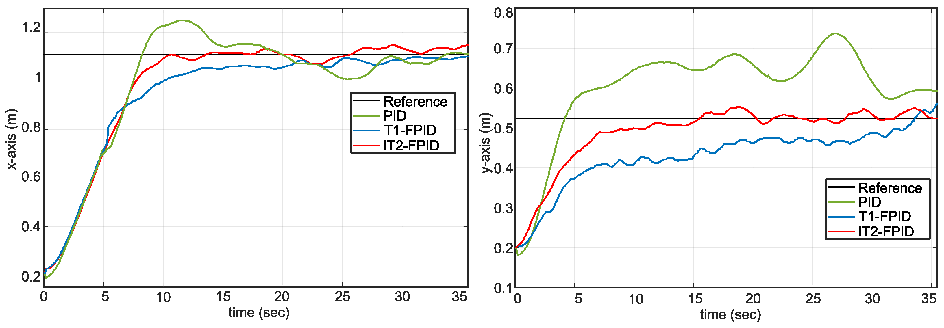
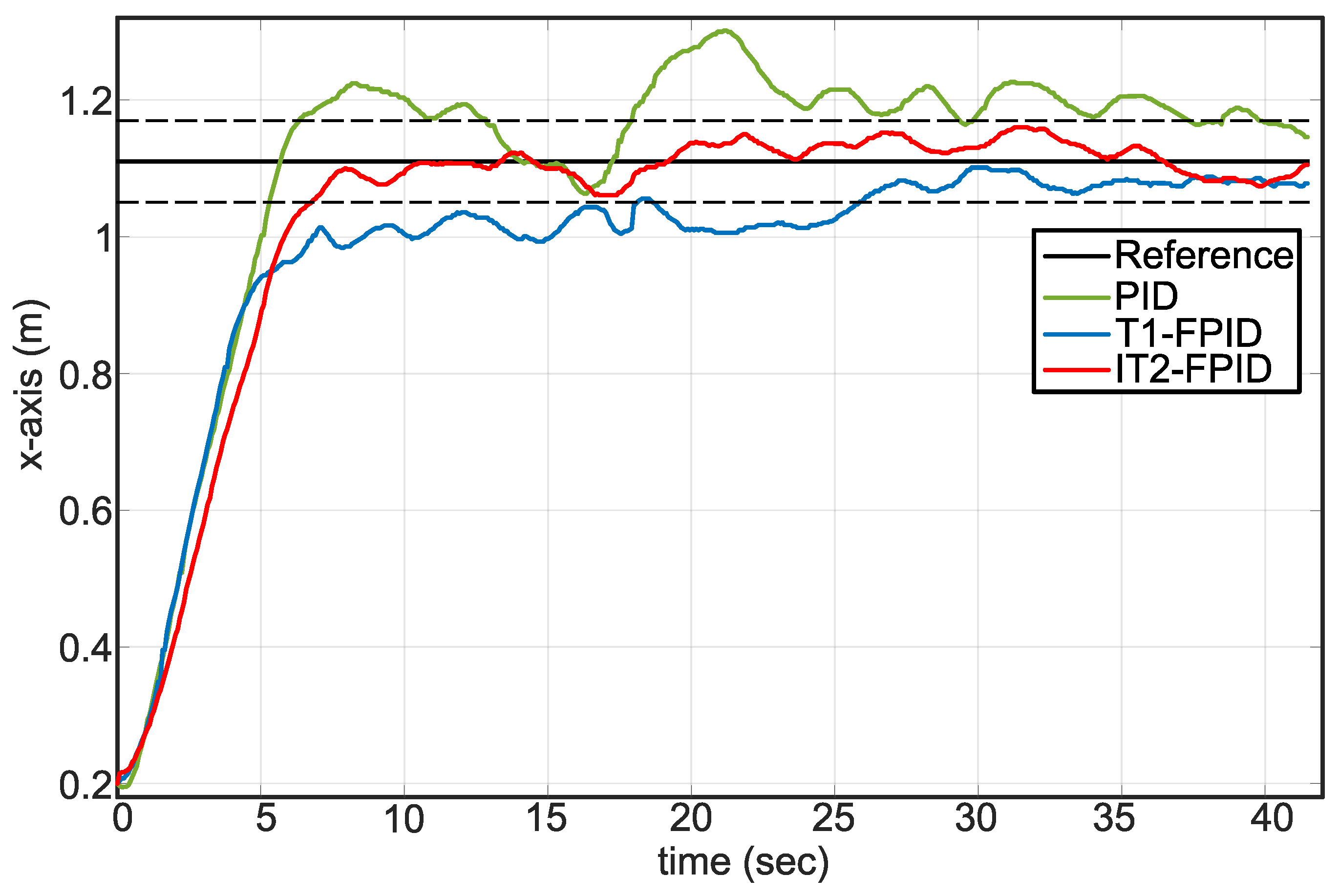
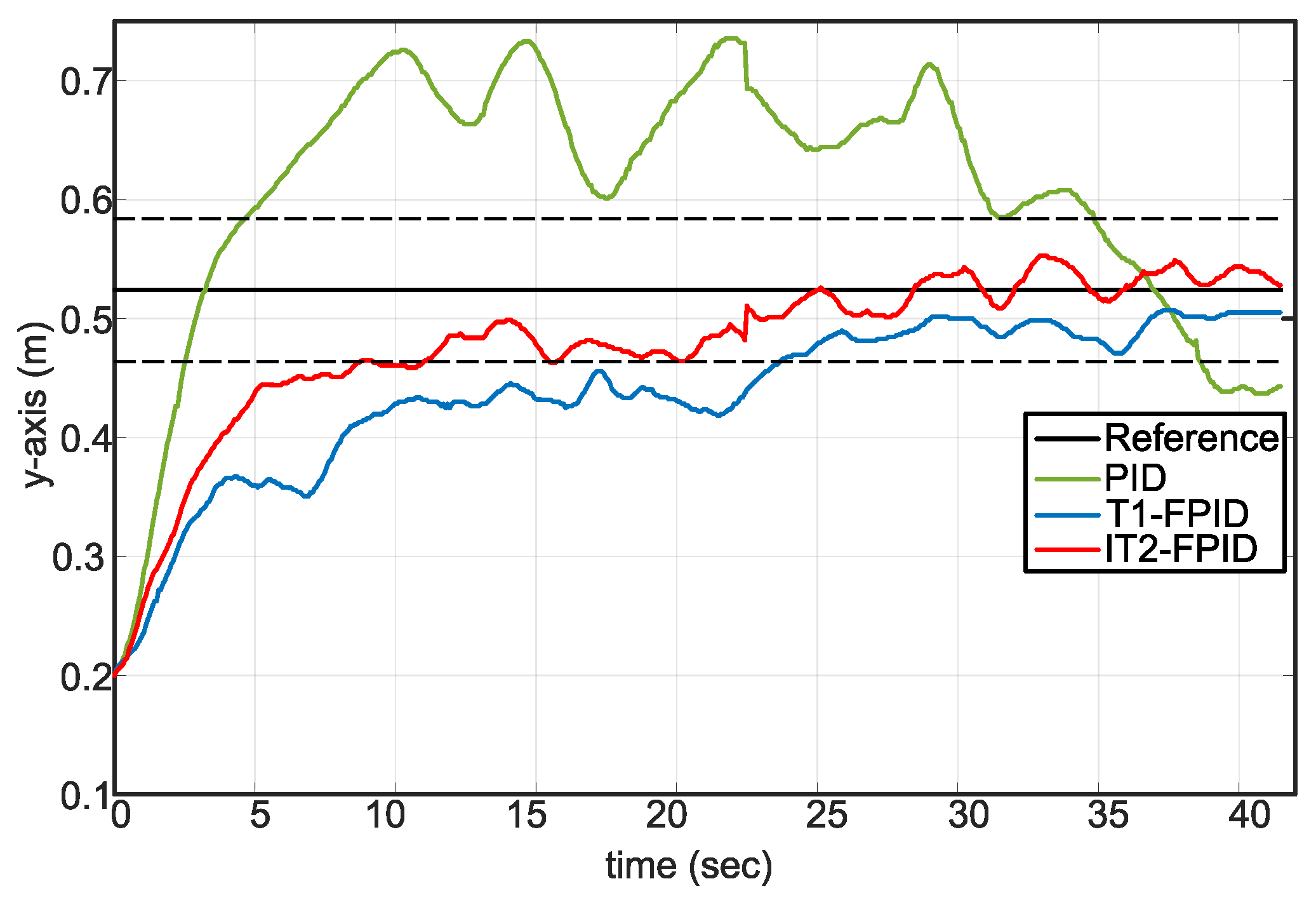
5.1. Set-Point Tracking without Disturbance and the Payload

Before testing with the unknown payload, all control methods and their control parameters are tested without a connected payload. The reason for this is that the defined controller parameters may need further fine-tuning.
In Figure 12 and Figure 13, the PID, T1-FPID and IT2-FPID position results can be seen. The reference, PID, T1-FPID, and IT2-FPID are coloured black, green, blue, and red, respectively. The starting point of the UAV is selected as x 0 = 0.2 m , y 0 = 0.2 m, and the reference points are chosen as x r e f = 1.1 m , y r e f = 0.52 m.
In Figure 12, the IT2-FPID results show the best performance compared to other controllers regarding settling time, oscillation, steady-state error, and overshoot. PID gives more overshoot and then arrives at coverage of the reference area after 31 s. T1-FPID has a slower response compared with IT2-FPID, but it also reaches the reference faster than PID.
In Figure 13, unlike the results on the x-axis, all the controllers do not achieve good results on the y-axis. Significantly, the PID controller has an overshoot problem and does not reach the reference or converge to the circle. Moreover, IT2-FPID looks faster than T1-FPID, and the system response is the best.

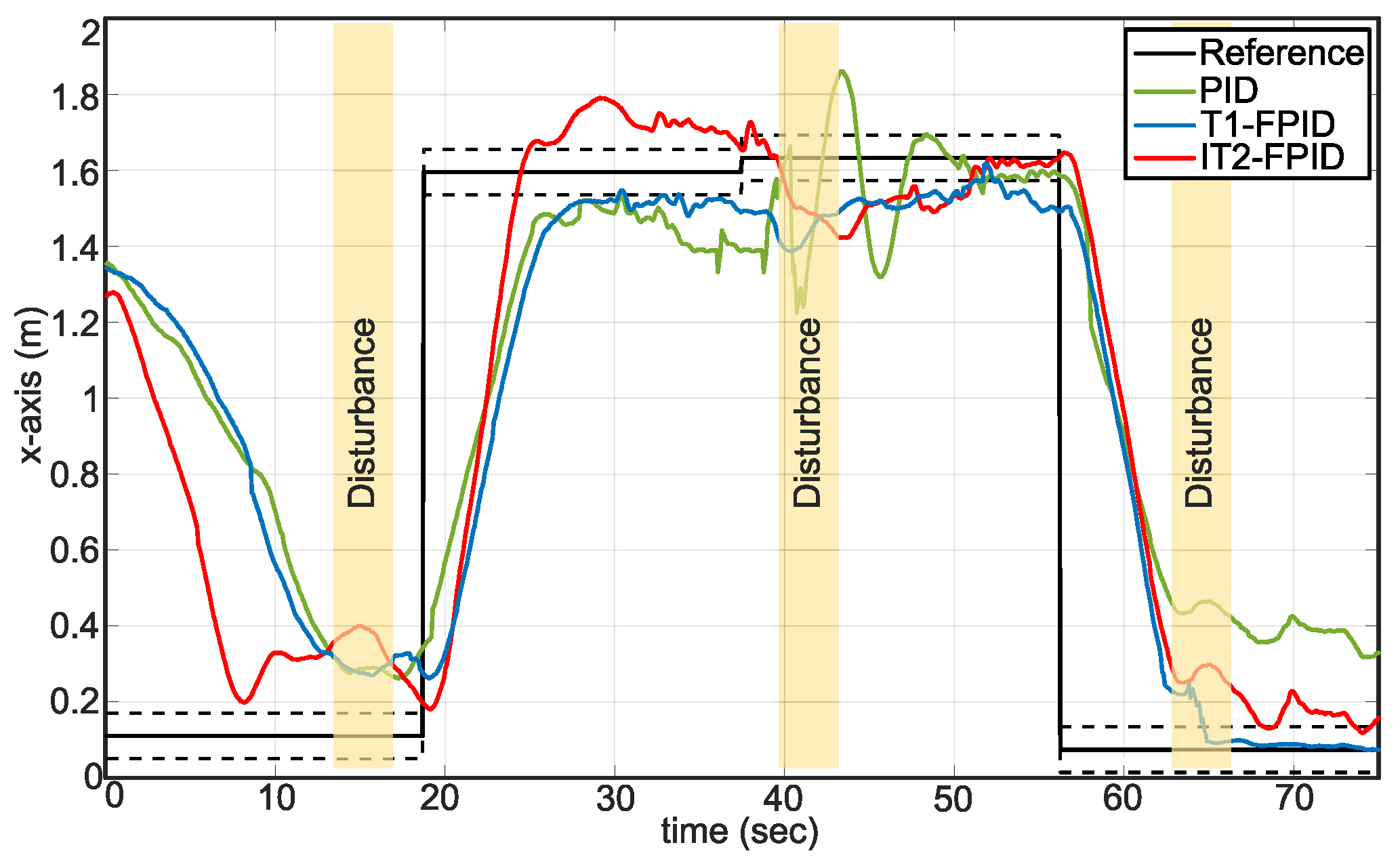
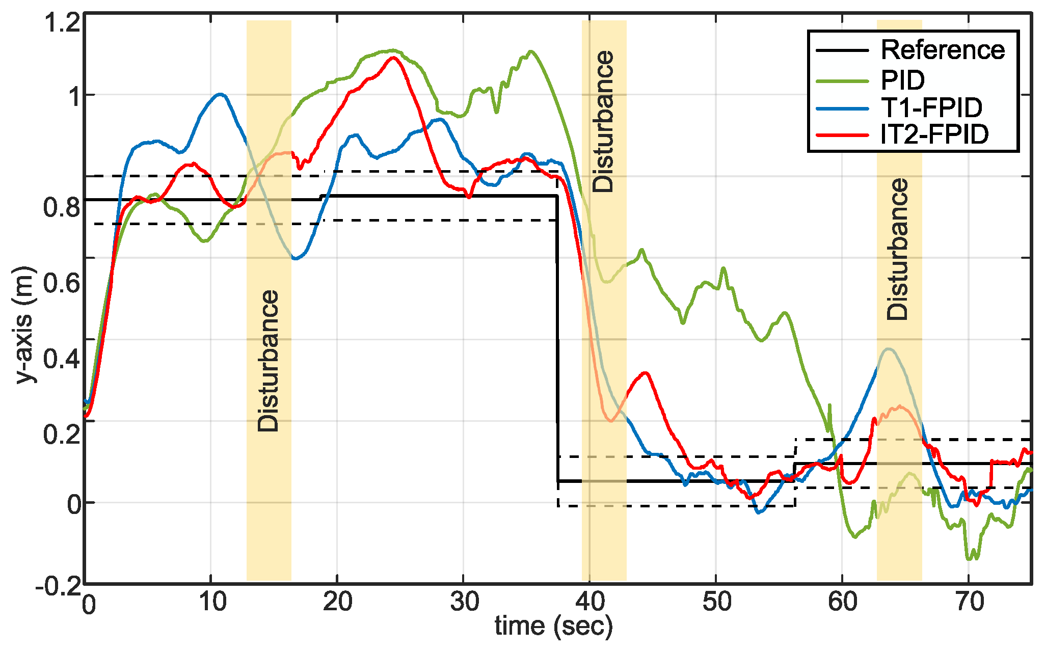
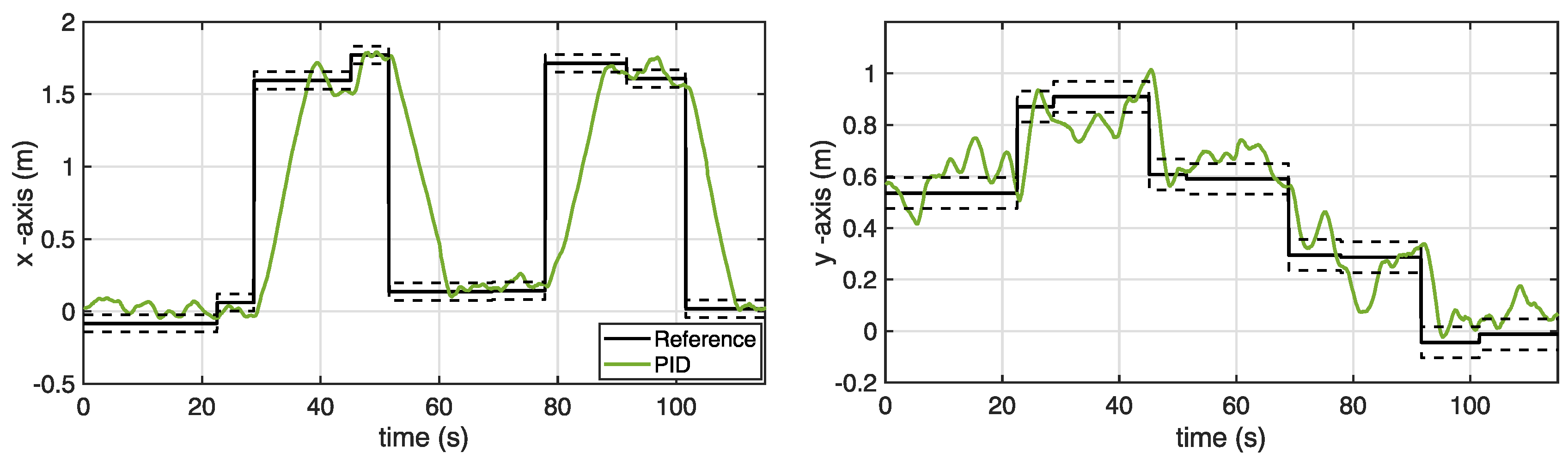
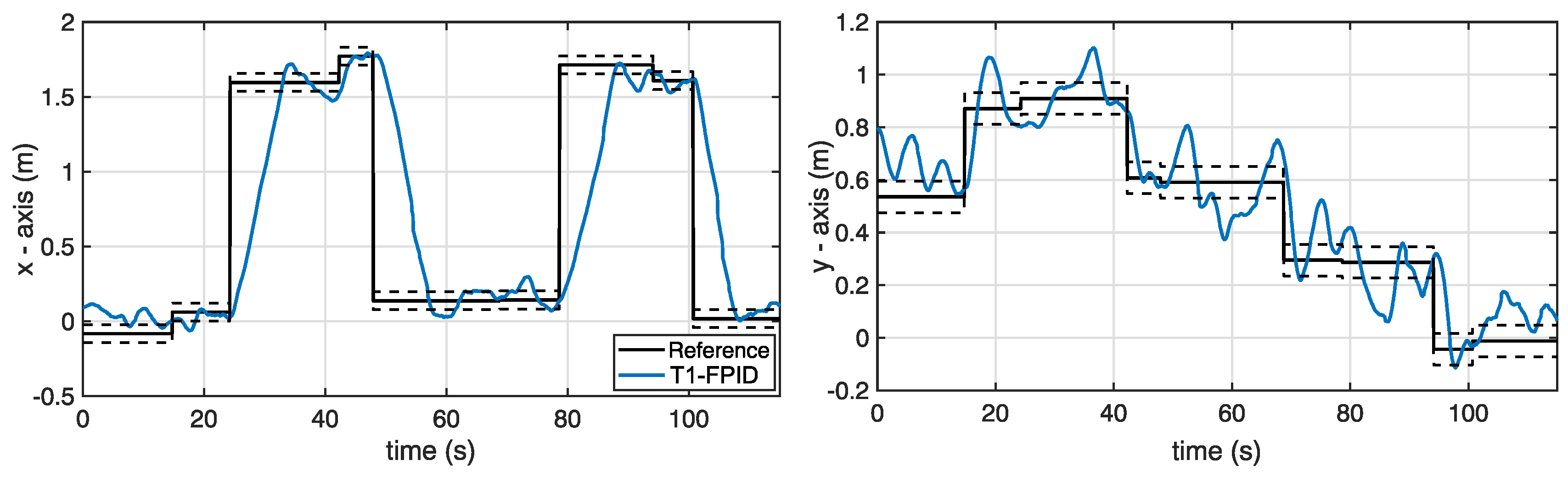
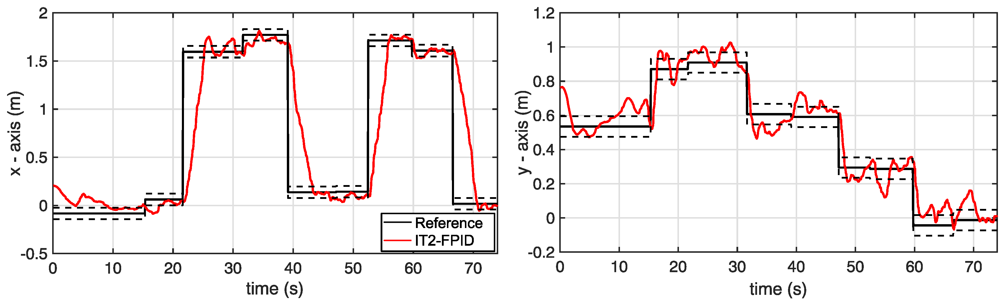
5.2. Set-Point Tracking with Disturbance and the Payload

The results of set-point tracking with disturbance and the payload consist of two different parts. The first relates to payload disturbing, and the second applies to CPP. In this part, all controller structures are tested under disturbance. The payload is disturbed using a stick to implement the disturbances as external disturbances, directly impacting the system stability. After that, in the CPP scenario, the disturbances are generated by themselves as explained in the aforementioned above section.
In Figure 14, the disturbance effects are seen on the x-axis. PID and T1-FPID give slow responses, and generally, they do not reach the reference points. IT2-FPID is not as affected as the others.
In Figure 15, the biggest problem for all controller types is on the y-axis. The PID cannot guarantee stability under disturbance, and T1-FPID and IT2-FPID show a slight overshoot.
After the disturbance-based results, some specific points are given for each controller. The second experiment of the IT2-FPID controller is coverage path planning. Each vertex of the coverage path planning is fixed and determined before the test, and these are given as reference points. The reference point changes to the next vertex when the UAV converges or reaches the current vertex. Considering the task compilation time, IT2-FPID, T1-FPID, and PID complete the task in 74.55 s, 112.35 s, and 120.15 s, respectively. In addition to a faster completion time, IT2-FPID also shows better results in other ways.
The first experiment of the CPP is the PID controller structure for the real-time UAV with a flexible cable-connected payload as shown in Figure 16. PID shows a small steady-state error and slower system response on the x-axis. However, PID has a problem on the y-axis. It does not reach the reference points properly.
In Figure 17, T1-FPID does not show promising results compared with the PID results on the x-axis, but it completes the task time faster than the PID controller; these results are plausible. However, T1-FPID oscillates on the y-axis. This issue can be explained by the fact that the payload is not at the CoM of the UAV but nearer the front side. Therefore, the problem on the y-axis is expected for all of the controller’s structures.
The last and the best results achieved with the IT2-FPID are shown in Figure 18. It completes the CPP task in 74.55 s. In addition, it has a better settling time, oscillation, and steady-state error in terms of minor errors and short time. Although the payload position problem on CoM exists for the other controllers, IT2-FPID overcomes the problem steadfastly.
The experimental results on each axis are analysed separately. RMSE is chosen as a performance index for the comparison of the controllers. In Table 4, the results of RMSE on the x-axis are shown. The best results of each experiment are IT2-FPID on the x-axis.
As far as the RMSE values obtained in the set-point tracking scenario and in the testing against the disturbance, that is, disturbing the payload with a stick, are considered, IT2-FPID shows almost two times better results when compared to PID and T1-FPID as given in Table 5.
In summary, IT2-FPID has the best performance results in all two robustness tests. Considering the aim of the testing for IT2-FPID, the minimum task time, and RMSE values, maximum accuracy is obtained. However, although T1-FPID is not as good as IT2-FPID, it has better results than the compared PID controller. In the simulation, 20 independent tests are conducted, and then 5 independent tests are run in the real-time system.

6. Conclusions and Future Works

In this study, the flexible cable-connected unknown payload, which is a challenging engineering problem, is described. The challenging problems are related to the swinging unknown payloads and point-based reference trajectories. For this challenging engineering problem, a proportional–integral–derivative (PID) controller, type-1 Fuzzy PID controller (T1-FPID), and interval type-2 Fuzzy PID controller (IT2-FPID) are tuned and implemented on a real UAV. The control algorithms are generic and can be applied to different types and sizes of UAVs, although the experiments are performed using a DJI Tello UAV. The performance of the IT2-FPID is also compared against a PID and a T1-FPID controller. After set-point tracking and robustness testing via disturbing the payload with a stick and changing the reference points in coverage path planning (CPP), causing the payload to swing, the experimental results show that the IT2-FPID is better than the controllers. There are different aims for each test, such as minimum task time and RMSE. Disturbing effects of the flexible cable-connected payload on the UAV are shown throughout the experiments. These adverse effects can be eliminated by the three compared controllers to some point, but the results show the superiority of the IT2-FPID. As an example from the experiments, although the PID controller may solve the trajectory-tracking problem, the uncertainties, such as the unknown payload connection via flexible cable and disturbing the payload, lead to highly detrimental results for the PID controller. Thanks to implementing the IT2-FPID controller, these problems are eliminated considerably. Consequently, the system stability is guaranteed without considering the changes in the system dynamics equations and redesigning the controller.
After the controller design, the sensor part of the UAV will be improved to achieve better accuracy. In order to improve the sensor accuracy, the noise distribution will also be investigated, and then the system will be tested both in the simulation environment and in real time. According to the type of distribution, a filter design will be included to eliminate such noise and general disturbances. Lastly, a theoretical analysis of the performance of the proposed approach under internal and external disturbances is a topic of future work.

Supplementary Materials

The following supporting information can be downloaded at: https://www.mdpi.com/article/10.3390/a16060273/s1.

Author Contributions

The authors’ contributions are conceptualization, F.C., O.F.D., L.M. and M.M.; methodology, F.C. and O.F.D.; software, F.C.; validation, F.C. and O.F.D.; formal analysis: all authors; investigation: F.C., L.M., T.K., M.M.; resources: F.C., L.M., M.M. and T.K.; data curation: F.C.; writing original draft preparation: F.C.; writing—review and editing: F.C., L.M., T.K. and M.M.; visualization: F.C.; supervision: L.M. and M.M. All authors have read and agreed to the submitted version of the manuscript.

Funding

This research received no external funding.

Data Availability Statement

Not applicable.

Acknowledgments

We acknowledge the Turkish government for funding the doctoral scholarship of Fethi Candan. T. Kumbasar was supported by the BAGEP Award of the Science Academy and the TUBA GEBIP award from the Turkish Academy of Sciences.

Conflicts of Interest

The authors declare no conflict of interest.

Appendix A. UAV Linear Model

The transformation between the body-fixed frame and the inertial frame is achieved with a rotation matrix R for inverse mapping and a transitional matrix T [8,9,32,51] of the form
R = 1 0 s ( θ ) 0 c ( ϕ ) c ( θ ) s ( ϕ ) 0 s i n ( ϕ ) c o s ( ϕ ) c ( θ ) , T = 1 s ( ϕ ) t ( θ ) c ( ϕ ) t ( θ ) 0 c ( ϕ ) s ( ϕ ) 0 s ( ϕ ) / c ( θ ) c ( ϕ ) / c ( θ ) .
In this study, the heading angle of the UAV—yaw ( ψ )—is fixed and is equal to ψ = 0 . For this reason, the defined rotation matrix form is R = R ϕ R θ .
Unlike the nonlinear model of the UAV, the definition of the linear model is represented with simpler equations. As a consequence, U shows the control input values of the system of Equation (A2):
U = [ F t h r u s t B τ ϕ τ θ τ ψ ] .
Equation (A3) is obtained from the equation corresponding to each U input value:
U = F t h r u s t B τ ϕ τ θ τ ψ = b b b b b l b l b l b l b l b l b l b l d d d d Ω 1 2 Ω 2 2 Ω 3 2 Ω 4 2 .
w ˙ B = I B 1 τ r o t o r B = 1 I x b l τ ϕ / 2 1 I y b l τ θ / 2 1 I z d τ ψ .
In the above equations, Ω i denotes the angular velocity of the UAV propeller, d is the drag coefficient of rotors, and l is the distance between the rotor and CoM. When writing the inertia matrix ( I B ) for each torque, they are defined as inertia tensors ( I x = 0.679 × 10 2 , I y = 0.679 × 10 2 , I z = 1.313 × 10 2 [24,34]).
To linearise the equation above by using the Taylor approximation, the following equation is used:
U i = U i 0 + d U i d Ω i | Ω i 0 ( Ω Ω i 0 ) .
In the equation above, the subscript of ( . ) 0 means the hovering mode condition of the UAV. Therefore, the UAV hovering operation point is given by the following equation:
U 0 = [ m g 0 0 0 ] T , Ω i 0 = m g 4 b .
x ¨ y ¨ z ¨ = g ( s ( ψ 0 ) ϕ + c ( ψ 0 ) θ ) g ( s ( ψ 0 ) θ + c ( ψ 0 ) ϕ ) F t h r u s t B .

Appendix B. Big Bang–Big Crunch Optimisation Method

To find the optimal parameters of the controllers, we use the Big Bang–Big Crunch (BB-BC) optimisation method. The proposed optimisation method has shown a faster response than the global optimisation methods [31]. The BB-BC exists in two primary phases. The “Big Bang phase” involves randomly distributed candidate solutions across the search space, followed by the “Big Crunch phase,” which involves calculating the population’s centre of mass using a contraction procedure. Like other evolutionary search methods, the initial Big Bang population is produced randomly over the search space. Similarly, all following Big Bang phases are randomly distributed around the centre of mass or the best-fitted individual.
In [31,52], the working concept of this evolutionary approach consists of changing a converging result into a chaotic state, which is a new set of solutions. The algorithm starts by generating a random population of candidates for calculating fitness values. Using Equation (A8), the centre of mass is calculated, and the selection is based on either the best individual (fitness value) or the centre of mass. Similar to evolutionary computing (EC) algorithms, a new set of candidates is generated based on the previously selected individual via adding or subtracting a random number whose value changes adaptively. The whole process is then repeated (without the initialisation) if the stopping criterion has not been met.
During the Big Crunch, a contraction method is used after the Big Bang. The contraction operator computes a centre of mass using the current locations of each candidate, resulting in the population and its associated cost function value. The centre of mass x c position may be calculated using the following formula:
x c = i = 1 N 1 f i x i i = 1 N 1 f i .
where x i is the candidate position, and f i is the cost function value for each candidate i and population size N. The new value x i n e w is
x i n e w = x c + σ .
where x i is the new candidate result and σ gives the standard deviation of a standard normal distribution.
For the next iteration Big Bang phase, the new generation is distributed around x c as follows:
σ = r α x m a x x m i n k ,
In Equation (A10), the standard deviation reduces as each repetition progresses. Moreover, r is a random number and α is a parameter bounding the size of the search space and
x i n e w = x c + r α ( x m a x x m i n ) k .
Here, the maximum and minimum limits are given as x m a x and x m i n , respectively. Additionally, k is the number of iterations for the optimisation. While, typically, distributed numbers may exceed ± 1 , the population must be limited to the search space boundaries. Therefore, the candidate results are constrained inside the search space boundaries due to this narrowing.

References

  1. Sun, Z.; Piao, H.; Yang, Z.; Zhao, Y.; Zhan, G.; Zhou, D.; Meng, G.; Chen, H.; Chen, X.; Qu, B.; et al. Multi-agent hierarchical policy gradient for Air Combat Tactics emergence via self-play. Eng. Appl. Artif. Intell. 2021, 98, 104112. [Google Scholar] [CrossRef]
  2. Bellocchio, E.; Crocetti, F.; Costante, G.; Fravolini, M.L.; Valigi, P. A novel vision-based weakly supervised framework for autonomous yield estimation in agricultural applications. Eng. Appl. Artif. Intell. 2022, 109, 104615. [Google Scholar] [CrossRef]
  3. Mohamadi, H.E.; Kara, N.; Lagha, M. Heuristic-driven strategy for boosting aerial photography with multi-UAV-aided Internet-of-Things platforms. Eng. Appl. Artif. Intell. 2022, 112, 104854. [Google Scholar] [CrossRef]
  4. Fu, C.; Ding, F.; Li, Y.; Jin, J.; Feng, C. Learning dynamic regression with automatic distractor repression for real-time UAV tracking. Eng. Appl. Artif. Intell. 2021, 98, 104116. [Google Scholar] [CrossRef]
  5. Luperto, M.; Amigoni, F. Reconstruction and prediction of the layout of indoor environments from two-dimensional metric maps. Eng. Appl. Artif. Intell. 2022, 113, 104910. [Google Scholar] [CrossRef]
  6. Argentim, L.M.; Rezende, W.C.; Santos, P.E.; Aguiar, R.A. PID, LQR and LQR-PID on a quadcopter platform. In Proceedings of the International Conference on Informatics, Electronics and Vision (ICIEV), Dhaka, Bangladesh, 17–18 May 2013; IEEE: Piscataway, NJ, USA, 2013; pp. 1–6. [Google Scholar]
  7. Khan, A.A.; Rapal, N. Fuzzy PID controller: Design, tuning and comparison with conventional PID controller. In Proceedings of the 2006 IEEE International Conference on Engineering of Intelligent Systems, Islamabad, Pakistan, 22–23 April 2006; IEEE: Piscataway, NJ, USA, 2006; pp. 1–6. [Google Scholar]
  8. Candan, F.; Beke, A.; Kumbasar, T. Design and Deployment of Fuzzy PID Controllers to the nano quadcopter Crazyflie 2.0. In Proceedings of the Innovations in Intelligent Systems and Applications (INISTA), Thessaloniki, Greece, 3–5 July 2018; IEEE: Piscataway, NJ, USA, 2018; pp. 1–6. [Google Scholar]
  9. Kaplan, M.R.; Eraslan, A.; Beke, A.; Kumbasar, T. Altitude and position control of parrot mambo minidrone with PID and fuzzy PID controllers. In Proceedings of the 11th International Conference on Electrical and Electronics Engineering (ELECO), Bursa, Turkey, 28–30 November 2019; IEEE: Piscataway, NJ, USA, 2019; pp. 785–789. [Google Scholar]
  10. Noordin, A.; Mohd Basri, M.A.; Mohamed, Z. Real-Time Implementation of an Adaptive PID Controller for the Quadrotor MAV Embedded Flight Control System. Aerospace 2023, 10, 59. [Google Scholar] [CrossRef]
  11. Everett, M.F. LQR with Integral Feedback on a Parrot Minidrone. Mass. Inst. Technol. Tech. Rep. 2015, 1, 1–6. [Google Scholar]
  12. Okasha, M.; Kralev, J.; Islam, M. Design and Experimental Comparison of PID, LQR and MPC Stabilizing Controllers for Parrot Mambo Mini-Drone. Aerospace 2022, 9, 298. [Google Scholar] [CrossRef]
  13. Barzanooni, E.; Salahshoor, K.; Khaki-Sedigh, A. Attitude flight control system design of UAV using LQG\LTR multivariable control with noise and disturbance. In Proceedings of the 3rd RSI International Conference on Robotics and Mechatronics (ICROM), Tehran, Iran, 7–9 October 2015; IEEE: Piscataway, NJ, USA, 2015; pp. 188–193. [Google Scholar]
  14. Zhao, W.; Go, T.H. Quadcopter formation flight control combining MPC and robust feedback linearization. J. Frankl. Inst. 2014, 351, 1335–1355. [Google Scholar] [CrossRef]
  15. Ganga, G.; Dharmana, M.M. MPC controller for trajectory tracking control of quadcopter. In Proceedings of the 2017 International Conference on Circuit, Power and Computing Technologies (ICCPCT), Kollam, India, 20–21 April 2017; IEEE: Piscataway, NJ, USA, 2017; pp. 1–6. [Google Scholar]
  16. Ortiz, J.P.; Minchala, L.I.; Reinoso, M.J. Nonlinear robust H-Infinity PID controller for the multivariable system quadrotor. IEEE Lat. Am. Trans. 2016, 14, 1176–1183. [Google Scholar] [CrossRef]
  17. Hosseinzadeh, M.; Sadati, N.; Zamani, I. H∞disturbance attenuation of fuzzy large-scale systems. In Proceedings of the 2011 IEEE International Conference on Fuzzy Systems (FUZZ-IEEE 2011), Taipei, Taiwan, 27–30 June 2011; IEEE: Piscataway, NJ, USA, 2011; pp. 2364–2368. [Google Scholar]
  18. Wenzel, K.E.; Masselli, A.; Zell, A. Automatic take off, tracking and landing of a miniature UAV on a moving carrier vehicle. J. Intell. Robot. Syst. 2011, 61, 221–238. [Google Scholar] [CrossRef]
  19. Palossi, D.; Singh, J.; Magno, M.; Benini, L. Target following on nano-scale unmanned aerial vehicles. In Proceedings of the 7th IEEE International Workshop on Advances in Sensors and Interfaces (IWASI), Vieste, Italy, 15–16 June 2017; IEEE: Piscataway, NJ, USA, 2017; pp. 170–175. [Google Scholar]
  20. Greiff, M. Modelling and Control of the Crazyflie Quadrotor for Aggressive and Autonomous Flight by Optical Flow Driven State Estimation. Master’s Thesis, Lund University, Department of Automatic Control, Sweden, Switzerland, 2017. [Google Scholar]
  21. Souza, R.M.J.A.; Lima, G.V.; Morais, A.S.; Oliveira-Lopes, L.C.; Ramos, D.C.; Tofoli, F.L. Modified artificial potential field for the path planning of aircraft swarms in three-dimensional environments. Sensors 2022, 22, 1558. [Google Scholar] [CrossRef] [PubMed]
  22. Nguyen, N.P.; Lee, B.H.; Xuan-Mung, N.; Ha, L.N.N.T.; Jeong, H.S.; Lee, S.T.; Hong, S.K. Persistent Charging System for Crazyflie Platform. Drones 2022, 6, 212. [Google Scholar] [CrossRef]
  23. Belkhale, S.; Li, R.; Kahn, G.; McAllister, R.; Calandra, R.; Levine, S. Model-based meta-reinforcement learning for flight with suspended payloads. IEEE Robot. Autom. Lett. 2021, 6, 1471–1478. [Google Scholar] [CrossRef]
  24. Rao, J.; Li, B.; Zhang, Z.; Chen, D.; Giernacki, W. Position control of quadrotor uav based on cascade fuzzy neural network. Energies 2022, 15, 1763. [Google Scholar] [CrossRef]
  25. Lee, D.; Park, W.; Nam, W. Autonomous Landing of Micro Unmanned Aerial Vehicles with Landing-Assistive Platform and Robust Spherical Object Detection. Appl. Sci. 2021, 11, 8555. [Google Scholar] [CrossRef]
  26. Islam, S.; Liu, P.X.; El Saddik, A. Robust control of four-rotor unmanned aerial vehicle with disturbance uncertainty. IEEE Trans. Ind. Electron. 2014, 62, 1563–1571. [Google Scholar] [CrossRef]
  27. Qian, L.; Liu, H.H. Path-following control of a quadrotor UAV with a cable-suspended payload under wind disturbances. IEEE Trans. Ind. Electron. 2019, 67, 2021–2029. [Google Scholar] [CrossRef]
  28. Guo, K.; Jia, J.; Yu, X.; Guo, L.; Xie, L. Multiple observers based anti-disturbance control for a quadrotor UAV against payload and wind disturbances. Control Eng. Pract. 2020, 102, 104560. [Google Scholar] [CrossRef]
  29. Quintero, S.A.; Hespanha, J.P. Vision-based target tracking with a small UAV: Optimization-based control strategies. Control Eng. Pract. 2014, 32, 28–42. [Google Scholar] [CrossRef]
  30. Shakeel, T.; Arshad, J.; Jaffery, M.H.; Rehman, A.U.; Eldin, E.T.; Ghamry, N.A.; Shafiq, M. A Comparative Study of Control Methods for X3D Quadrotor Feedback Trajectory Control. Appl. Sci. 2022, 12, 9254. [Google Scholar] [CrossRef]
  31. Erol, O.K.; Eksin, I. A new optimization method: Big bang–big crunch. Adv. Eng. Softw. 2006, 37, 106–111. [Google Scholar] [CrossRef]
  32. Abdelmoeti, S.; Carloni, R. Robust control of UAVs using the parameter space approach. In Proceedings of the IEEE/RSJ International Conference on Intelligent Robots and Systems (IROS), Daejeon, Republic of Korea, 9–14 October 2016; IEEE: Piscataway, NJ, USA, 2016; pp. 5632–5637. [Google Scholar]
  33. DJI Tello, C. DJI Tello EDU, Ryzerobotics. Available online: https://www.ryzerobotics.com/tello-edu (accessed on 16 June 2022).
  34. Giernacki, W.; Rao, J.; Sladic, S.; Bondyra, A.; Retinger, M.; Espinoza-Fraire, T. DJI Tello Quadrotor as a Platform for Research and Education in Mobile Robotics and Control Engineering. In Proceedings of the 2022 International Conference on Unmanned Aircraft Systems (ICUAS), Dubrovnik, Croatia, 21–24 June 2022; IEEE: Piscataway, NJ, USA, 2022; pp. 735–744. [Google Scholar]
  35. Sarabakha, A.; Fu, C.; Kayacan, E.; Kumbasar, T. Type-2 fuzzy logic controllers made even simpler: From design to deployment for UAVs. IEEE Trans. Ind. Electron. 2017, 65, 5069–5077. [Google Scholar] [CrossRef]
  36. Sakalli, A.; Kumbasar, T.; Mendel, J.M. Towards systematic design of general type-2 fuzzy logic controllers: Analysis, interpretation, and tuning. IEEE Trans. Fuzzy Syst. 2020, 29, 226–239. [Google Scholar] [CrossRef]
  37. Lee, D.H.; Park, D. An efficient algorithm for fuzzy weighted average. Fuzzy Sets Syst. 1997, 87, 39–45. [Google Scholar] [CrossRef]
  38. Chang, P.T.; Hung, K.C.; Lin, K.P.; Chang, C.H. A comparison of discrete algorithms for fuzzy weighted average. IEEE Trans. Fuzzy Syst. 2006, 14, 663–675. [Google Scholar] [CrossRef]
  39. Palma, L.B.; Antunes, R.A.; Gil, P.; Brito, V. Takagi-Sugeno-Kang fuzzy PID control for DC electrical machines. In Proceedings of the 2020 IEEE 14th International Conference on Compatibility, Power Electronics and Power Engineering (CPE-POWERENG), Setubal, Portugal, 8–10 July 2020; IEEE: Piscataway, NJ, USA, 2020; Volume 1, pp. 309–316. [Google Scholar]
  40. Biglarbegian, M.; Melek, W.W.; Mendel, J.M. Design of novel interval type-2 fuzzy controllers for modular and reconfigurable robots: Theory and experiments. IEEE Trans. Ind. Electron. 2010, 58, 1371–1384. [Google Scholar] [CrossRef]
  41. Kavikumar, R.; Sakthivel, R.; Kwon, O.M.; Selvaraj, P. Robust tracking control design for fractional-order interval type-2 fuzzy systems. Nonlinear Dyn. 2022, 107, 3611–3628. [Google Scholar] [CrossRef]
  42. Firouzi, B.; Alattas, K.A.; Bakouri, M.; Alanazi, A.K.; Mohammadzadeh, A.; Mobayen, S.; Fekih, A. A Type-2 Fuzzy Controller for Floating Tension-Leg Platforms in Wind Turbines. Energies 2022, 15, 1705. [Google Scholar] [CrossRef]
  43. Tai, K.; El-Sayed, A.R.; Biglarbegian, M.; Gonzalez, C.I.; Castillo, O.; Mahmud, S. Review of recent type-2 fuzzy controller applications. Algorithms 2016, 9, 39. [Google Scholar] [CrossRef]
  44. Mathworks, C. Computer Vision Toolbox for Matlab, Matlab. Available online: https://uk.mathworks.com/help/vision/index.html (accessed on 16 June 2022).
  45. Python.org. Python3. Available online: https://www.python.org/ (accessed on 14 January 2023).
  46. Torres, M.; Pelta, D.A.; Verdegay, J.L.; Torres, J.C. Coverage path planning with unmanned aerial vehicles for 3D terrain reconstruction. Expert Syst. Appl. 2016, 55, 441–451. [Google Scholar] [CrossRef]
  47. Cabreira, T.M.; Brisolara, L.B.; Ferreira, P.R., Jr. Survey on coverage path planning with unmanned aerial vehicles. Drones 2019, 3. [Google Scholar] [CrossRef]
  48. Galceran, E.; Carreras, M. A survey on coverage path planning for robotics. Robot. Auton. Syst. 2013, 61, 1258–1276. [Google Scholar] [CrossRef]
  49. Intel Realsense. Intel Realsense D415. Available online: https://www.intelrealsense.com/depth-camera-d415 (accessed on 16 June 2022).
  50. Santos, M.C.; Santana, L.V.; Brandão, A.S.; Sarcinelli-Filho, M.; Carelli, R. Indoor low-cost localization system for controlling aerial robots. Control Eng. Pract. 2017, 61, 93–111. [Google Scholar] [CrossRef]
  51. Castillo, P.; Lozano, R.; Dzul, A. Stabilization of a mini-rotorcraft having four rotors. In Proceedings of the 2004 IEEE/RSJ International Conference on Intelligent Robots and Systems (IROS) (IEEE Cat. No. 04CH37566), Sendai, Japan, 28 September–2 October 2004; IEEE: Piscataway, NJ, USA, 2004; Volume 3, pp. 2693–2698. [Google Scholar]
  52. Upasane, S.J.; Hagras, H.; Anisi, M.H.; Savill, S.; Taylor, I.; Manousakis, K. A Big Bang-Big Crunch Type-2 Fuzzy Logic System for Explainable Predictive Maintenance. In Proceedings of the 2021 IEEE International Conference on Fuzzy Systems (FUZZ-IEEE), Luxembourg, 11–14 July 2021; IEEE: Piscataway, NJ, USA, 2021; pp. 1–8. [Google Scholar]
Figure 1. The DJI Tello UAV used in the implementation [33].
Algorithms 16 00273 g001
Figure 2. DJI Tello and payload connection.
Algorithms 16 00273 g002
Figure 3. Illustration of the T1- and IT2-FPID controller.
Algorithms 16 00273 g003
Figure 4. Illustrated T1 fuzzy MFs and control surface.
Algorithms 16 00273 g004
Figure 5. Interval type-2 fuzzy MFs and control surface.
Algorithms 16 00273 g005
Figure 6. The control surface differences between T1-FPID and IT2-FPID.
Algorithms 16 00273 g006
Figure 7. Testing results of the compared controllers in the simulation.
Algorithms 16 00273 g007
Figure 8. Fuzzy logic-based position control system.
Algorithms 16 00273 g008
Figure 9. Camera trigonometric formation scheme and the UAV position.
Algorithms 16 00273 g009
Figure 10. Example of coverage path planning.
Algorithms 16 00273 g010
Figure 11. Coverage path planning for the UAV.
Algorithms 16 00273 g011
Figure 12. Set-point tracking results on the x-axis.
Algorithms 16 00273 g012
Figure 13. Set-point tracking results on the y-axis.
Algorithms 16 00273 g013
Figure 14. Disturbance results on the x-axis.
Algorithms 16 00273 g014
Figure 15. Disturbance results on the y-axis.
Algorithms 16 00273 g015
Figure 16. Coverage path planning with PID.
Algorithms 16 00273 g016
Figure 17. Coverage path planning with T1-FPID.
Algorithms 16 00273 g017
Figure 18. Coverage path planning with IT2-FPID.
Algorithms 16 00273 g018
Table 1. The rule table of T1- and IT2-FPID controller.
E / Δ E PZN
PPB:1PM:0.65Z:0
ZPM:0.65Z:0NM:−0.65
NZ:0NM:−0.65NB:−1
Table 2. Tuned parameters and their performance criteria results.
ControllerParametersISE
PID K c = 0.0472 , T i = 0.0052 , T d = 0.0445 82,133.4
T1-FPID K e = 0.019 , K d = 0.0019 , K 0 = 0.0001 , K 1 = 30 55,128.2
IT2-FPID K e = 0.019 , K d = 0.0019 , K 0 = 0.0001 , K 1 = 30 , ( α = 0.25 , ζ = 0.5 ) 36,371.9
: These parameters have been selected before BB-BC.
Table 3. Camera HSV parameters.
HSVHueSaturationValue
Maximum Values160600
Minimum Values200255255
Table 4. RMSE values on x-axis.
RMSE Values (m)PIDT1-FPIDIT2-FPID
Set-Point Tracking0.22750.22550.2218
Under Disturbance0.55740.54900.4971
CPP Results0.57190.55970.4540
Table 5. RMSE values on y-axis.
RMSE Values (m)PIDT1-FPIDIT2-FPID
Set-Point Tracking0.1370.09640.0805
Under Disturbance0.31030.18770.1810
CPP Results0.13380.12980.1068
Disclaimer/Publisher’s Note: The statements, opinions and data contained in all publications are solely those of the individual author(s) and contributor(s) and not of MDPI and/or the editor(s). MDPI and/or the editor(s) disclaim responsibility for any injury to people or property resulting from any ideas, methods, instructions or products referred to in the content.

