Optimal Siting and Sizing of FACTS in Distribution Networks Using the Black Widow Algorithm

Abstract

The problem regarding the optimal placement and sizing of different FACTS (flexible alternating current transmission systems) in electrical distribution networks is addressed in this research by applying a master–slave optimization approach. The FACTS analyzed correspond to the unified power flow controller (UPFC), the thyristor-controlled shunt compensator (TCSC, also known as the thyristor switched capacitor, or TSC), and the static var compensator (SVC). The master stage is entrusted with defining the location and size of each FACTS device using hybrid discrete-continuous codification through the application of the black widow optimization (BWO) approach. The slave stage corresponds to the successive approximations power flow method based on the admittance grid formulation, which allows determining the expected costs of the energy losses for a one-year operation period. The numerical results in the IEEE 33-, 69-, and 85-bus grids demonstrate that the best FACTS device for locating in distribution networks is the SVC, given that, when compared to the UPFC and the TCSC, it allows for the best possible reduction in the equivalent annual investment and operating cost. A comparative analysis with the General Algebraic Modeling System software, with the aim to solve the exact mixed-integer nonlinear programming model, demonstrated the proposed BWO approach’s effectiveness in determining the best location and size for the FACTS in radial distribution networks. Reductions of about $12.63\%$ and $13.97\%$ concerning the benchmark cases confirmed that the SVC is the best option for reactive power compensation in distribution grids.

1. Introduction

1.1. General Context

The electrical power system comprises the generation, transmission, and distribution phases. In the distribution stage, the electrical energy finally reaches the consumer at medium- and low-voltage levels [1]. Given the voltage levels, distribution networks take up hundreds of kilometers in urban and rural grids, which implies that maintaining a high-quality level during their operation is a difficult task for distribution companies [2]. One of the key factors for distribution networks corresponds to the possibility of extending the electrical service to new potential end users while ensuring low power levels [3,4]. In the Colombian context, medium- and low-voltage distribution grids can have energy losses between $14.5\%$ and $21.8\%$ [5]. However, regulatory entities only recognize distribution companies through their energy pricing for an end-user transfer as a maximum $8\%$ of the total energy losses costs, which implies that improving the efficiency of distribution systems is a pending task for Colombian distribution companies [6].

1.2. Motivation

Energy losses in distribution networks are high in comparison with transmission systems, as distribution grids operating at medium- and low-voltage levels are constructed considering a radial topology (a connected tree with only one path between the substation and each load node) [7]. These grids are built with a radial structure to reduce investment costs and the complexities of coordinating protection devices [8]. To minimize energy loss indices in radial distribution networks, the following strategies are typically employed: (i) optimal grid reconfiguration using available tie-lines [9]; (ii) the optimal placement of dispersed generators and energy storage systems [10,11], and (iii) the optimal siting and sizing of shunt reactive power compensators [12]. This research aims at reducing the expected energy losses costs by proposing the efficient integration of FACTS (flexible alternating current transmission systems) devices in the grid. The FACTS analyzed correspond to the unified power flow controller (UPFC), the thyristor-controlled shunt compensator (TCSC), and the static var compensator (SVC) [13].

The main idea of integrating FACTS in distribution networks is to determine the expected reductions that can be reached with different shunt reactive power compensators based on power electronic interfaces regarding energy loss reductions. This is an alternative to classical fixed-step capacitor banks [14]. Therefore, in this research, our efforts are focused on locating and sizing UPFCs, TCSCs, and SVCs in distribution networks with radial or meshed topologies, because the current literature mainly deals with SVCs (or distribution static compensators, D-STATCOMs) [15,16] and conventional fixed-step capacitor banks [17].

1.3. Literature Review

With the advancements made in power electronics, different devices have been created to maximize the use of existing transmission and distribution networks, as is the case of FACTS devices. These not only allow increasing the changeability of the circuits but also reducing losses, regulating voltage values, and improving the power quality and stability of the system [18]. Several authors have focused on establishing different models that enhance the performance of distribution networks via shunt reactive power compensators. The authors of [19] proposed a particle swarm optimization model to determine the optimal location of various types of controlled FACTS devices and thus increase the power transmission capacity of the lines. The study included selecting the optimal device among three options (UPFC, TCSC, and SVC), as well as their location and selection of parameters. The article aimed to maximize the cost–benefit, increase grid loadability, and reduce power losses. The IEEE 30-bus grid was used to evaluate the effectiveness of this optimization approach. The location and configuration of FACTS devices by means of the cross-entropy method were presented in [20]. The main idea of integrating FACTS into power systems is to reduce congestion and line losses by minimizing the number of devices used. A simulation of a 30-node IEEE test system was performed through the implementation of an optimal power solution that considered an economic objective function.

In [21], the moth flame optimization algorithm was implemented to solve the optimal power flow in power grids by including FACTS in the existing infrastructure. The objective of this solution is achieving the reduction in the grid power losses and keeping the voltage levels stable. Variable control was carried out by controlling the reactive power of the generator, configuring the TAPs in the transformers, and setting the parameters of the FACTS. Numerical validations were carried out in the IEEE 57-node test system using SVCs, TCSCs, and thyristor-controlled phase angle regulators. In [22], the maximization of the power system’s loadability was sought through the optimal location of FACTS devices. For this case, TCSC and UPFC devices were used. The improved moth flame optimization method was implemented to obtain the maximum objective function values, and numerical simulations were implemented in the IEEE 30-bus system. It is worth noting that this study aimed to maximize the loadability of the power system, reduce power losses, and minimize voltage variations.

A new multi-objective optimization algorithm was proposed in [13], known as a multi-objective multiverse optimizer, which is employed to determine the location of FACTS in the power system. Thus, it is possible to establish the optimal configurations of the FACTS in order to improve the voltage profiles and reduce power losses. Numerical validations were performed in the IEEE 57-node test system.

In the case of medium-voltage distribution networks, some of the applications regarding FACTS are associated with the optimal integration of distribution static compensations (D-STATCOMs), which essentially correspond to the use of SVC technology with regard to voltage distribution levels [23]. The authors of [24] proposed the optimal integration of D-STATCOMs in radial distribution networks to minimize the expected annual costs of energy losses while considering the investments associated with reactive power compensators. The IEEE 33- and IEEE 69-bus grids were employed as test systems. The resulting mixed-integer nonlinear programming (MINLP) model was solved by implementing the discrete-continuous version of the vortex search algorithm. Numerical results improved the values reached with some exact MINLP solvers available in the General Algebraic Modeling System (GAMS) software.

In [25], the discrete-continuous version of the vortex search algorithm was implemented to define the optimal location and sizing of D-STATCOMs in radial distribution networks. Numerical results in the IEEE 33- and IEEE 69-bus grids showed an efficient numerical performance regarding processing times in comparison with the vortex search algorithm. Additional works regarding the optimal placement of FACTS in electrical distribution networks include sensitivity factors based on stability and power losses indices [26], genetic algorithms [27], and convex approximations [16], among others. Note that the main feature of these works is the use of an economic objective function that seeks to minimize the expected energy loss costs, including the investments made in reactive power compensators.

1.4. Contributions and Scope

Considering the above-presented review of the state of the art, this research makes the following contributions:

i.

The efficient integration of multiple FACTS into radial distribution networks, i.e., UPFC, SVC, and TCSC, applying the black widow optimization algorithm (BWO) and using discrete-continuous codification.

ii.

A validation of the effectiveness of the proposed BWO while considering the existing literature reports regarding the optimal placement and sizing of D-STATCOMs (modeled as an SVC device).

It is worth mentioning that in this research, all the FACTS considered are modeled using cubic functions that represent the investment costs, as reported in [28]. In addition, the multi-period power flow approach based on successive approximations is implemented within the framework of a master–slave strategy, in order to quantify the expected energy loss costs. The BWO approach is the master stage, entrusted with defining the optimal location and size of the FACTS devices, which is then evaluated via the successive approximations power flow (SAPF) method. Regarding the UPFC, it is essential to mention that this research only uses it for managing the reactive power injected into the connected node, as its series component cannot control the active power flow in the distribution branch. This is due to the radial structure of the distribution grid, where the active power flow is only necessary to support the load consumptions downstream of the node and branch where the UPFC is installed.

The selection of the master–slave approach, which is based on the hybridization of the BWO (master stage) and the SAPF (slave stage) for dealing with the exact MINLP model associated with the location and sizing of FACTS devices in distribution networks, was based on the fact that the MINLP problem can be easily decoupled into two sub-problems, i.e., the binary (integer) problem and the continuous problem. The solution of the integer component of the model is easily reached with combinatorial optimization methods (such as the BWO approach), and the continuous part can be efficiently solved with numerical methods applicable to the power flow problem in distribution networks (i.e., the SAPF approach).

Note that the BWO approach is selected in this research as the master optimization method, as it has been proven to be an excellent population-based optimization technique to deal with continuous and integer optimization problems in the current literature [29]. This algorithm can be easily implemented, and its efficiency lies in its similarities with classical genetic optimization algorithms regarding its evolution rules [30]. In addition, after a complete review of the state of the art regarding the location and sizing of FACTS in distribution networks, no evidence for the application of the BWO and its hybridization with the SAPF was found, which constitutes a clear research opportunity.

1.5. Structure of the Document

The remainder of this research is structured as follows. Section 2 presents the exact MINLP formulation regarding the optimal placement and sizing of FACTS in electrical distribution networks. Section 3 describes the main aspects of the proposed solution methodology based on the hybridization of the BWO with the SAPF using a master–slave optimization strategy. Section 4 shows the main characteristics of the test feeders, i.e., the IEEE 33- and 69-bus grids with radial configuration, including the active and reactive power curves and the parameters required for evaluating the objective function. Section 5 presents the numerical validations of the proposed BWO approach to the efficient location and sizing of FACTS in radial distribution networks while performing a comparative analysis with the existing literature reports. Finally, Section 6 lists the conclusions obtained from this research and some possible future developments.

2. Mathematical Formulation

The problem regarding the optimal integration of shunt reactive power compensators in medium-voltage distribution networks involves the minimization of the expected annual grid operating costs associated with the energy losses and the investments made in compensation devices. The main characteristic of the problem is a mixed-integer nonlinear programming (MINLP) structure. The binary/integer part fits the variables associated with the nodes where the compensator devices must be installed. The continuous component of the model refers to the power generation inputs and the voltage magnitudes and angles, as well as the sizes of the reactive power compensators, among others. The general MINLP formulation of the studied problem is detailed below.

2.1. Objective Function Formulation

The main idea of integrating reactive power compensators in distribution networks is to minimize the annual equivalent operating costs, corresponding to the sum of the expected yearly costs of energy losses and the investment made in reactive power compensators. The expected annual operating costs associated with the energy losses are defined in Equation (1) [25].

$$\begin{array}{c}\hfill z_1=C_{kWh}T\sum _{h\in \mathcal{H}}\sum _{k\in \mathcal{N}}\sum _{m\in \mathcal{N}}{Y}_{km}{v}_{kh}{v}_{mh}cos\left({\delta }_{kh}-{\delta }_{mh}-{\theta }_{km}\right)\mathsf{\Delta }h,\end{array}$$

(1)

where $z_1$ defines the objective function value regarding the annual grid power losses costs; $C_{kWh}$ corresponds to the average energy losses costs; T is the number of days in a year; $Y_{km}$ is an element of the admittance matrix associated with the connection of the nodes k and m; $v_{kh}$ defines the voltage magnitude at node k in the period h; $v_{kh}$ defines the voltage magnitude at node m in the period h; ${\delta }_{kh}$ is the variable associated with the voltage angle at node k in the period h; ${\delta }_{mh}$ is the variable associated with the angle of the voltage at node k in the period h; ${\theta }_{km}$ is a parameter associated with the angle of the impedance that relates nodes k and m; and ${\mathsf{\Delta }}_h$ is a parameter associated with the number of periods in the daily analysis, typically defined as an hour or fractions of it. In addition, $\mathcal{N}$ is the set containing all network nodes, and $\mathcal{H}$ is the set associated with the number of periods considered in the daily analysis period.

Note that the objective function in (1) is the classical representation of the expected power losses in all transmission/distribution lines, as a function of the nodal admittance matrix, the voltage profiles, and the cosine function of the voltage and admittance angles [25]. These power losses are summarized for the daily operation scenario under analysis. With this information, the annual expected costs are also calculated, using the average energy cost rate and the number of days in an ordinary year.

Equation (2) defines the investment costs regarding the reactive power compensators, which is modeled as a cubic function, as reported by the authors of [28]. The distinctive characteristic of the objective function (2) is its mathematical structure, i.e., it is a non-convex cubic function. However, the main idea of this function structure is to consider a linear component associated with the investment costs per capacity, in addition to the fact that the quadratic and cubic terms are related to the variable reactive power production costs, which can involve factors regarding the maintenance and degradation of the FACTS devices during their useful life.

$$z_2=T\left(\frac{k_1}{k_2}\right)\sum _{k\in \mathcal{N}}\left({\omega }_1{\left(q_k^{\mathrm{comp}}\right)}^2+{\omega }_2{q}_k^{\mathrm{comp}}+{\omega }_3\right)q_k^{\mathrm{comp}},$$

(2)

where $z_2$ defines the objective function value regarding the investment costs of the shunt power compensators; $k_1$ and $k_2$ are positive constant parameters associated with the annualization of the investment costs of the shunt compensators while considering a planning period of 10 years [27]; $q_k^{\mathrm{comp}}$ is the nominal size of the shunt reactive power compensator located at node k; and ${\omega }_1$, ${\omega }_2$, and ${\omega }_3$ are the cubic, quadratic, and linear coefficients regarding the investment costs of the shunt reactive power compensators.

Note that $z_1$ and $z_2$ are defined as the objective function for the problem regarding the optimal siting and sizing of FACTS in electrical distribution networks, i.e., the sum of the investment and operating costs in $z_{\cos \mathrm{t}}$, as presented in Equation (3) [16].

$$min{z}_{\cos \mathrm{t}}=z_1+z_2,$$

(3)

Remark 1.

The main characteristic of the objective function in (3) is that each one of its components (i.e., $z_1$ and $z_2$) are non-convex objective functions due to the presence of trigonometric and cubic functions. In order for them to be minimized, they require efficient optimization methodologies that deal with nonlinear non-convex function spaces.

2.2. Set of Constraints

The constraints associated with the problem under study include active and reactive power balance, voltage regulation bounds, and limitations regarding the reactive power injected with the FACTS, among others. The set of considered constraints is listed from (4) to (9).

Equations (4) and (5) represent the active and reactive power equilibrium per node and period of time, which are obtained after combining Kirchhoff’s first and second laws while using Tellegen’s theorem [25].

$$p_{kh}^g-P_{kh}^d=\sum _{kϵ\mathcal{N}}\sum _{mϵ\mathcal{N}}{Y}_{km}{v}_{kh}{v}_{mh}cos\left({\delta }_{kh}-{\delta }_{mh}-{\theta }_{km}\right),\left\{\forall k\in \mathcal{N},h\in \mathcal{H}\right\},$$

(4)

$$q_{kh}^g+q_{kh}^{\mathrm{comp}}-Q_{kh}^d=\sum _{kϵ\mathcal{N}}\sum _{mϵ\mathcal{N}}{Y}_{km}{v}_{kh}{v}_{mh}sin\left({\delta }_{kh}-{\delta }_{mh}-{\theta }_{km}\right),\left\{\forall k\in \mathcal{N},h\in \mathcal{H}\right\},$$

(5)

where $p_{kh}^g$ and $P_{kh}^d$ represent the active power generation and the power demanded at k in the period h; $q_{kh}^g$ corresponds to the reactive power generation at node k in the period h; $q_{kh}^{\mathrm{comp}}$ represents the reactive power injection in the FACTS device connected at node k and time h; and $Q_{kh}^d$ denotes the reactive power consumed at node k in the period h.

The box-type constraint defined in (6) is known as the voltage regulation constraint in the specialized literature, and it is typically imposed by regulatory entities in order to ensure a service of good quality for all end users connected to the electrical system [31].

$$V_{min}\le v_{kh}\le V_{max},\left\{\forall k\in \mathcal{N},h\in \mathcal{H}\right\},$$

(6)

where $V_{min}$ and $V_{min}$ are the minimum and maximum voltage limits that can be assigned to the variable $v_{kh}$ for each node and period.

To adequately integrate compensation devices into distribution networks, it is necessary to define their nominal operating sizes within the typical ranges available. At medium-voltage levels, distribution grids are typically designed to supply between 3 and 10 MVA. The sizes of the FACTS are limited by the box-type constraint (7) [16].

$$y_k{Q}_{min}^{\mathrm{comp}}\le q_k^{\mathrm{comp}}\le y_k{Q}_{max}^{\mathrm{comp}},\left\{\forall k\in \mathcal{N}\right\},$$

(7)

where $y_k$ is a binary variable that defines the location ($y_k=1$) or not ($y_k=0$) of a shunt reactive power compensator at node k; and $Q_{min}^{\mathrm{comp}}$ and $Q_{max}^{\mathrm{comp}}$ represent the minimum and maximum sizes allowed for the FACTS devices in the distribution network, which are typically between 0 and 2000 kvar [25].

Once the nominal sizes of the FACTS devices are defined, the next step in their optimal operation is defining the power injection for each period of time. This box-type constraint is defined in (8) [32]. In addition, the amount of FACTS devices available for installation is defined in (9) [25].

$$-q_k^{\mathrm{comp}}\le q_{kh}^{\mathrm{comp}}\le q_k^{\mathrm{comp}},\left\{\forall k\in \mathcal{N},h\in \mathcal{H}\right\},$$

(8)

$$\sum _{k\in \mathbb{N}}{y}_k\le N_A^{\mathrm{comp}},$$

(9)

where $N_A^{\mathrm{comp}}$ is a constant parameter that defines the number of FACTS available for installation in the distribution network.

2.3. Model Interpretation and Characterization

The general MINLP model defined from (1) to (9) can be interpreted as follows:

i.

The first component of the objective function, defined in (1), is associated with the annualized expected costs of energy losses in all the branches of the distribution network. The second component of the objective function, presented in Equation (2), quantifies the expected investment in FACTS to be installed. In addition, the sum of both components defines the objective function studied in this research, as presented in Equation (3).

ii.

Equation (4) and Equation (5) correspond to the power equilibrium restrictions per node and period. These are nonlinear and non-convex constraints whose solution requires the implementation of a numerical method.

iii.

The voltage regulation constraint is defined in Equation (6). This is one of the most typical operating conditions for electrical networks, as it is imposed by regulatory entities at any voltage level in order to ensure the quality of the voltage service for all end users [33].

iv.

Equation (7) is a binary constraint that defines whether a FACTS device will be installed at a particular node k. If $y_k=1$, the compensation device is sized; otherwise, its size must be zero. Box-type constraint (8) sets the daily dispatch of a FACTS device connected at node k by defining the reactive power injection per period. In addition, inequality constraint (9) defines the maximum number of compensation devices available for installation in the distribution network under analysis.

Remark 2.

Given the complexity of the optimization model (1)–(9) (i.e., the nonlinearities and non-convexities of the objective function and the power balance constraints), and as recommended by the authors of [25], one of the most suitable optimization approaches is the hybridization of a combinatorial optimizer with an efficient power flow approach within a master–slave programming structure.

To illustrate the complexity of the exact MINLP model defined in (1)–(9),

Table 1. Number of variables and equations that make up the MINLP model under analysis.

Equations	Type	Number
Energy losses costs (Equation (1))	Equality	1
Investment costs of FACTS devices (Equation (2))	Equality	1
Objective function (Equation (3))	Equality	1
Active power balance (Equation (4))	Equality	$nh$
Reactive power balance (Equation (5))	Equality	$nh$
Voltage regulation (Equation (6))	Inequality	$nh$
FACTS nominal size (Equation (7))	Inequality	n
FACTS daily operation (Equation (8))	Inequality	$nh$
FACTS availability (Equation (9))	Inequality	1
Total equalities and inequalities		$\left(4h+1\right)n+4$
Variables	Type	Number
Objective function	Real	3
Active power	Real	$nh$
Reactive power	Real	$\left(2h+1\right)n$
Voltage magnitudes	Real	$nh$
Voltage angles	Real	$nh$
FACTS location	Binary	n
Total variables		$\left(5h+2\right)n+3$

presents the number of variables and equality and inequality constraints that make up this optimization model. Note that, in order to quantify the number of variables and constraints, n represents the total number of nodes of the network, and h denotes the total periods of analysis.

Note that the number of equations and variables in Table 1 increases polynomially with the number of nodes and periods of study. The number of equalities and inequalities is $\left(4h+1\right)n+4$, and the number of variables is $\left(5h+2\right)n+3$. Note that, for the IEEE 33-, 69-, and 85-node test feeders, when 48 periods of 30 min are considered, the number of equations is 6373, 13,321, and 16,409. In contrast, the number of variables for each test feeder is 7989, 16,701, and 20,573, respectively. Considering the above, it is important to mention that the expected processing times will increase as a function of the number of nodes and periods of analysis when using exact algorithms or master–slave approaches.

This research proposes the hybridization of the black widow algorithm and the successive approximations power flow (SAPF) method as a new optimization approach to deal with the problem regarding the optimal siting and sizing of FACTS in medium-voltage distribution grids. The main details of the proposed solution methodology are presented in Section 3.

3. Solution Methodology

This section presents the main aspects of the proposed master–slave optimization strategy to deal with the studied problem via the hybridization of the black widow algorithm and the SAPF method. In the master stage, the black widow optimizer (BWO) defines the set of nodes and potential sizes of the FACTS to be installed. In turn, the successive approximations power flow method is entrusted with solving the nonlinear constraints (4) and (5) and determining the annual expected costs of the energy losses in the slave stage. The general aspects of the BWO and the SAPF method are presented below.

3.1. Black Widow Optimization Algorithm

The BWO is a bio-inspired combinatorial optimization algorithm based on the behavior of the black widow spider [28]. Spiders are arthropods commonly recognized for having eight legs and venomous fangs in some cases. Black widows belong to the group of arachnids and are mainly nocturnal; it is at night when they build their webs. It is usual for females to spend most of their lives in the same place, where they secrete certain hormones that attract males. The name black widow stems from the cannibalistic practices that occur during or after the fertilization of their eggs, where the female devours the male [34]. However, this is not the only time at which cannibalism has been observed in these spiders, as their young devour each other—and even their mother in some cases. Therefore, in this optimization method, only the most capable spiders survive, allowing to solve complex problems by representing this behavior via evolution rules [35].

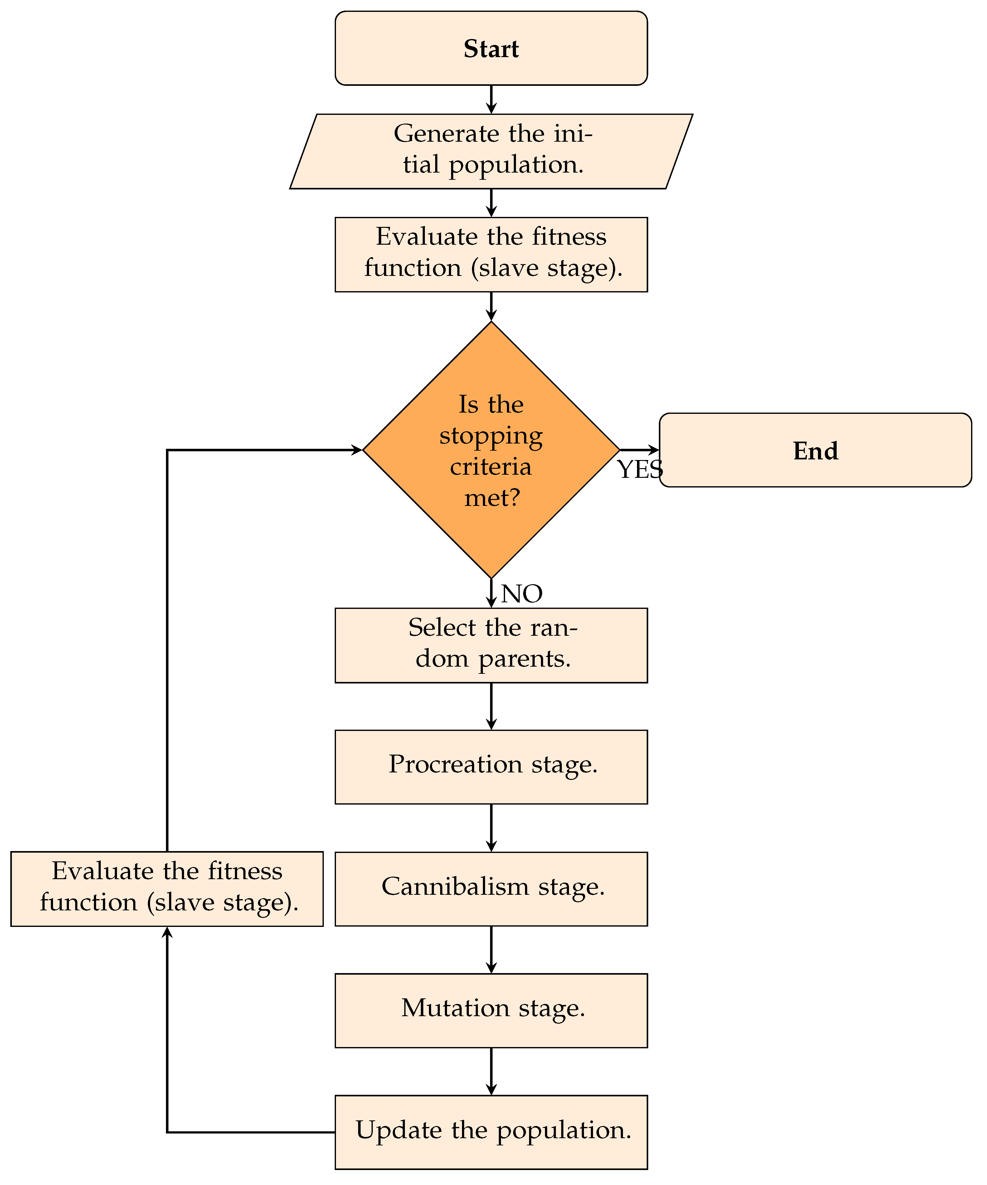
The main characteristics of the BWO are presented in Figure 1.

Each of the main evolution aspects of the BWO depicted in Figure 1 is presented below.

3.1.1. Initial Population

As is typical in combinatorial optimization algorithms, the BWO explores and exploits the solution space by using a set of potential solutions known as the initial population [36]. An individual in the initial population takes the following form:

$$\begin{array}{c}\hfill x_i^t=\left[\begin{array}{c}10,25,\cdots ,k|1.2570,0.1985,\cdots ,q_k^{\mathrm{comp}}\end{array}\right],i=1,2,...,N_s\end{array}$$

(10)

where $x_i^t$ is the ith potential solution (ith spider) at iteration t, and $N_s$ is the number of spiders in the initial population, i.e., the number of candidate solutions. Note that the generation of the initial population is a random process, where the structure of each potential solution in (10) was generated with a uniform distribution [37].

Remark 3.

Each of the potential solution candidates defined by (10) is reviewed to ensure that the first $N_A^{\mathrm{comp}}$ positions are integer numbers between 2 and the number of nodes of the network (i.e., n, which denotes the cardinality of the set $\mathcal{N}$). In addition, the remaining positions between $Q_{min}^{\mathrm{comp}}$ and $Q_{min}^{\mathrm{comp}}$ are selected, using a uniform distribution with real numbers.

It is important to note that the codification employed in this research is discrete-continuous, as the BWO generates the set of nodes where the FACTS must be installed with their corresponding expected sizes [25].

3.1.2. Procreation Stage

This stage of the BWO emulates the generation of multiple solution individuals, i.e., new spiders descending from the initial parents [35]. In the wild, each mating produces about 1000 eggs, out of which only the strongest spiders survive. The general procreation rule in the BWO is defined in (11).

$$\left\{\begin{array}{c}{y}_i^t=\alpha \times x_i^t+(1-\alpha )\times x_j^t\\ y_j^t=\alpha \times x_j^t+(1-\alpha )\times x_i^t\end{array}\right.$$

(11)

where $y_i^t$ and $y_j^t$ are two spiderlings obtained after the union of the two parents $x_i^t$ and $x_j^t$ in the procreation stage. Note that the parents i and j must be different, and $\alpha$ is a vector with values between 0 and 1 and a uniform distribution, which can be associated with the percentage of importance of each parent’s position in the generation of new spiderlings.

Remark 4.

The number of spiderlings generated with rule (11) is defined in the parametrization of the BWO algorithm. In addition, each $y_i^t$ and $y_i^t$ must be checked to ensure that its structure fulfills the conditions assigned in (10). This stage is crucial because it allows keeping all potential solutions feasible in the master optimization stage.

3.1.3. Cannibalism Stage

One of the main characteristics of black widow spiders is their cannibalistic nature, where only strong individuals survive [34]. In this stage, three different cannibalistic behaviors must be analyzed.

i.

Sexual cannibalism, where the females devour the males during or after the procreation stage.

ii.

Spiderlings eating each other: in the BWO, this behavior is established using the cannibalism index ($C_R$), which specifies the number of survivors, i.e., the best solutions after evaluation in the slave stage [28].

iii.

The possibility that the parents are devoured by their offspring. The BWO evaluates the possibility of replacing the parents in the current population with the best spiderlings.

3.1.4. Mutation Stage

In this stage, some of the spiderlings will evidence some distinctive characteristics regarding the parents, which correspond to the mutations occurring in the natural evolution of species within their living communities. The mutation procedure is illustrated in Equation (12).

$$\begin{array}{c}[10,25,\dots ,k | 1.2570,0.1985,\dots ,q_k^{\mathrm{comp}}]\\ \downarrow \\ [k,25,\dots ,10 | 1.2570,0.1985,\dots ,q_k^{\mathrm{comp}}],\end{array}$$

(12)

Remark 5.

Note that, in order to evaluate the feasibility of the spiderlings in the mutation stage, the rotation of the gens in the solution vector must be applied, preserving the exact nature of the decision variables, i.e., only between nodes or only between FACTS sizes.

3.1.5. Stopping Criteria

The exploration and exploitation of the solution space with the BWO ends as follows:

i.

When the maximum number of iterations $t_{max}$ is reached.

ii.

If, after $k_{max}$ iterations, the objective function does not exhibit any improvement (local stopping criteria).

iii.

When the desired convergence is reached.

For more details regarding the implementation of the BWO approach, the reader should consult the references [29,38]

3.2. Slave Stage: Successive Approximation Power Flow Method

As observed in the BWO algorithm depicted in Figure 1, the evolution of the initial population through the solution space, as well as the application of the cannibalism and mutation stages, requires the evaluation of the potential solutions by the slave stage [36]. In this optimization model (1)–(8), the slave stage is used to evaluate each potential FACTS location and size in the power balance constraints (4) and (5). To solve these equations, a numerical method must be used in order to find a solution with adequate convergence [39].

This research adopts the SAPF method to solve the power flow problem in electrical distribution networks due to its easy implementation and efficient convergence [40]. The general SAPF formula is defined in Equation (13).

$$\begin{array}{c}\hfill {\mathbb{V}}_{dh}^{m+1}=-{\mathbf{Y}}_{dd}^{-1}\left({\mathbf{diag}}^{-1}\left({\mathbb{V}}_{dh}^{m,🟉}\right)\left({\mathbb{S}}_{dh}^{🟉}-{\mathbb{S}}_{\mathrm{comp}}^{🟉}\right)+{\mathbf{Y}}_{dg}{\mathbb{V}}_{gh}\right),\left\{\forall h\in \mathcal{H}\right\}\end{array}$$

(13)

where m is the iteration counter; ${\mathbb{V}}_{dh}$ is a complex vector containing the voltage variables in all the demand nodes per period; ${\mathbb{V}}_{gh}$ corresponds to a vector that contains the voltage values in the slack source; ${\mathbf{Y}}_{dd}$ is a square matrix associated with the admittance relations between demand nodes; ${\mathbf{Y}}_{dg}$ is a rectangular matrix that contains the complex relations between the demand and slack nodes; ${\mathbb{S}}_{dh}$ is a vector containing the set of constant demand power loads per node and period; and ${\mathbb{S}}_{\mathrm{comp}}$ corresponds to the vector of complex power injections at the nodes where the FACTS must be placed. Note that ${\mathbb{X}}^{🟉}$ denotes the application of the conjugate operator to the complex vector $\mathbb{X}$.

Remark 6.

Note that the vector ${\mathbb{S}}_{\mathrm{comp}}$ contains the variables that relate the master stage to the slave stage, as the former defines the set of nodes and FACTS sizes. This is fixed in the slave stage to solve the power flow problem with the recursive Formula (13).

The convergence criterion applied to the power flow formula in (13), as recommended by the authors of [40], is the error between two consecutive voltage iterations, i.e.,

$$\begin{array}{c}\hfill \underset{h\in \mathcal{H}}{max}\left\{||{\mathbb{V}}_{dh}^{m+1}|-|{\mathbb{V}}_{dh}^m||\right\}\le \epsilon ,\end{array}$$

(14)

where ${\mathbb{V}}_{dh}^0$ corresponds to the vector with the initial voltage values, which are set as equal to the voltage at the substation bus (i.e., ${\mathbb{V}}_{gh}$). In addition, $\epsilon$ is the maximum tolerance error, set as $1\times {10}^{-10}$ [40].

Once power flow Formula (13) has reached the desired convergence in (14), the expected grid power losses can be calculated:

$$\begin{array}{c}\hfill z_1=C_{kWh}T\sum _{h\in \mathcal{H}}{\mathbb{V}}_h^{\top }\left({\mathbf{Y}}^{🟉}{\mathbb{V}}_h\right){\mathsf{\Delta }}_h,\end{array}$$

(15)

where ${\mathbb{V}}_h$ is the vector containing the voltage profiles in the distribution network, including the slack source per period, i.e., ${\mathbb{V}}_h={\left[{\mathbb{V}}_{gh}{\mathbb{V}}_{dh}\right]}^{\top }$, and $\mathbf{Y}$ is the nodal admittance matrix of the distribution network under analysis.

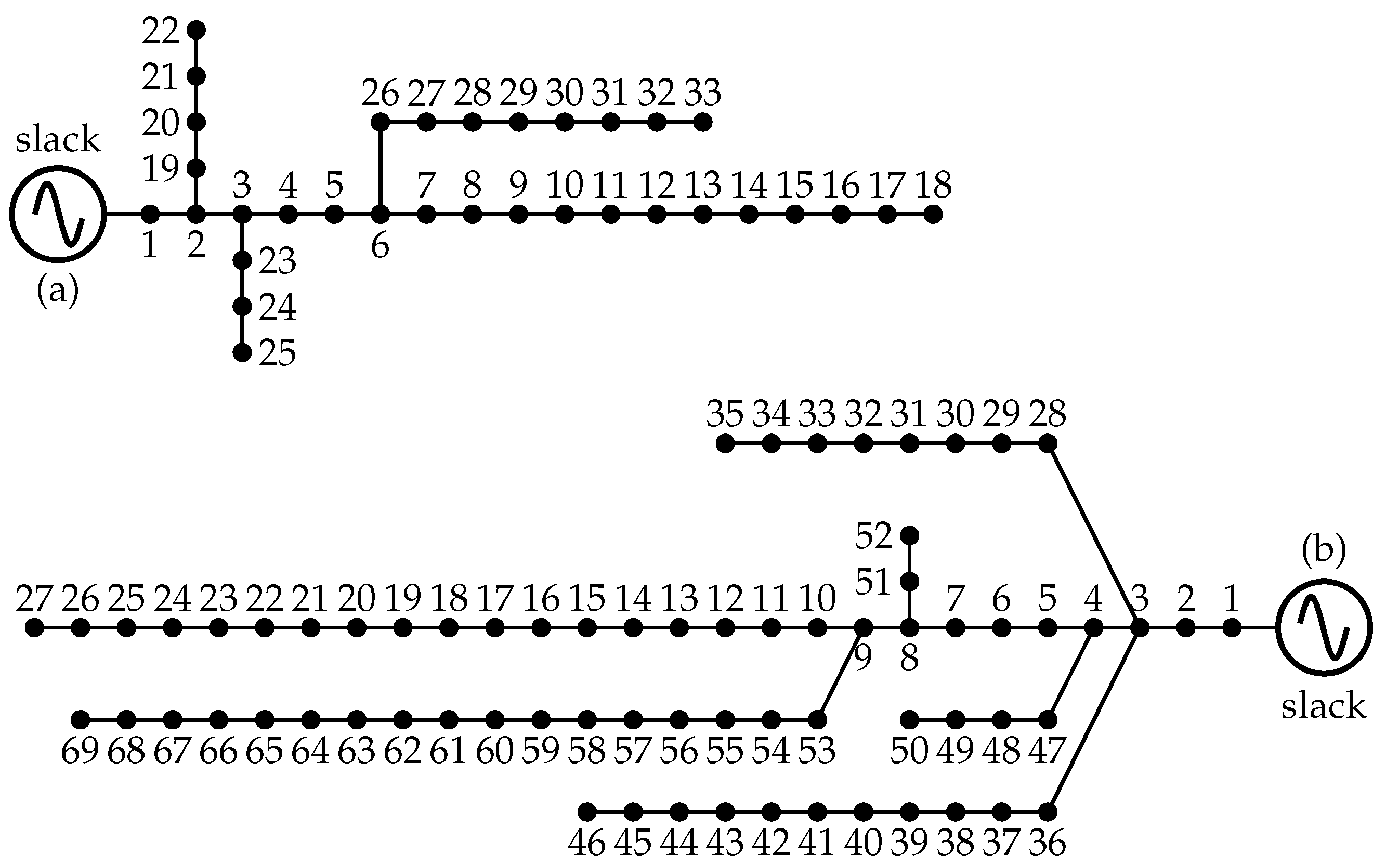
4. Test Feeder Characterization

To validate the proposed optimization methodology for locating and sizing FACTS in electrical distribution networks, the IEEE 33- and 69-bus grids with radial configurations are considered as test feeders. The electrical configuration of both distribution networks is depicted in Figure 2. In addition, their electrical parametrization regarding impedances and peak load consumptions are listed in

Table 2. IEEE 33-bus system parameters.

Node i	Node j	${\mathit{R}}_{\mathit{ij}}$ ($\mathbf{\Omega }$)	${\mathit{X}}_{\mathit{ij}}$ ($\mathbf{\Omega }$)	${\mathit{P}}_{\mathit{j}}$ (kW)	${\mathit{Q}}_{\mathit{j}}$ (kvar)	Node i	Node j	${\mathit{R}}_{\mathit{ij}}$ ($\mathbf{\Omega }$)	${\mathit{X}}_{\mathit{ij}}$ ($\mathbf{\Omega }$)	${\mathit{P}}_{\mathit{j}}$ (kW)	${\mathit{Q}}_{\mathit{j}}$ (kvar)
1	2	0.0922	0.0477	100	60	17	18	0.7320	0.5740	90	40
2	3	0.4930	0.2511	90	40	2	19	0.1640	0.1565	90	40
3	4	0.3660	0.1864	120	80	19	20	1.5042	1.3554	90	40
4	5	0.3811	0.1941	60	30	20	21	0.4095	0.4784	90	40
5	6	0.8190	0.7070	60	20	21	22	0.7089	0.9373	90	40
6	7	0.1872	0.6188	200	100	3	23	0.4512	0.3083	90	50
7	8	1.7114	1.2351	200	100	23	24	0.8980	0.7091	420	200
8	9	1.0300	0.7400	60	20	24	25	0.8960	0.7011	420	200
9	10	1.0400	0.7400	60	20	6	26	0.2030	0.1034	60	25
10	11	0.1966	0.0650	45	30	26	27	0.2842	0.1447	60	25
11	12	0.3744	0.1238	60	35	27	28	1.0590	0.9337	60	20
12	13	1.4680	1.1550	60	35	28	29	0.8042	0.7006	120	70
13	14	0.5416	0.7129	120	80	29	30	0.5075	0.2585	200	600
14	15	0.5910	0.5260	60	10	30	31	0.9744	0.9630	150	70
15	16	0.7463	0.5450	60	20	31	32	0.3105	0.3619	210	100
16	17	1.2860	1.7210	60	20	32	33	0.3410	0.5302	60	40

and

Table 3. IEEE 69-bus system parameters.

Node i	Node j	${\mathit{R}}_{\mathit{ij}}$ ($\mathbf{\Omega }$)	${\mathit{X}}_{\mathit{ij}}$ ($\mathbf{\Omega }$)	${\mathit{P}}_{\mathit{j}}$ (kW)	${\mathit{Q}}_{\mathit{j}}$ (kvar)	Node i	Node j	${\mathit{R}}_{\mathit{ij}}$ ($\mathbf{\Omega }$)	${\mathit{X}}_{\mathit{ij}}$ ($\mathbf{\Omega }$)	${\mathit{P}}_{\mathit{j}}$ (kW)	${\mathit{Q}}_{\mathit{j}}$ (kvar)
1	2	0.0005	000012	0.00	0.00	3	36	0.0044	0,0108	26.00	18.55
2	3	0.0005	0.0012	0.00	0.00	36	37	0.0640	0.1565	26.00	18.55
3	4	0.0015	0.0036	0.00	0.00	37	38	0.1053	0.1230	0.00	0.00
4	5	0.0251	0.0294	0.00	0.00	38	39	0.0304	0.0355	24.00	17.00
5	6	0.3660	0.1864	2.60	2.20	39	40	0.0018	0.0021	24.00	17.00
6	7	0.3810	0.1941	40.40	30.00	40	41	0.7283	0.8509	1.20	1.00
7	8	0.0922	0.0470	75.00	54.00	41	42	0.3100	0.3623	0.00	0.00
8	9	0.0493	0.0251	30.00	22.00	42	43	0.0410	0.0478	6.00	4.30
9	10	0.8190	0.2707	28.00	19.00	43	44	0.0092	0.0116	0.00	0.00
10	11	0.1872	0.0619	145.00	104.00	44	45	0.1089	0.1373	39.22	26.30
11	12	0.7114	0.2351	145.00	104.00	45	46	0.0009	0.0012	29.22	26.30
12	13	1.0300	0.3400	8.00	5.00	4	47	0.0034	0.0084	0.00	0.00
13	14	1.0440	0.3450	8.00	5.50	47	48	0.0851	0.2083	79.00	56.40
14	15	1.0580	0.3496	0.00	0.00	48	49	0.2898	0.7091	384.70	274.50
15	16	0.1966	0.0650	45.50	30.00	49	50	0.0822	0.2011	384.70	274.50
16	17	0.3744	0.1238	60.00	35.00	8	51	0.0928	0.0473	40.50	28.30
17	18	0.0047	0.0016	60.00	35.00	51	52	0.3319	0.1114	3.60	2.70
18	19	0.3276	0.1083	0.00	0.00	9	53	0.1740	0.0886	4.35	3.50
19	20	0.2106	0.0690	1.00	0.60	53	54	0.2030	0.1034	26.40	19.00
20	21	0.3416	0.1129	114.00	81.00	54	55	0.2842	0.1447	24.00	17.20
21	22	0.0140	0.0046	5.00	3.50	55	56	0.2813	0.1433	0.00	0.00
22	23	0.1591	0.0526	0.00	0.00	56	57	1.5900	0.5337	0.00	0.00
23	24	0.3463	0.1145	28.00	20.00	57	58	0.7837	0.2630	0.00	0.00
24	25	0.7488	0.2475	0.00	0.00	58	59	0.3042	0.1006	100.00	72.00
25	26	0.3089	0.1021	14.00	10.00	59	60	0.3861	0.1172	0.00	0.00
26	27	0.1732	0.0572	14.00	10.00	60	61	0.5075	0.2585	1244.00	888.00
3	28	0.0044	0.0108	26.00	18.60	61	62	0.0974	0.0496	32.00	23.00
28	29	0.0640	0.1565	26.00	18.60	62	63	0.1450	0.0738	0.00	0.00
29	30	0.3978	0.1315	0.00	0.00	63	64	0.7105	0.3619	227.00	162.00
30	31	0.0702	0.0232	0.00	0.00	64	65	1.0410	0.5302	59.00	42.00
31	32	0.3510	0.1160	0.00	0.00	11	66	0.2012	0.0611	18.00	13.00
32	33	0.8390	0.2816	14.00	10.00	66	67	0.0470	0.0140	18.00	13.00
33	34	1.7080	0.5646	19.50	14.00	12	68	0.7394	0.2444	28.00	20.00
34	35	1.4740	0.4873	6.00	4.00	68	69	0.0047	0.0016	28.00	20.00

, respectively.

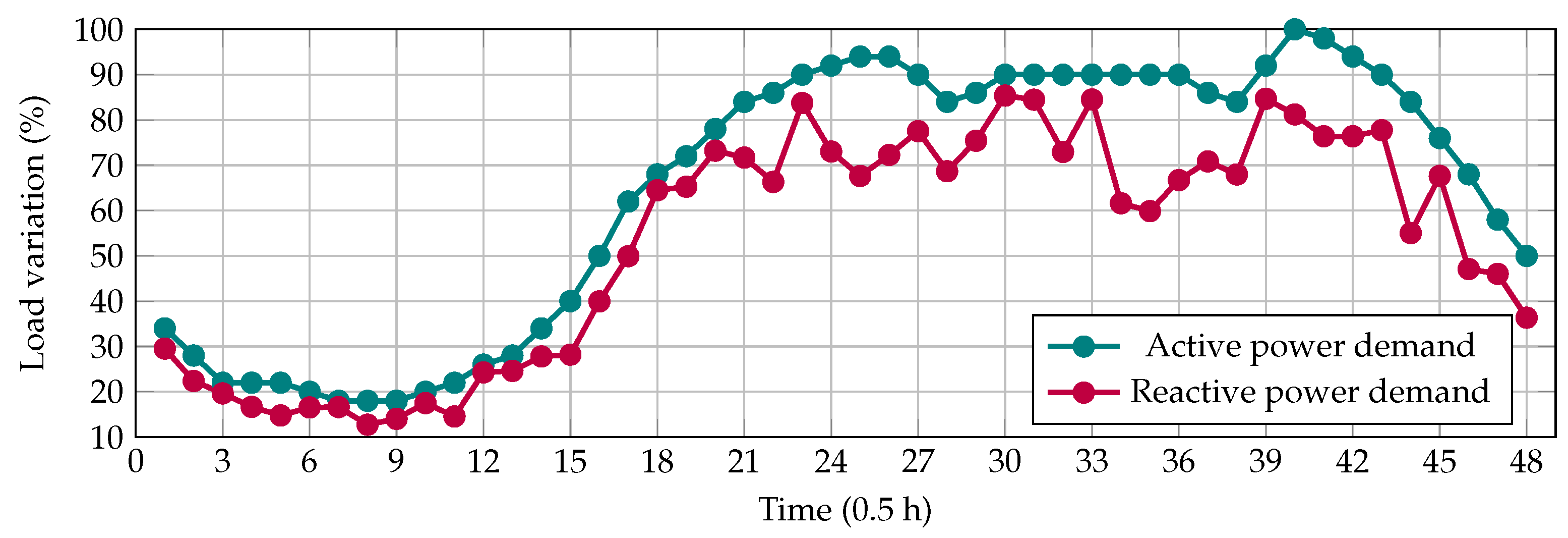
To illustrate the effect of the daily active and reactive power profiles on the expected annual grid operating costs, i.e., the costs of the energy losses defined by $z_1$ in (1), the active and reactive power curves considered in the simulation scenarios are depicted in Figure 3.

To evaluate the objective function, each component must be parameterized (i.e., $z_1$ and $z_2$) in Equations (1) and (2). The parameters of these equations are listed in

Table 4. Parametrization of the objective function considering different FACTS devices.

Par.	Value	Unit	Par.	Value	Unit
$C_{\mathrm{kWh}}$	0.1390	USD/kWh	T	365	Days
${\mathsf{\Delta }}_h$	0.50	h	$k_1$	6/2190	1/Days
$k_2$	10	Years	—	—	—
FACTS parameters
Device	${\mathbf{\omega }}_{\mathbf{1}}$(USD/Mvar3)		${\mathbf{\omega }}_{\mathbf{2}}$(USD/Mvar2)		${\mathbf{\omega }}_{\mathbf{1}}$(USD/Mvar)
SVC	0.30		−305.10		127,380
TCSC	1.50		−713.00		153,750
UPFC	0.30		−269.10		188,220

. Note that the costs of the FACTS were adapted from [28].

5. Numerical Results

For the computational implementation of the proposed master–slave strategy, MATLAB software, Mathworks, Natick, Massachusetts, USA (version $2021b$) was employed on a PC with an AMD Ryzen 7 3700 $2.3$ GHz processor and 16.0 GB RAM, running a 64-bit version of Microsoft Windows 10 Single Language. The BWO and the successive approximations power flow method were implemented with our own scripts. The parametrization of the BWO includes 100 repetitions, 10 individuals in the population, and 1000 iterations.

The following simulation scenarios were considered to validate the effectiveness of our approach to locating and sizing FACTS in electrical distribution networks.

i.

C1: The validation of the proposed optimization approach with respect to the literature reports in the case of the IEEE 33- and 69-bus grids regarding the installation of SVCs, which the authors of [25] have denoted as D-STATCOMs. For comparison purposes, this research uses the vortex search algorithm (VSA), the hybrid genetic algorithm with the particle swarm optimizer (GA/PSO), and the solution of the exact MINLP model in GAMS. In order to make fair comparisons, all the listed combinatorial optimizers were set with the same population sizes, number of iterations, and stopping criteria.

ii.

C2: The evaluation of the proposed optimization approach, considering all three FACTS analyzed (i.e., VSC, UPFC, and TCSC devices) in the IEEE 33-, 69, and 85-bus grids.

Regarding the optimization algorithms used for comparison, it is essential to mention the following.

i.

The VSA is a combinatorial method from the family of physics-inspired optimizers that models the behavior of fluids being shaken in pipes [41]. This behavior is modeled through Gaussian distributions that allow exploring and exploiting the solution space in optimization problems, starting with the highest possible hyper-ellipse that covers the entire multi-dimensional space, where the hyper-center represents the best current solution [42]. The main idea is that all solutions are uniformly distributed in this hyper-ellipse with a Gaussian distribution. Then, during the exploration process, the radius of the hyper-ellipse is continuously reduced via Gamma functions, which allows starting to exploit the solution space in the most promising region of solutions [43].

ii.

The GA/PSO approach is a combination of the classical genetic algorithm (GA) with the particle swarm optimizer (PSO) in a master–slave connection, where the GA is used to define the set of nodes where the FACTS must be installed (using discrete codification). In contrast, the PSO approach is entrusted with exploring the solution space to define the best FACTS sizes [25]. The main characteristic of this master–slave optimizer is the use of two nature-inspired algorithms to address complex combinatorial optimization problems, where the GA is selected due to its excellent performance for discrete variables [44], and the PSO is chosen based on its effectiveness in dealing with continuous variables [45].

iii.

The exact MINLP solvers in GAMS (i.e., the COUENNE and the BONMIN solvers) are optimization tools that deal with MINLP models by using a combination of interior-point methods and branch-and-cut algorithms to explore and exploit the solution space [46]. The main advantage of using the GAMS software for solving MINLP models is that the researcher focuses their attention on the mathematical modeling and the accuracy in representing the real analyzed phenomena with equations, not on the solution technique itself [47].

5.1. Comparative Analysis with Literature Reports

Table 5. Numerical results in the IEEE 33- and 69- grids when compared to the proposed BWO approach and the literature reports.

IEEE 33-Bus Grid
Method	Location	Size (Mvar)	${\mathbf{z}}_{\mathbf{cost}}$(USD/Year)	Reduction (%)	Time (s)
Benchmark case	—	—	112,740.90	—	—
COUENNE	$\left[\begin{array}{c}16,17,18\end{array}\right]$	$\left[\begin{array}{c}0.0109,0.0224,0.2065\end{array}\right]$	107,589.50	4.56	3.03
BONMIN	$\left[\begin{array}{c}17,18,30\end{array}\right]$	$\left[\begin{array}{c}0.0339,0.0227,0.2395\end{array}\right]$	102,447.29	9.13	7.59
GA/PSO	$\left[\begin{array}{c}14,30,31\end{array}\right]$	$\left[\begin{array}{c}0.1599,0.3497,0.1117\end{array}\right]$	98,511.63	12.62	6417.91
VSA	$\left[\begin{array}{c}14,30,32\end{array}\right]$	$\left[\begin{array}{c}0.1599,0.3591,0.1072\end{array}\right]$	98,497.90	12.63	59.64
BWO	$\left[\begin{array}{c}14,30,32\end{array}\right]$	$\left[\begin{array}{c}0.1599,0.3591,0.1072\end{array}\right]$	98,497.90	12.63	44.08
IEEE 69-Bus Grid
Method	Location	Size (Mvar)	${\mathbf{z}}_{\mathbf{cost}}$(USD/Year)	Reduction (%)	Time (s)
Benchmark case	—	—	119,715.63	—	—
GA/PSO	$\left[\begin{array}{c}21,61,64\end{array}\right]$	$\left[\begin{array}{c}0.0839,0.4600,0.1139\end{array}\right]$	102,990.79	13.97	9325.89
VSA	$\left[\begin{array}{c}21,61,64\end{array}\right]$	$\left[\begin{array}{c}0.0839,0.4601,0.1139\end{array}\right]$	102,990.79	13.97	202.66
BWO	$\left[\begin{array}{c}21,61,64\end{array}\right]$	$\left[\begin{array}{c}0.0839,0.4601,0.1139\end{array}\right]$	102,990.79	13.97	176.74

presents the numerical results obtained when D-STATCOMs (SVCs) are installed in the IEEE 33- and 69-bus grids.

The numerical results in Table 5 show the following:

i.

The VSA and the proposed BWO approach find the same optimal objective function value for both test feeders, corresponding to reductions of about $12.63\%$ and $13.97\%$ for the test feeders, respectively. However, the main advantage of the proposed BWO approach is that it requires a lower processing time to solve the problem regarding the optimal location of D-STATCOMs in both test feeders, with values of about 44.08 s and 176.74 s, respectively.

ii.

The combination of the GA and PSO algorithms exhibited an adequate performance in both test feeders, reaching the exact solution of the BWO approach in the case of the IEEE 69-bus grid, as well as a near-optimal solution for the IEEE 33-bus grid. However, the main complication of this approach lies in its required processing times, which are higher than 6400 s in both simulation scenarios. This behavior is expected given that the GA approach defines the nodes where the D-STATCOMs must be located. In addition, the PSO approach is entrusted with solving the optimal reactive power flow problem to determine their optimal sizes. This implies that there are two combinatorial optimization methods working under a master–slave connection, thus increasing the total processing times required to solve the studied problem.

iii.

The exact solution of the MINLP model with BONMIN and COUENNE showed these to be stuck in locally optimal solutions in the case of the IEEE 33-bus grid, and they did not reach a possible solution point for the IEEE 69-bus grid. This behavior shows the high complexity of the model that represents the problem under study, which is due to its nonlinearities and non-convexities, thus confirming the need for efficient master–slave optimizers, such as the proposed BWO approach.

5.2. Location and Sizing of FACTS in the IEEE 33- and 69-Bus Grids

This section presents the general objective function behavior and the nodes and sizes of the different FACTS analyzed when implementing the BWO approach.

Table 6. Results in the IEEE 33- and 69-bus grids regarding the integration of FACTS with the proposed BWO approach.

IEEE 33-Bus Grid
FACTS Devices	Location	Size (Mvar)	${\mathbf{z}}_{\mathbf{cost}}$(USD/Year)	Reduction (%)	Time (s)
Benchmark case	—	—	112,740.90	—	—
UPFC	$\left[\begin{array}{c}14,30,32\end{array}\right]$	$\left[\begin{array}{c}0.1340,0.2980,0.1074\end{array}\right]$	102,043.23	9.49	43.94
TCSC	$\left[\begin{array}{c}14,30,32\end{array}\right]$	$\left[\begin{array}{c}0.1486,0.3337,0.1064\end{array}\right]$	100,093.29	11.22	43.97
SVC	$\left[\begin{array}{c}14,30,32\end{array}\right]$	$\left[\begin{array}{c}0.1599,0.3591,0.1072\end{array}\right]$	98,497.90	12.63	44.08
IEEE 69-Bus Grid
FACTS Device	Location	Size (Mvar)	${\mathbf{z}}_{\mathbf{cost}}$(USD/Year)	Reduction (%)	Time (s)
Benchmark case	—	—	119,715.63	—	—
UPFC	$\left[\begin{array}{c}21,61,64\end{array}\right]$	$\left[\begin{array}{c}0.0397,0.4008,0.1142\end{array}\right]$	106,679.88	10.89	177.72
TCSC	$\left[\begin{array}{c}21,61,64\end{array}\right]$	$\left[\begin{array}{c}0.0647,0.4363,0.1125\end{array}\right]$	104,658.03	12.58	173.12
SVC	$\left[\begin{array}{c}21,61,64\end{array}\right]$	$\left[\begin{array}{c}0.0839,0.4601,0.1139\end{array}\right]$	102,990.79	13.97	176.74

presents the best numerical solutions with the proposed BWO approach in both test feeders.

The numerical results in Table 6 show the following:

i.

In the IEEE 33-bus grid, the selected nodes for installing FACTS are 14, 30, and 32, with node 30 being the most sensitive regarding reactive power injection, given that this node was assigned the largest FACTS size. In addition, the most efficient FACTS element regarding the final objective function value corresponds to SVCs, with a reduction of about 12.63% in the expected annual operating costs, followed by TCSCs with a reduction of about 11.22% concerning the benchmark case.

ii.

In the IEEE 69-bus grid, the BWO approach identifies nodes 21, 61, and 64 as the most effective for optimal reactive power compensation, where node 61 is the most sensitive to locate and size compensation devices, with values larger than 400 kvar for all the FACTS analyzed. As with the IEEE 33-bus grid, the most effective device for the reduction in the objective function value corresponds to SVCs, which allow reaching a reduction of about 13.97%, followed by the TCSCs with a reduction of about 12.58%

It is worth mentioning that the main result in Table 6 is that, regardless of the FACTS analyzed, the BWO approach identifies the same set of nodes for the IEEE 33- and 69-bus grids. This can be attributed to the fact that (2) is a cubic function with the same numerical structure as that seen in Table 4, i.e., the same signs for the $\omega$ coefficients. In addition, the variations in the final objective functions, as expected, are associated with the $\omega$ coefficients in this objective function; the FACTS device with the most expensive linear costs (i.e., the value of ${\omega }_3$) reaches the lowest reduction in the annual grid operating costs. In this sense, the expected reductions regarding the general objective function are highly dependent on the linear coefficient. In this regard, note that, in Table 6, these reductions are ordered increasingly by the integration of the UPFC, the TCSC, and the SVC.

Finally, with respect to the processing times spent in locating the FACTS in the IEEE 33- and 69-bus grids, Table 6 shows that less than 45 s and 177 s are required to deal with the efficient integration of reactive power compensators in both test feeders, respectively. These processing times can be considered to be very fast, taking into account that the dimensions of the solution spaces in both systems imply 4960 and 50,116 possible nodal combinations for locating SVCs, UPFCs, and TCSCs, with the main issue that, for each possible combination, the solution space of the nonlinear programming component of the analyzed optimization model is infinite. This behavior regarding processing times confirms the BWO method’s efficiency in solving the optimal reactive power compensation problem in distribution grids.

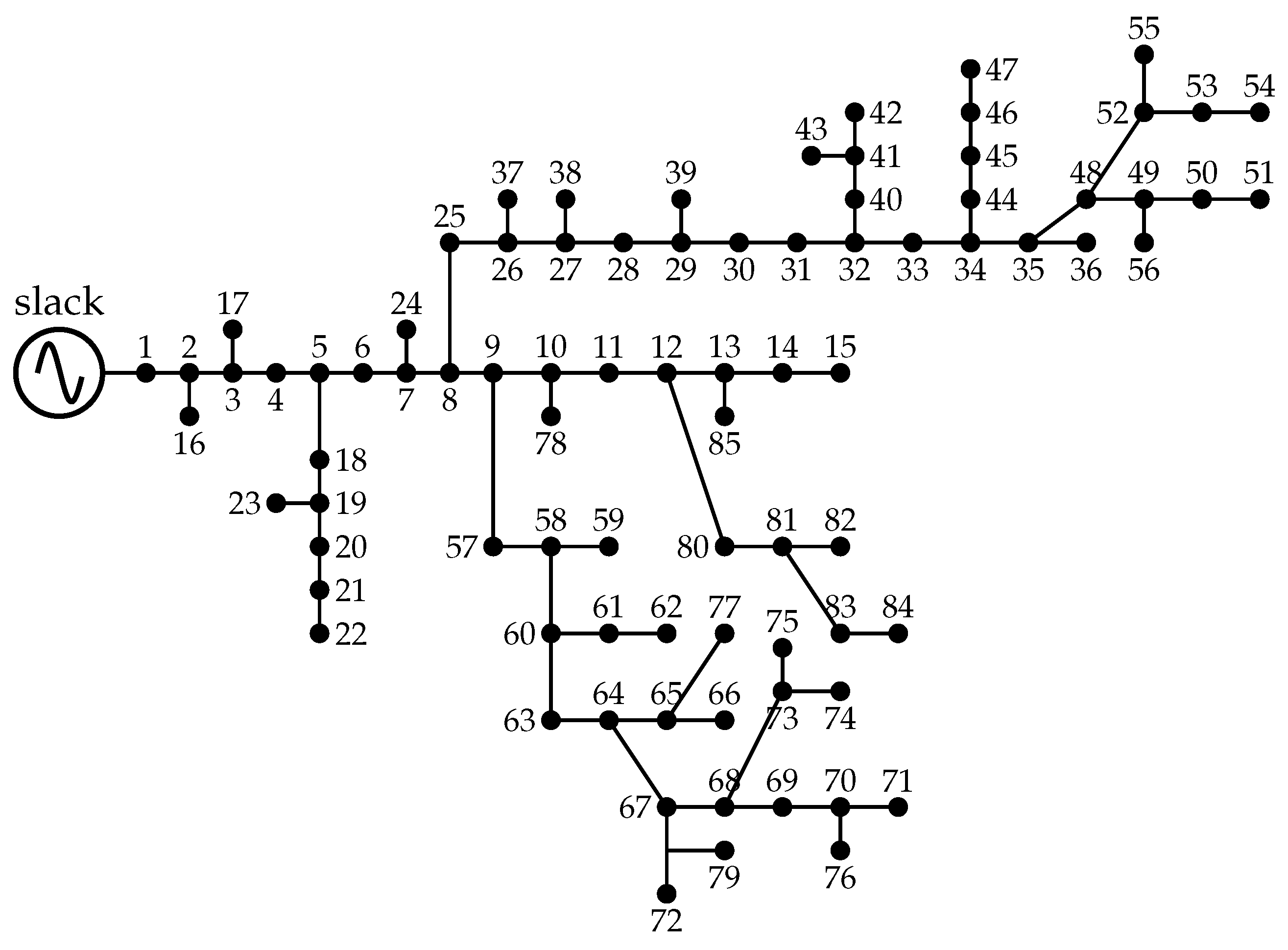
5.3. Evaluating the Scalability of the Proposed Master–Slave Methodology

The IEEE 85-bus grid was used as a test feeder to demonstrate the proposed optimization methodology’s effectiveness and robustness. This is a medium-voltage distribution network operated with 11 kV at the substation bus. The electrical configuration and all electrical parameters of this test feeder are presented in Figure 4 and

Table 7. Electrical data on the IEEE 85-bus network.

k	m	${\mathit{R}}_{\mathit{km}}$ ($\mathbf{\Omega }$)	${\mathit{x}}_{\mathit{km}}$ ($\mathbf{\Omega }$)	${\mathit{P}}_{\mathit{k}}$ (kW)	${\mathit{Q}}_{\mathit{k}}$ (kW)	k	m	${\mathit{R}}_{\mathit{km}}$ ($\mathbf{\Omega }$)	${\mathit{x}}_{\mathit{km}}$ ($\mathbf{\Omega }$)	${\mathit{P}}_{\mathit{k}}$ (kW)	${\mathit{Q}}_{\mathit{k}}$ (kW)
1	2	0.108	0.075	0	0	34	44	1.002	0.416	35.28	35.99
2	3	0.163	0.112	0	0	44	45	0.911	0.378	35.28	35.99
3	4	0.217	0.149	56	57.13	45	46	0.911	0.378	35.28	35.99
4	5	0.108	0.074	0	0	46	47	0.546	0.226	14	14.28
5	6	0.435	0.298	35.28	35.99	35	48	0.637	0.264	0	0
6	7	0.272	0.186	0	0	48	49	0.182	0.075	0	0
7	8	1.197	0.820	35.28	35.99	49	50	0.364	0.151	36.28	37.01
8	9	0.108	0.074	0	0	50	51	0.455	0.189	56	57.13
9	10	0.598	0.410	0	0	48	52	1.366	0.567	0	0
10	11	0.544	0.373	56	57.13	52	53	0.455	0.189	35.28	35.99
11	12	0.544	0.373	0	0	53	54	0.546	0.226	56	57.13
12	13	0.598	0.410	0	0	52	55	0.546	0.226	56	57.13
13	14	0.272	0.186	35.28	35.99	49	56	0.546	0.226	14	14.28
14	15	0.326	0.223	35.28	35.99	9	57	0.273	0.113	56	57.13
2	16	0.728	0.302	35.28	35.99	57	58	0.819	0.340	0	0
3	17	0.455	0.189	112	114.26	58	59	0.182	0.075	56	57.13
5	18	0.820	0.340	56	57.13	58	60	0.546	0.226	56	57.13
18	19	0.637	0.264	56	57.13	60	61	0.728	0.302	56	57.13
19	20	0.455	0.189	35.28	35.99	61	62	1.002	0.415	56	57.13
20	21	0.819	0.340	35.28	35.99	60	63	0.182	0.075	14	14.28
21	22	1.548	0.642	35.28	35.99	63	64	0.728	0.302	0	0
19	23	0.182	0.075	56	57.13	64	65	0.182	0.075	0	0
7	24	0.910	0.378	35.28	35.99	65	66	0.182	0.075	56	57.13
8	25	0.455	0.189	35.28	35.99	64	67	0.455	0.189	0	0
25	26	0.364	0.151	56	57.13	67	68	0.910	0.378	0	0
26	27	0.546	0.226	0	0	68	69	1.092	0.453	56	57.13
27	28	0.273	0.113	56	57.13	69	70	0.455	0.189	0	0
28	29	0.546	0.226	0	0	70	71	0.546	0.226	35.28	35.99
29	30	0.546	0.226	35.28	35.99	67	72	0.182	0.075	56	57.13
30	31	0.273	0.113	35.28	35.99	68	73	1.184	0.491	0	0
31	32	0.182	0.075	0	0	73	74	0.273	0.113	56	57.13
32	33	0.182	0.075	14	14.28	73	75	1.002	0.416	35.28	35.99
33	34	0.819	0.340	0	0	70	76	0.546	0.226	56	57.13
34	35	0.637	0.264	0	0	65	77	0.091	0.037	14	14.28
35	36	0.182	0.075	35.28	35.99	10	78	0.637	0.264	56	57.13
26	37	0.364	0.151	56	57.13	67	79	0.546	0.226	35.28	35.99
27	38	1.002	0.416	56	57.13	12	80	0.728	0.302	56	57.13
29	39	0.546	0.226	56	57.13	80	81	0.364	0.151	0	0
32	40	0.455	0.189	35.28	35.99	81	82	0.091	0.037	56	57.13
40	41	1.002	0.416	0	0	81	83	1.092	0.453	35.28	35.99
41	42	0.273	0.113	35.28	35.99	83	84	1.002	0.416	14	14.28
41	43	0.455	0.189	35.28	35.99	13	85	0.819	0.340	35.28	35.99

.

Table 8. Location and sizing of FACTS in the IEEE 85-bus grid with the proposed BWO algorithm.

FACTS Devices	Location	Size (Mvar)	${\mathbf{z}}_{\mathbf{cost}}$ (USD/Year)	Reduction (%)	Time (s)
Benchmark case	—	—	154,651.95	—	—
UPFC	$\left[\begin{array}{c}12,34,67\end{array}\right]$	$\left[\begin{array}{c}0.2093,0.3760,0.3069\end{array}\right]$	119,288.35	22.87	265.98
TCSC	$\left[\begin{array}{c}12,34,67\end{array}\right]$	$\left[\begin{array}{c}0.2318,0.3857,0.3195\end{array}\right]$	116,122.78	24.91	255.54
SVC	$\left[\begin{array}{c}12,34,67\end{array}\right]$	$\left[\begin{array}{c}0.2490,0.3930,0.3289\end{array}\right]$	113,619.97	26.53	260.26

presents the numerical validations of the proposed BWO algorithm in the optimal location and sizing of FACTS in the IEEE 85-bus grid.

The numerical results in Table 8 show the following:

i.

The proposed BWO algorithm finds the exact nodal locations for each FACTS device, i.e., nodes 12, 34, and 67. In addition, the maximum reactive power injection per node is observed in the SVC, with values of 249, 393, and 328.9 kvar, respectively.

ii.

The minimization of the annual operating costs varies from USD 35,363.6 (when UPFCs are installed) to USD 41,031.98 (when SVCs are installed). These values imply a difference of about 5668.38 USD per year of operation in favor of the SVC. In addition, the expected annual costs reduction using FACTS in the IEEE 85-bus grid are 22.87, 24.91, and 26.53% when considering UPFCs, TCSCs, and SVCs, respectively.

iii.

Regarding processing times, the proposed BWO approach takes between 255 and 266 s on average to reach an efficient solution to the problem under analysis. These times can be considered to be efficient, in light of the fact that only the size of the discrete component of the optimization model is about 95284 possible options, each with infinite possibilities regarding the expected nominal size of the FACTS.

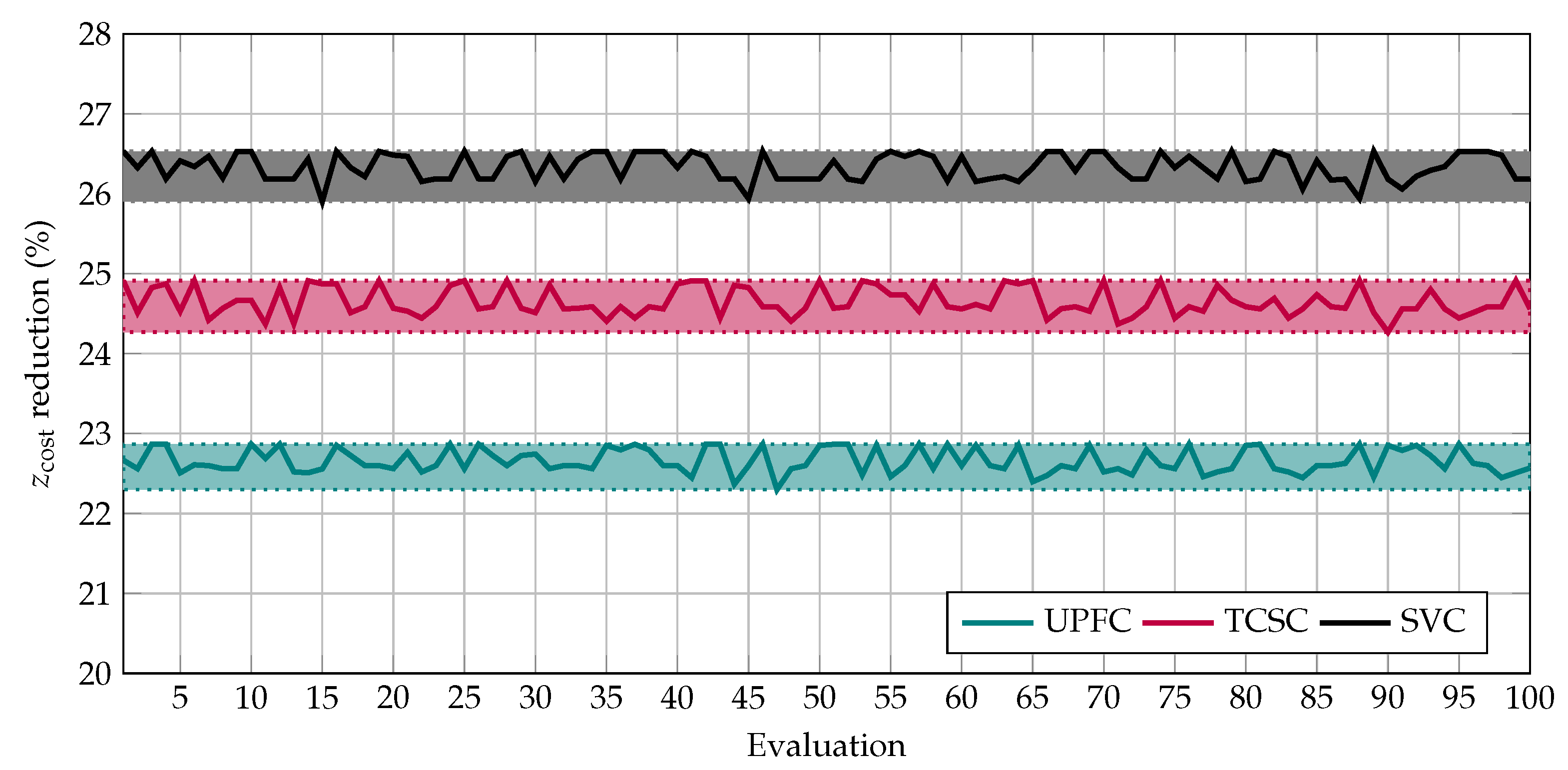
To confirm the effectiveness of the proposed BWO algorithm in siting and locating FACTS, Figure 5 presents the reductions in the objective function value after 100 runs for each compensation device.

Figure 5 shows the variations in the objective function with each compensation system inside a little band. In the case of the UPFC, these variations are between $22.30\%$ and $22.87\%$, i.e., a difference of about $0.57\%$. In the case of the TCSC, these margins are about $24.27\%$ and $24.91\%$, which represents a difference of about $0.64\%$. In contrast, the reduction margins with SVCs are between $25.91\%$ and $26.53\%$, i.e., a difference of about $0.62\%$. Note that the small difference between the best and the worst solution reached with the proposed BWO algorithm per compensation device (lower than 0.64%) confirms that, in each run of the solution methodology, an adequate solution for the studied problem is found, ensuring an excellent annual expected operating costs reduction. This is very attractive for distribution companies, as the BWO algorithm can be considered to be an adequate solution methodology to establish their investment plans regarding reactive power compensation, with different options for locating and sizing FACTS in their grids.

6. Conclusions and Future Work

Via a master–slave methodology, this research analyzed the problem regarding the optimal integration of FACTS in electrical distribution networks in order to minimize the expected annual costs of energy losses, added with the investments in compensation devices. Discrete-continuous codification was employed to represent the set of nodes where the FACTS must be placed and their corresponding size. The exact MINLP model was solved using a decoupling methodology, where the BWO approach defines the location and size of the FACTS, and a power flow solution based on the SAPF approach evaluates the multi-period power flow to determine the expected annual costs of the energy losses.

A comparative analysis with the BONMIN and COUENNE solvers and the VSA and GA/PSO approaches was carried out in two test feeders, considering the existing literature reports with respect to D-STATCOMs (SVCs in this research), which showed that the BWO approach reaches the exact numerical solution found with the VSA in both test feeders, with the main advantage being that the expected processing times are minimal in comparison with the methods used for comparison. On the other hand, the GAMS solvers, due to the complexity of the exact MINLP formulation, converged to locally optimal solutions in the IEEE 33-bus grid and did not provide any feasible solution for the IEEE 69-bus grid. In addition, the GA/PSO approach, even though it efficiently dealt with the solutions of the exact MINLP model in both test feeders, required very long processing times (more than 6400 s), thus affecting the expected trade-off between the objective function value and the computational resources.

The optimal location of the FACTS with the proposed BWO approach, evaluated in the IEEE 33-, 69-, and 85-bus grids, yielded the same set of nodes regardless of the FACTS device analyzed. In the case of the IEEE 33-bus grid, the set of nodes with the best numerical performance included 14, 30, and 32. Node 30 exhibits the most sensitive performance regarding the reactive power required for installation. As for the IEEE 69-bus grid, the set of nodes identified for the optimal location of FACTS included 21, 61, and 64, where node 61 was the most sensitive for installing reactive power compensators. Regarding the IEEE 85-bus grid, the set of nodes identified for the optimal location of FACTS included 12, 34, and 67, where node 34 was the most sensitive.

As for the final objective function value, it was observed that the best FACTS corresponded to SVCs. In the IEEE 33-bus grid, the final reduction obtained by SVCs in the objective function was about $12.63\%$, followed by TCSCs with a value of $11.22\%$. In the case of the IEEE 69-bus grid, these reductions were about $12.58\%$ and $13.97\%$. UPFCs ranked last, with reductions of about 9.49% and 10.89% in the IEEE 33- and 69-bus grids, respectively. For the IEEE 85-bus grid, these reductions were 22.87% with UPFCs, 24.91% using TCSCs, and 26.53% with SVCs.

The processing times required by the proposed BWO for the optimal location of FACTS in the IEEE 33-, 69-, and 85-bus grids (i.e., about 45 s, 177 s, and 266 s, respectively) confirmed the effectiveness of the master–slave approach proposed in this research, considering the infinite dimensions of the solution space for each possible nodal combination.

For future works, the following works can be conducted: (i) the reformulation of the exact MINLP model through a mixed-integer convex formulation to ensure solution uniqueness in each execution, as well as the possibility of finding the best possible solution, i.e., the global optimum, and (ii) the combination of the FACTS analyzed with renewable generation and energy storage systems to reduce the energy purchasing costs in isolated electrical networks fed by diesel sources.

References

- Shahnia, F.; Arefi, A.; Ledwich, G. (Eds.) Electric Distribution Network Planning; Springer: Singapore, 2018. [Google Scholar] [CrossRef]
- Odongo, G.Y.; Musabe, R.; Hanyurwimfura, D.; Bakari, A.D. An Efficient LoRa-Enabled Smart Fault Detection and Monitoring Platform for the Power Distribution System Using Self-Powered IoT Devices. IEEE Access 2022, 10, 73403–73420. [Google Scholar] [CrossRef]
- Lavorato, M.; Franco, J.F.; Rider, M.J.; Romero, R. Imposing Radiality Constraints in Distribution System Optimization Problems. IEEE Trans. Power Syst. 2012, 27, 172–180. [Google Scholar] [CrossRef]
- Farrag, M.A.; Zahra, M.G.; Omran, S. Planning models for optimal routing of radial distribution systems. Int. J. Appl. Power Eng. (IJAPE) 2021, 10, 108. [Google Scholar] [CrossRef]
- Díaz, P. Proposal for Improvements to Reduce Electrical Energy Losses in the Sub-Transmission Network of the Department of Atlántico (in Spanish). Master’s Thesis, Engineering Master Program, Universidad de la Costa, Atlantico, Colombia, 2022. [Google Scholar]
- Gallego, J.D.B.; Ríos, M.Q.; García, D.L.; Quintero, S.X.C. Energy Management Systems in Latin American Industry: Case Study Colombia. TecnoLógicas 2022, 25, e2379. [Google Scholar] [CrossRef]
- Verma, A.; Thakur, R. A Review on Methods for Optimal Placement of Distributed Generation in Distribution Network. In Proceedings of the 2022 Interdisciplinary Research in Technology and Management (IRTM), Kolkata, India, 24–26 February 2022. [Google Scholar] [CrossRef]
- Chabanloo, R.M.; Maleki, M.G.; Agah, S.M.M.; Habashi, E.M. Comprehensive coordination of radial distribution network protection in the presence of synchronous distributed generation using fault current limiter. Int. J. Electr. Power Energy Syst. 2018, 99, 214–224. [Google Scholar] [CrossRef]
- González Quintero, J.A.; Lisan Mesa, I.; Hifikepunje Kandjungulume, J. Heuristic Algorithm for the Reconfiguration of Distribution Systems through Branch Swapping. Ing. Energetica 2012, 33, 196–204. (In Spanish) [Google Scholar]
- Babu, P.V.; Singh, S. Optimal Placement of DG in Distribution Network for Power Loss Minimization Using NLP & PLS Technique. Energy Procedia 2016, 90, 441–454. [Google Scholar] [CrossRef]
- Wong, L.A.; Ramachandaramurthy, V.K.; Walker, S.L.; Taylor, P.; Sanjari, M.J. Optimal placement and sizing of battery energy storage system for losses reduction using whale optimization algorithm. J. Energy Storage 2019, 26, 100892. [Google Scholar] [CrossRef]
- Eid, A.; Kamel, S. Optimal Allocation of Shunt Compensators in Distribution Systems using Turbulent Flow of Waterbased Optimization Algorithm. In Proceedings of the 2020 IEEE Electric Power and Energy Conference (EPEC), Edmonton, AB, Canada, 9–10 November 2020. [Google Scholar] [CrossRef]
- Shehata, A.; Refaat, A.; Korovkin, N. Optimal Allocation of FACTS Devices based on Multi-Objective Multi-Verse Optimizer Algorithm for Multi-Objective Power System Optimization Problems. In Proceedings of the 2020 International Multi-Conference on Industrial Engineering and Modern Technologies (FarEastCon), Vladivostok, Russia, 6–9 October 2020. [Google Scholar] [CrossRef]
- Soma, G.G. Optimal Sizing and Placement of Capacitor Banks in Distribution Networks Using a Genetic Algorithm. Electricity 2021, 2, 187–204. [Google Scholar] [CrossRef]
- Savić, A.; Đurišić, Ž. Optimal sizing and location of SVC devices for improvement of voltage profile in distribution network with dispersed photovoltaic and wind power plants. Appl. Energy 2014, 134, 114–124. [Google Scholar] [CrossRef]
- Gil-González, W. Optimal Placement and Sizing of D-STATCOMs in Electrical Distribution Networks Using a Stochastic Mixed-Integer Convex Model. Electronics 2023, 12, 1565. [Google Scholar] [CrossRef]
- Bharti, D. Multi-point Optimal Placement of Shunt Capacitor in Radial Distribution Network: A Comparison. In Proceedings of the 2020 International Conference on Emerging Frontiers in Electrical and Electronic Technologies (ICEFEET), Patna, India, 10–11 July 2020. [Google Scholar] [CrossRef]
- Okampo, E.J.; Nwulu, N.; Bokoro, P.N. Optimal Placement and Operation of FACTS Technologies in a Cyber-Physical Power System: Critical Review and Future Outlook. Sustainability 2022, 14, 7707. [Google Scholar] [CrossRef]
- Chansareewittaya, S.; Jirapong, P. Power transfer capability enhancement with multitype FACTS controllers using particle swarm optimization. In Proceedings of the TENCON 2010–2010 IEEE Region 10 Conference, Fukuoka, Japan, 21–24 November 2010. [Google Scholar] [CrossRef]
- Sebaa, K.; Tlemcani, A.; Nouri, H. FACTS location and tuning using the cross-entropy method. In Proceedings of the 2014 49th International Universities Power Engineering Conference (UPEC), Cluj-Napoca, Romania, 2–5 September 2014. [Google Scholar] [CrossRef]
- Saurav, S.; Gupta, V.K.; Mishra, S.K. Moth-flame optimization based algorithm for FACTS devices allocation in a power system. In Proceedings of the 2017 International Conference on Innovations in Information, Embedded and Communication Systems (ICIIECS), Weihai, China, 17–18 March 2017. [Google Scholar] [CrossRef]
- Kamel, S.; Taher, M.A.; Jurado, F.; Ahmed, M.H. Maximization of Power System Loadability by Optimal FACTS Allocation. In Proceedings of the 2019 International Conference on Computer, Control, Electrical, and Electronics Engineering (ICCCEEE), North Khartoum, Sudan, 21–23 September 2019. [Google Scholar] [CrossRef]
- Sirjani, R.; Jordehi, A.R. Optimal placement and sizing of distribution static compensator (D-STATCOM) in electric distribution networks: A review. Renew. Sustain. Energy Rev. 2017, 77, 688–694. [Google Scholar] [CrossRef]
- Montoya, O.D.; Gil-González, W.; Hernández, J.C. Efficient Operative Cost Reduction in Distribution Grids Considering the Optimal Placement and Sizing of D-STATCOMs Using a Discrete-Continuous VSA. Appl. Sci. 2021, 11, 2175. [Google Scholar] [CrossRef]
- Grisales-Noreña, L.F.; Montoya, O.D.; Hernández, J.C.; Ramos-Paja, C.A.; Perea-Moreno, A.J. A Discrete-Continuous PSO for the Optimal Integration of D-STATCOMs into Electrical Distribution Systems by Considering Annual Power Loss and Investment Costs. Mathematics 2022, 10, 2453. [Google Scholar] [CrossRef]
- Gupta, A.R.; Kumar, A. Optimal placement of D-STATCOM using sensitivity approaches in mesh distribution system with time variant load models under load growth. Ain Shams Eng. J. 2018, 9, 783–799. [Google Scholar] [CrossRef]
- Castiblanco-Pérez, C.M.; Toro-Rodríguez, D.E.; Montoya, O.D.; Giral-Ramírez, D.A. Optimal Placement and Sizing of D-STATCOM in Radial and Meshed Distribution Networks Using a Discrete-Continuous Version of the Genetic Algorithm. Electronics 2021, 10, 1452. [Google Scholar] [CrossRef]
- Saravanan, M.; Slochanal, S.M.R.; Venkatesh, P.; Abraham, P.S. Application of PSO technique for optimal location of FACTS devices considering system loadability and cost of installation. In Proceedings of the 2005 International Power Engineering Conference, Taipei, Taiwan, 14–16 July 2005; pp. 716–721. [Google Scholar]
- Hayyolalam, V.; Kazem, A.A.P. Black Widow Optimization Algorithm: A novel meta-heuristic approach for solving engineering optimization problems. Eng. Appl. Artif. Intell. 2020, 87, 103249. [Google Scholar] [CrossRef]
- Premkumar, K.; Vishnupriya, M.; Babu, T.S.; Manikandan, B.V.; Thamizhselvan, T.; Ali, A.N.; Islam, M.R.; Kouzani, A.Z.; Mahmud, M.A.P. Black Widow Optimization-Based Optimal PI-Controlled Wind Turbine Emulator. Sustainability 2020, 12, 10357. [Google Scholar] [CrossRef]
- Zhou, X.; Zou, S.; Wang, P.; Ma, Z. Voltage regulation in constrained distribution networks by coordinating electric vehicle charging based on hierarchical ADMM. IET Gener. Transm. Distrib. 2020, 14, 3444–3457. [Google Scholar] [CrossRef]
- Gurav, S.S.; Jadhav, H.T. Application of D-STATCOM for load compensation with non-stiff sources. In Proceedings of the International Conference for Convergence for Technology-2014, Pune, India, 6–8 April 2014. [Google Scholar] [CrossRef]
- Casavola, A.; Franzè, G.; Carelli, N. Voltage regulation in networked electrical power systems for distributed generation: A constrained supervisory approach. IFAC Proc. Vol. 2007, 40, 1155–1160. [Google Scholar] [CrossRef]
- Wan, C.; He, B.; Fan, Y.; Tan, W.; Qin, T.; Yang, J. Improved Black Widow Spider Optimization Algorithm Integrating Multiple Strategies. Entropy 2022, 24, 1640. [Google Scholar] [CrossRef] [PubMed]
- Houssein, E.H.; din Helmy, B.E.; Oliva, D.; Elngar, A.A.; Shaban, H. A novel Black Widow Optimization algorithm for multilevel thresholding image segmentation. Expert Syst. Appl. 2021, 167, 114159. [Google Scholar] [CrossRef]
- Grisales-Noreña, L.; Gonzalez-Montoya, D.; Ramos-Paja, C. Optimal Sizing and Location of Distributed Generators Based on PBIL and PSO Techniques. Energies 2018, 11, 1018. [Google Scholar] [CrossRef]
- Agushaka, J.O.; Ezugwu, A.E. Initialisation Approaches for Population-Based Metaheuristic Algorithms: A Comprehensive Review. Appl. Sci. 2022, 12, 896. [Google Scholar] [CrossRef]
- Mansour, H.S.; Elnaghi, B.E.; Abd-Alwahab, M.N.; Ismail, M.M. Optimal Distribution Networks Reconfiguration for Loss Reduction Via Black Widow Optimizer. In Proceedings of the 2021 22nd International Middle East Power Systems Conference (MEPCON), Assiut, Egypt, 14–16 December 2021. [Google Scholar] [CrossRef]
- Shen, T.; Li, Y.; Xiang, J. A Graph-Based Power Flow Method for Balanced Distribution Systems. Energies 2018, 11, 511. [Google Scholar] [CrossRef]
- Montoya, O.D.; Gil-González, W. On the numerical analysis based on successive approximations for power flow problems in AC distribution systems. Electr. Power Syst. Res. 2020, 187, 106454. [Google Scholar] [CrossRef]
- Gharehchopogh, F.S.; Maleki, I.; Dizaji, Z.A. Chaotic vortex search algorithm: Metaheuristic algorithm for feature selection. Evol. Intell. 2021, 15, 1777–1808. [Google Scholar] [CrossRef]
- Doğan, B.; Ölmez, T. Modified Off-lattice AB Model for Protein Folding Problem Using the Vortex Search Algorithm. Int. J. Mach. Learn. Comput. 2015, 5, 329–333. [Google Scholar] [CrossRef]
- Doğan, B.; Ölmez, T. A new metaheuristic for numerical function optimization: Vortex Search algorithm. Inf. Sci. 2015, 293, 125–145. [Google Scholar] [CrossRef]
- Wu, S.J.; Chow, P.T. Genetic algorithms for solving mixed-discrete optimization problems. J. Frankl. Inst. 1994, 331, 381–401. [Google Scholar] [CrossRef]
- Sevkli, M.; Guner, A.R. A Continuous Particle Swarm Optimization Algorithm for Uncapacitated Facility Location Problem. In Ant Colony Optimization and Swarm Intelligence; Springer: Berlin/Heidelberg, Germany, 2006; pp. 316–323. [Google Scholar] [CrossRef]
- Soroudi, A. Power System Optimization Modeling in GAMS; Springer International Publishing: Berlin/Heidelberg, Germany, 2017. [Google Scholar] [CrossRef]
- Daneshvar, M.; Mohammadi-Ivatloo, B.; Zare, K. An application of GAMS in simulating hybrid energy networks optimization problems. In Emerging Transactive Energy Technology for Future Modern Energy Networks; Elsevier: Amsterdam, The Netherlands, 2023; pp. 149–181. [Google Scholar] [CrossRef]