A Branch-and-Price Algorithm for the Online Scheduling of Valet Drivers

Abstract

In the present paper, the online valet driving problem (OVDP) is studied. In this problem, customers request a valet driving service through the platform, then the valets arrive on e-bikes at the designated pickup location and drive the vehicle to the destination. The key task is to assign the valets effectively for driving orders to minimize the overall cost. To serve that purpose, we first propose a new online scheduling strategy that divides the planning horizon into several rounds with fixed length of time, and each round consists of pooling time and scheduling time. By including the features of online scheduling and the power level of e-bikes, this OVDP becomes more practical but nevertheless challenging. To solve the OVDP, we formulate it into a set partitioning model and design a branch-and-price (B&P) algorithm. To improve the computation efficiency, a label setting algorithm is incorporated to address the pricing subproblem, which is accelerated via a heuristic pricing method. As an essential part of the algorithm design, an artificial column technique and a greedy-based constructive heuristic are implemented to obtain the initial solution. Based on the numerical analysis of various scaled instances, it is verified that the proposed B&P algorithm is not only effective in optimum seeking, but also shows a high level of efficiency in comparison with the off-the-shelf commercial solvers. Furthermore, we also explore the impact of pooling and scheduling time on the OVDP and discover a bowl-shaped trend of the objective value with respect to the two time lengths.

1. Introduction

Currently, with the rapid development of modern cities, the traveling distance for individuals on a daily basis increases tremendously. For business negotiations and social networking purposes, people tend to drive to the reserved venue. After the event, people tend to be intoxicated and unable to drive their vehicles back. For that very market, a new type of gig arises, namely, valet driving. 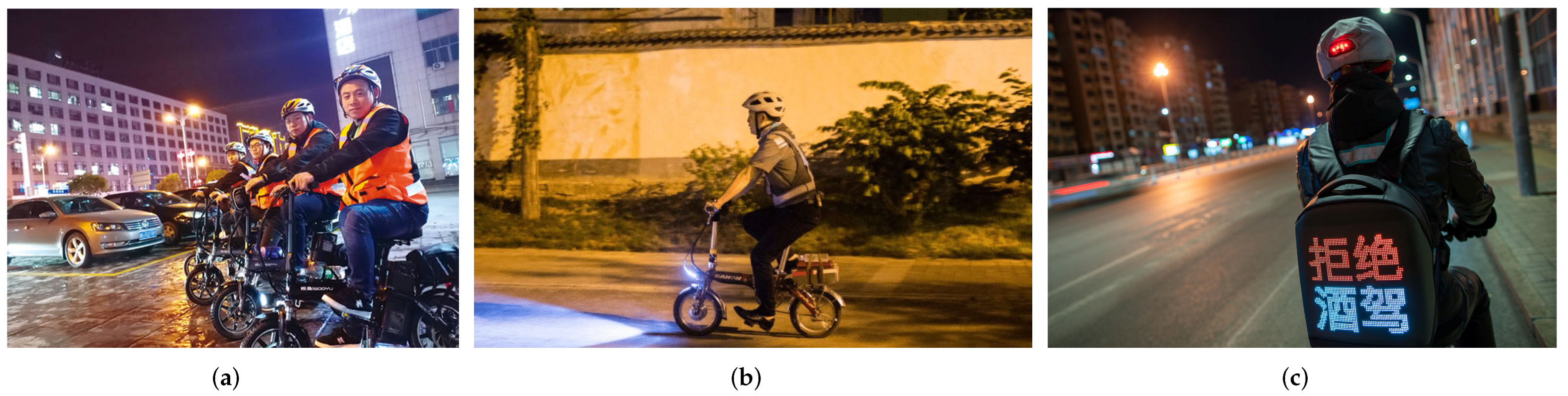Different from the traditional designated driving, which was quite popular among the American general public during the 1980s [1], the valet driver is a part-time laborer and does not have to be one of the cohort attending the festivity. Aside from avoiding driving under the influence (DUI), other situations also exist where the owner of the vehicle cannot drive for herself. For instance, the owner does not know how to operate the vehicle, or the owner is not somewhere near her vehicle and needs it delivered to her. Recently, it has been observed that the soaring amount of demand in the valet driving market has given rise to several valet driving platforms, such as DIDI valet driving and E-valet driving, on which the valet driving orders can be released and matched with the valet drivers. As is shown in Figure 1, the valet driver usually wears a reflective vest and a helmet, rides on a foldable e-bike, and waits for an order assignment outside major restaurants or conference centers.

In fact, valet driving could not only help reduce the number of traffic accidents, but also create more job opportunities in the service industry. Rivara et al. [2] investigated the drinking and driving habits recorded in people aged 21 to 34, and it was reported that 21% of the sampled subjects had the experience of driving after drinking too much in the previous month. This result rings a bell for society, as the percentage of DUI is much higher than was expected; the behavior could cause detrimental effects on the driver as well as victims. Chung et al. [3] investigated the impact of designated driver services on drunk driving behaviors. It was found that an increase in designated driving firms significantly reduced both alcohol-involved and total traffic fatality rates. In addition to reducing traffic accidents, valet driving can also help alleviate employment issues in large cities. Most of the valets are gig workers, and they can serve as designated drivers any time after work, which matches the freelance style of the younger generation. In particular, nonstandard employment relations, such as part-time work, have become increasingly popular [4]. Part-time work is an widely accepted common strategy for balancing work and family [5]. In terms of social welfare, working part-time is potentially beneficial for handling work–life conflicts and makes life easier for parents of young children [6].

Figure 1. Snapshots for valet driving in practice. (a) Waiting for valet orders [7]. (b) Riding to the customer [8]. (c) Say no to DUI [9].

Figure 1. Snapshots for valet driving in practice. (a) Waiting for valet orders [7]. (b) Riding to the customer [8]. (c) Say no to DUI [9].

At present, as more people are enjoying valet driving services, it is necessary for the platforms to respond swiftly to customer requests and to have better capability for driver scheduling. In the valet driving related literature, the focus is on the public belief as to whether they accept the service. To answer the question, a nationwide study was conducted to learn the willingness to use designated drivers by United States college students [10]. Phan et al. [11] made an initial attempt to evaluate the public view toward the designated driving service in Vietnam. More recently, Jou and Syu [12] investigated the willingness of drunk drivers to use and pay for a designated driving service. From a demographic perspective, Timmerman et al. [13] investigated the effects of group size and gender on the recognition of designated driving. As safety is a major concern when using valet driving, Rothe and Carroll [14] explored the risk in the practice of young designated drivers transporting drunken peers. As a marketing probe, Bergen et al. [15] analyzed the characteristics of designated drivers and their passengers from a 2007 national roadside survey in the United States. Based on the above valet driving related literature, it is observed that the existing research work is mostly taken from a more macro viewpoint.

To the best of our knowledge, crew scheduling in the online valet driving problem is largely untouched territory. However, researching crew scheduling in the valet driving problem is crucial, for several reasons. First, as the price of valet driving services remains relatively high, many people are reluctant to use them. This reluctance leads to an increase in drunk driving incidents that often result in serious accidents and injuries. Second, as legal and safety awareness around drunk driving increases, more and more people are beginning to use valet driving services. As the number of drivers and platforms offering these services grows, efficient crew scheduling becomes increasingly important to ensure that customers have access to reliable and timely service.

Given the importance of this issue, we conducted research and proposed a targeted B&P algorithm to solve it. This algorithm can obtain the exact optimal solution of SVDP in a short time, which can effectively improve the scheduling efficiency of the platform for valet drivers and bring multiple benefits in many aspects. Efficient scheduling allows the platform to make better use of their available valet drivers, resulting in increased profits for the platform. Additionally, well-scheduled valets are able to complete more orders within a given time period, increasing their earnings. Furthermore, improved scheduling efficiency translates into lower service costs for customers, making the service more accessible and reducing incidents of drunk driving. As the popularity of valet driving services grows, the industry will create new job opportunities, providing additional benefits to society beyond those noted above.

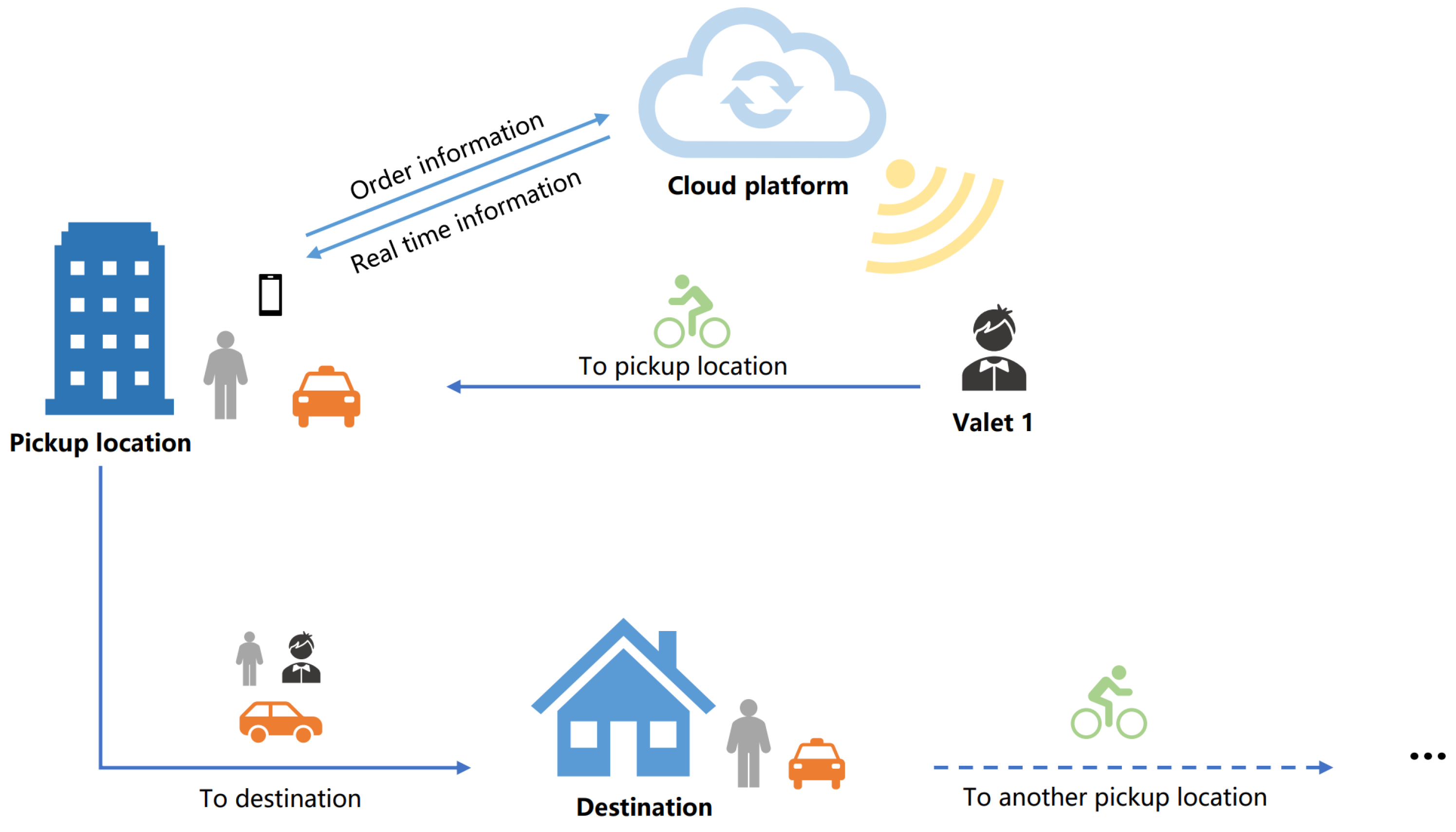
In order to better understand the crew scheduling in the online valet driving problem, we first demonstrate the general process of the valet driving service in Figure 2. The customer, a gray figurine, calls for the valet driving service on the cloud platform through a mobile app. After placing the order, the platform will assign a driver, the black figure, to provide the valet driving service at the designated place. After arrival on an e-bike, the valet puts the foldable e-bike in the trunk of the customer’s vehicle and then drives the customer to her destination. Upon completing the valet driving service, the valet driver continues to ride to the next customer for service.

We summarize the novelty of this paper as follows:

• In the present paper, we investigate the crew scheduling in the online valet driving problem (OVDP), which has not been previously studied. The objective of the OVDP is to minimize the total cost while maintaining a certain quality of service. To denote the service quality, a time window is set for each order to ensure that the customer wait time does not exceed the threshold after placing the order. In addition, all the valet driving requests have to be fulfilled. As the valet rides a foldable e-bike while not driving vehicles, the power level of the e-bike should be considered in the OVDP problem.
• We provide a feasible scheduling strategy for the OVDP problem, which decomposes the OVDP into multiple static valet driving problems (SVDP).
• We devise a feasible modeling scheme for crew scheduling in the SVDP and formulate a mixed integer linear programming (MILP) model to address the corresponding problem. To solve this problem, we propose an exact branch-and-price (B&P) algorithm. Additionally, we introduce a greedy-based constructive heuristic to efficiently obtain an initial solution and implement an artificial column technique when the initial solution cannot be obtained after branching.
• To verify the effectiveness and efficiency of the algorithm, an extensive numerical analysis is performed. In addition, the findings of the present work not only verify the effects of pooling time and scheduling time on the overall performance of the OVDP, but also serve as a reference for applying the smart crew scheduling strategy of the valet driving platform.

The remainder of the paper is presented as follows. In Section 2, a detailed review of the related literature is performed. In Section 3, the problem statement of the OVDP is introduced, and the arc flow-based MILP model of the SVDP is formulated. Then the arc-flow model is reformulated as a set-partition model, and we introduce the column generation algorithm as well as the label-setting algorithm in Section 4. In Section 5, the branch-and-price algorithm is presented. Section 6 shows the results of the numerical analysis. Finally, Section 7 concludes the paper.

2. Literature Review

In the valet related literature, valet parking takes up the largest percentage of research work. Although valet driving is a field receiving more and more attention, another variant of the valet driving, i.e., valet charging, is considered as well. In the field of electric vehicles (EV), Lai and Li [16] proposed a novel business model where a platform provides valet charging services to EV users. After the user places a charging order, the valet responds and picks up the low-power EV from the customer and then drives to a charging station. When the battery is fully charged, the valet drives the EV back to the customer. A queuing network model is constructed to capture the stochastic matching dynamics, and an economic equilibrium model is introduced to justify the incentives of valets, customers, and the platform. The EV charging station location problem was discussed in [17], where the valet charging service was concerned with demand uncertainty. The problem was formulated as a two-stage stochastic mixed-integer model, and a SAA-based hybrid-cut L-shaped algorithm was designed to solve it. The similarity between the above studies and the present research is that we both focus on the valet, and the platforms both need to schedule a cohort of valets. However, the crew scheduling was not considered in the valet charging related papers.

To the best of our knowledge, there are hardly any papers exploring crew scheduling in the online valet driving problem. Thus, other types of crew scheduling literature are included for an inclusive review. Within the literature on the topic of crew scheduling, it is observed that airline crew scheduling is the most covered topic. In [18], the airline crew pairing optimization problem was investigated, and an algorithm based on a combination of column and cut generation was employed. As for the crew and vehicle scheduling, the schedules of vehicle and crew were to be determined simultaneously in order to satisfy a given set of trips over time. Horváth and Kis [19] considered a multi-depot vehicle and crew scheduling problem and constructed a novel mathematical programming model, which is then solved via an exact solution procedure based on branch-and-price. The flexible vehicle and crew scheduling problem faced by urban bus transport was noted in [20]. A MILP model was built and a variable neighborhood search method was used to solve it. At present, the development of EVs is in full swing. Therefore, some scholars also consider the involvement of EVs in the above scenarios. Perumal et al. [21] introduced the integrated EV and crew scheduling problem (E-VCSP) considering with a set of timetabled trips and charging stations. An adaptive large neighborhood search method was introduced together with the branch-and-price algorithm to address the E-VCSP. In addition, there are also some less explored domains with respect to crew scheduling. For example, Duque et al. [22] studied the network repair crew scheduling and routing problem, and it accounted for the emergency repair scheduling of a rural road network, which had been damaged by a natural disaster. To obtain the optimal strategy, an exact dynamic programming (DP) algorithm was used, and an iterated greedy-randomized constructive procedure was integrated as well. The home care crew scheduling problem was addressed in [23], where a group of home carers need to be assigned for visiting the patients’ homes, such that the total service level is maximized.

As a matter of fact, the OVDP problem shares some similarities to the dial-a-ride problem (DARP) to a certain extent. And hence, the literature on the topic of dial-a-ride is reviewed, especially the studies most closely related to the OVDP. The dial-a-ride problem consists of designing vehicle routes and schedules for n users who specify pickup and delivery requests between origins and destinations [24]. Cordeau and Laporte [25] described and classified the primary features of the DARP and discussed the modeling aspects of the problem. The several important algorithms for DARP were summarized. Subsequently, Cordeau and Laporte [24] updated and extended the comprehensive review of the DARP in [25]. More recently, Ho et al. [26] demonstrated the research developments on the dial-a-ride problem and provided classifications of the problem variants as well as the solution methodologies. In addition, several application areas were suggested for the DARP. In

Table 1. Closely related literature on the topic of DARP.

Instance	Ride Time	Time Windows	Working Hours	Non-Selective Visit	Number of Objectives	Power Level	Online with Pooling	Algorithm
[27]	√	√	√	√	S			TS
[28]	√	√	√	√	S			B&C
[29]	√	√	√	√	S			B&C
[30]		√			S			CHA
[31]	√	√	√	√	M			VNS
[32]		√		√	M			GA
[33]	√	√	√	√	S			VNS
[34]				√	S			AA
[35]	√	√		√	S			B&P
[36]		√		√	M			SA
[37]	√	√	√		S			TS
[38]		√	√		M			SA
[39]	√	√	√	√	S			B&C and DA
[40]	√	√		√	S			B&P
[41]	√	√	√		S			B&P
[42]	√	√	√	√	S			B&C&P
[43]	√	√	√	√	S			B&C
[44]	√	√		√	M			VNS
[45]	√	√	√	√	S			HGA
[46]	√	√	√	√	S			ALNS
This study		√		√	S	√	√	B&P

Capacity: loading capacity; TS: tabu search; B&C: branch-and-cut; CH: construction heuristic algorithm; VNS: variable neighborhood search; GA: genetic algorithm; AA: approximation algorithm; B&P: branch-and-price; SA: simulated annealing; DA: deterministic annealing; B&C&P: branch-and-cut-and-price; HGA: hybrid genetic algorithm; ALNS: adaptive large neighborhood search.

, the literature closely related to the DARP in the last twenty years is listed. In the table, the ride time indicates that the study addresses the time customers spent in the ride. Non-selective visit indicates that it is necessary to visit all the customer nodes.

For exact algorithms, to the best of our knowledge, Cordeau [28] was the first to introduce a branch-and-cut algorithm (B&C) for the DARP with three-index mixed integer programming formulation, which applies several families of valid inequalities as cuts. In addition to adopting the identified cuts from Cordeau [28], Ropke et al. [29] introduced three classes of valid inequalities in B&C. Similarly, Braekers et al. [39] and Braekers and Kovacs [43] also employed several valid inequalities to tackle the DARP. In addition to B&C, Garaix et al. [35] introduced the B&P algorithm to handle the DARP, and the pricing subproblem was solved by dynamic programming. By including the time-dependent travel time in the DARP, Hu and Chang [40] developed a B&P algorithm with a heuristic. Parragh et al. [41] developed a B&P algorithm with a hybrid approach for the DARP, and the subproblem was handled via both dynamic programming and heuristics. Taking advantage of both B&C and B&P, Gschwind and Irnich [42] designed a B&P&C algorithm for the DARP and derived an effective column-generation pricing scheme.

In addition to the exact algorithm, heuristic methods and approximation algorithms have been applied to tackle the DARP. The study in [27] was one of the earliest studies applying a tabu search algorithm for the DARP, and the algorithm was shown to be effective and efficient. Inspired by Cordeau and Laporte [27], Kirchler and Calvo [37] proposed a granular tabu search algorithm for the DARP, and Detti et al. [44] integrated variable neighborhood search (VNS) with tabu search algorithm to deal with the more complicated and real-life DARP. In addition, simulated annealing was also used in the literature to solve the DARP, such as in [36,38]. Braekers [39] proposed a new deterministic annealing meta-heuristic for larger-scale DARP. In addition, Parragh et al. [31] developed a variable neighborhood search algorithm for the DARP with two objectives. The same group of authors then introduced a competitive variable neighborhood search-based heuristic [33], which exploits three classes of neighborhoods, to solve the DARP with single objectives. By incorporating the removal operators proposed in [33], Gschwind and Drexl [46] designed an adaptive large neighborhood search method. Based on the adaptation of a generic genetic algorithm model from literature, Cubillos et al. [32] developed a genetic algorithm to solve the DARP with a time window. Masmoudi et al. [45] presented a hybrid genetic algorithm with efficient construction heuristics, crossover operators, and local search techniques. Furthermore, Colvo and Colorni [30] proposed an effective construction heuristic, and Gupta et al. [34] designed approximation algorithms for the DARP.

Compared with the existing literature on the DARP, the online valet driving problem differs from it in three primary aspects. The most distinct feature of the OVDP lies in the fact that it is an online crew scheduling problem with demand pooling, but the DARP is not. Second, the OVDP considers the power level constraint of the valet’s e-bike, whereas the driving in pickup and delivery is homogeneous in the DARP. Finally, because the customer vehicle needs to be driven to the designated location by the valet, the capacity in OVDP is one, unless one can drive more than one vehicle at the same time. In addition, the customer riding time is not considered, given the capacity is one.

3. Problem Description

In this section, we first describe the problem in detail in Section 3.1, including notations and assumptions. We then present the mathematical formulation of the static valet driving problem in Section 3.2.

3.1. Problem Statement

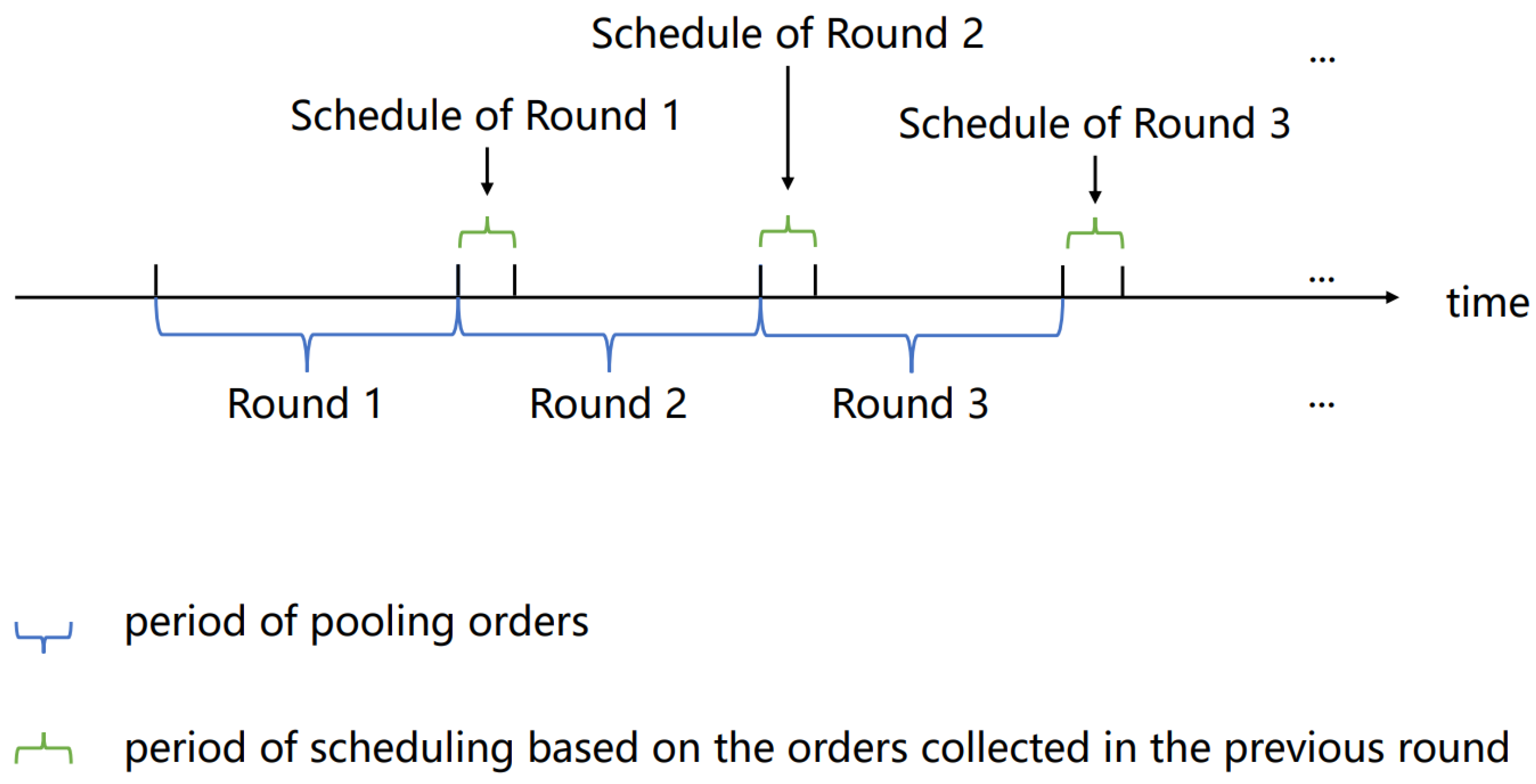
In the online valet driving problem, we discretize the time into time rounds with the same time length. Each round consists of a pooling time and a scheduling time, which is used to collect and schedule orders, respectively. At the end of each pooling time, the scheduling for this round starts, as does the pooling time for the next round. Each round is considered as a static valet driving problem, but the two adjacent rounds are not independent. For example, the position where the valet finishes the task in the previous round will be the initial position of the next round. The relationship among the round, pooling time, and scheduling time is shown in Figure 3.

The SVDP is defined on a directed graph $G=(V,A)$, where $V=\{0,s\}\cup O\cup P\cup D$ is the node set and $A=A_1\cup A_2\cup A_3\cup A_4$ is the arc set. Nodes 0 and s represent the source node and sink node, respectively, which are both dummy nodes. Every valet must start from the source node and end at the sink node. Let set K be the set of valets, $K=\{1,2,\dots ,k\}$. The node mapping function is defined as $o\left(k\right),k\in K$, where $o\left(k\right)$ is the node of the initial location of valet k. The node set O represents the set of the initial locations of the valets, where $O=\left\{o\right(1),o(2),\dots ,o(k\left)\right\}$. The node set P stands for the set of pickup nodes, where $P=\{1,2,\dots ,n\}$ customers are all waiting for service at the pickup nodes. The node set D indicates the set of delivery nodes, where $D=\{n+1,n+2,\dots ,2n\}$ are specified destinations. In addition, the pickup and delivery nodes appear in pairs, such as node i and node $n+i$ for the order i. The arc set $A_1$ represents the arcs from source node to the valets’ initial nodes, which are virtual arcs, where $A_1=\left\{(0,j)\right|j\in O\}$. The arc set $A_2$ stands for the arcs from valets’ initial nodes to pickup nodes or sink node, where $A_2=\left\{(i,j)\right|i\in O,j\in P\cup \left\{s\right\}\}$. For pickup and delivery, the arc set $A_3$ contains the arcs from pickup nodes to the corresponding delivery nodes, where $A_3=\left\{(i,j)\right|i\in P,j=i+n\}$. Similarly, the arc set $A_4$ includes the arcs from delivery nodes to the next pickup nodes or sink node, where $A_4=\left\{(i,j)\right|i\in D,j\in P\cup s,j\ne i-n\}$. Because the valet could be scheduled multiple times, the available time $T_i$ of each valet i needs to be checked before the scheduling starts in each round. To improve the system service level, it is assumed that the customer needs to be served within a certain time window after placing an order. A time window $[e_i,l_i]$ is imposed on each pickup node, where $e_i$ and $l_i$ denote the earliest and the latest time allowed to serve the order i, respectively. The expression $t_{ij}$ indicates the travel time on arc $(i,j)$, and $h_{ij}$ indicates the power consumption on arc $(i,j)$. In addition, it is assumed that the valet’s e-bike has a power level limit, which means that the valet can no longer take orders when the battery depletes.

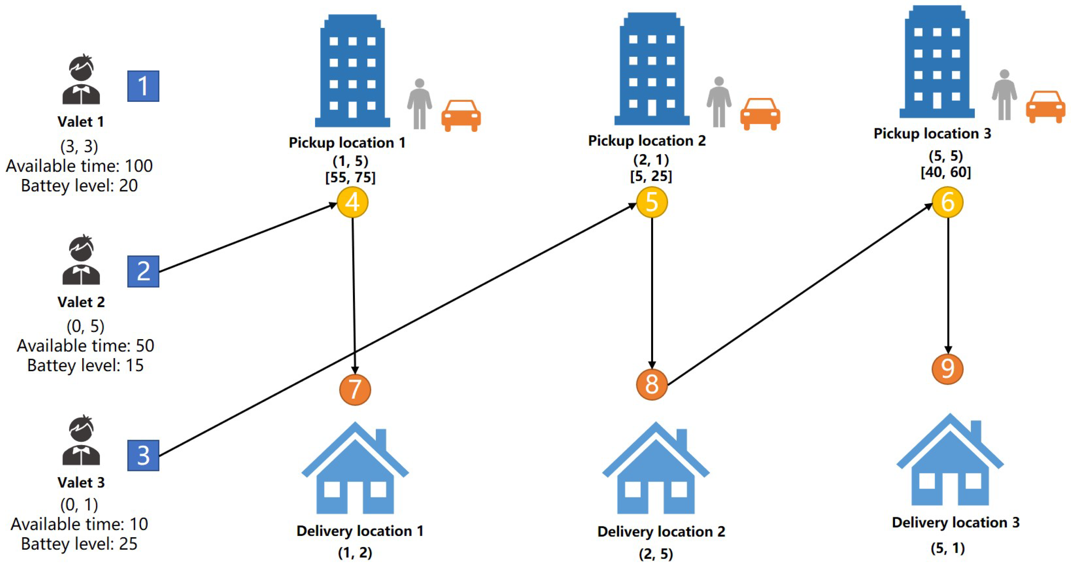
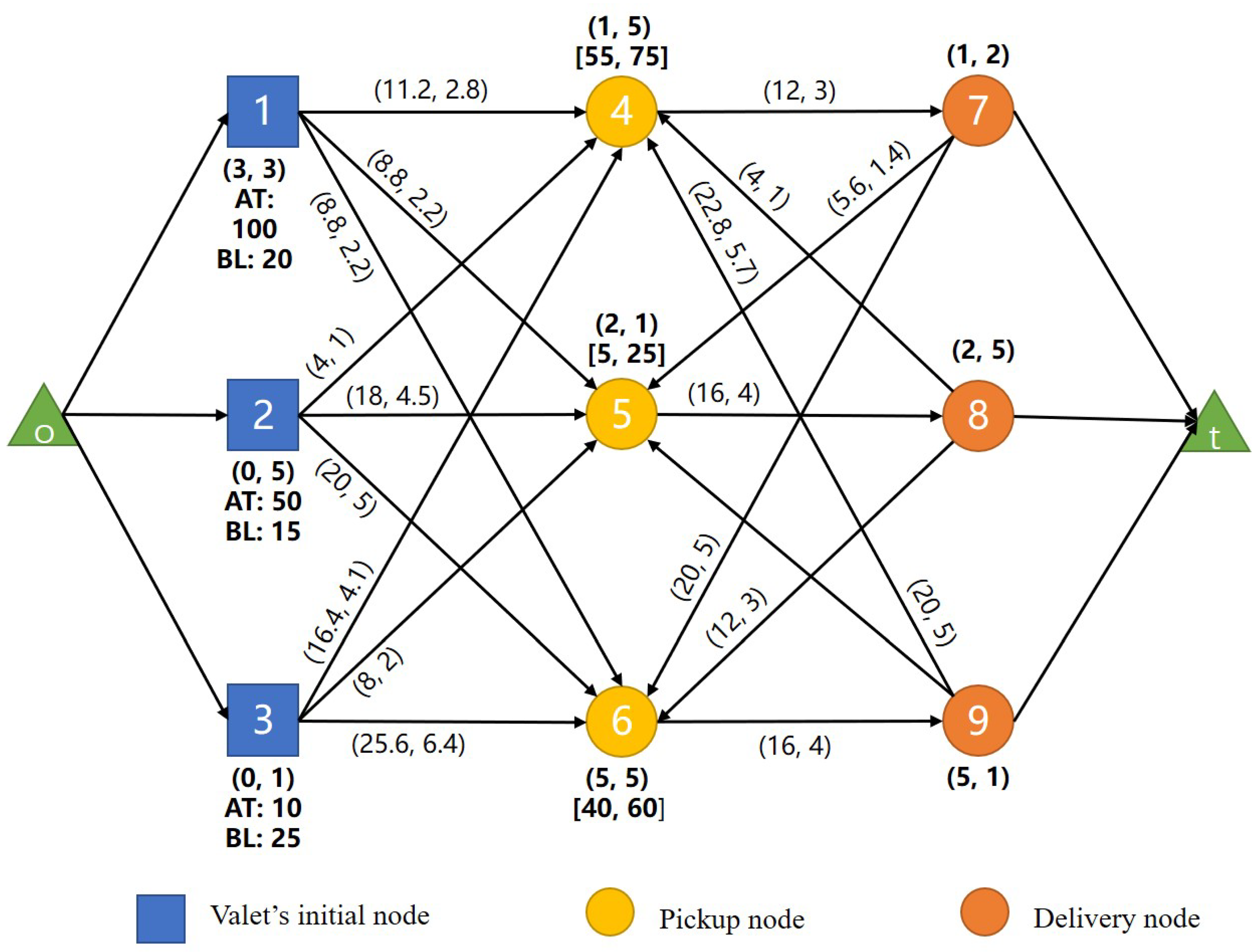
For better understanding, we provide an example of SVDP, as shown in Figure 4. In this example, there are three valets and three orders. Nodes 1, 2, and 3 are the initial nodes of each valet. Nodes 4, 5, and 6 are the pickup nodes of each order. Nodes 7, 8, and 9 are the delivery nodes of each order. Because the source node and sink node are virtual nodes, they do not appear in Figure 4. In addition, “Available Time” represents the time when the valet will complete the current task and become available for the next task. “Battery level” refers to the remaining mileage of the valet’s e-bike. The information in parentheses, such as (1, 5), represents the coordinates of the node, whereas the information in brackets, such as [55, 75], represents the time window of the node. Figure 5 shows the corresponding directed graph for this example, where “AT” represents “Available Time” and “TW” represents time window. 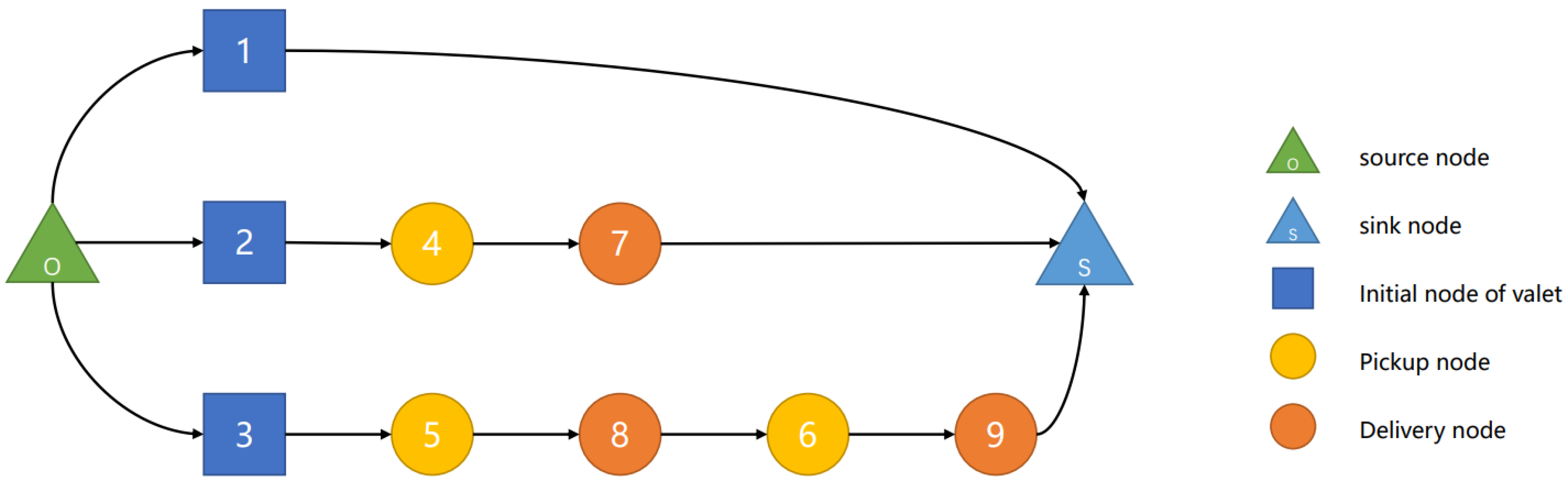In addition, the coordinates and time windows of the nodes are labeled next to the nodes in the same way as in Figure 4. The information in parentheses on the arcs, such as (4, 1), indicates that the first number represents the travel time or cost of the arc, whereas the second number represents the battery consumption of the valet’s e-bike when passing through the arc. The optimal solution for this example is shown in Figure 6.

3.2. Arc-Flow Formulation

In this section, the arc-flow model for the SVDP is introduced. There are three kinds of decision variables in the model: (i) a binary variable $x_{ij}^k$, $x_{ij}^k=1$ if valet k traverses arc $(i,j)$, and 0 otherwise; (ii) a continuous variable $a_i$ that represents the arrival time of node i, $i\in O\cup P\cup D$; (iii) a continuous variable $B_i$ that represents the remaining battery power at node i, $i\in P\cup D$. Note that $B_{o\left(k\right)}$, $k\in K$ is a known parameter, which indicates the initial battery power level at the valet’ initial location. For ease of understanding, we list all the symbols used here in

Table 2. The definition of symbols.

Symbol	Definition
n	The number of customers (orders)
K	Set of valets $K=\{1,2,\dots ,k\}$
P	Set of pickup nodes $P=\{1,2,\dots ,n\}$
D	Set of delivery nodes $D=\{n+1,n+2,\dots ,2n\}$
$o\left(k\right)$	The initial node of valet k
O	The set of initial nodes of valets, $O=\left\{o\right(1),o(2),\dots ,o(k\left)\right\}$
0	Source node
s	Sink node
$A_1$	Set of arcs, $A_1=\left\{(0,j)\right|j\in O\}$
$A_2$	Set of arcs, $A_2=\left\{(i,j)\right|i\in O,j\in P\cup \left\{s\right\}\}$
$A_3$	Set of arcs, $A_3=\left\{(i,j)\right|i\in P,j=i+n\}$
$A_4$	Set of arcs, $A_4=\left\{(i,j)\right|i\in D,j\in P\cup \left\{s\right\},j\ne i-n\}$
A	Set of all arcs, $A=A_1\cup A_2\cup A_3\cup A_4$
$T_i$	Available time of each valet i
$a_i$	Arrival time of node i
$t_{ij}$	Travel time of arc $(i,j)$
$h_{ij}$	Power consumption on arc $(i,j)$
$c_{ij}$	The cost of arc $(i,j)$
$B_i$	Battery power level at node i
$[e_i,l_i]$	Time window of order i

.

$$\begin{array}{cc}\hfill & Min\sum _{k\in K}\sum _{(i,j)\in A}{c}_{ij}{x}_{ij}^k\hfill \end{array}$$

(1)

s.t.

$$\begin{array}{cc}\hfill x_{0,o\left(k\right)}^k& =1,\forall k\in K\hfill \end{array}$$

(2)

$$\begin{array}{cc}\hfill \sum _{k\in K}\sum _{i\in o\left(k\right)\cup D,i\ne j+n}{x}_{ij}^k& =1,\forall j\in P\hfill \end{array}$$

(3)

$$\begin{array}{cc}\hfill \sum _{j\in P\cup \left\{s\right\}}{x}_{o\left(k\right),j}^k& =1,\forall k\in K\hfill \end{array}$$

(4)

$$\begin{array}{cc}\hfill x_{i,i+n}^k-\sum _{j\in D\cup \left\{o\right(k\left)\right\},j\ne i+n}{x}_{ji}^k& =0,\forall k\in K,i\in P\hfill \end{array}$$

(5)

$$\begin{array}{cc}\hfill x_{i-n,i}^k-\sum _{j\in P\cup \left\{s\right\},j\ne i-n}{x}_{ij}^k& =0,\forall k\in K,i\in D\hfill \end{array}$$

(6)

$$\begin{array}{cc}\hfill \sum _{i\in D}{x}_{is}^k+x_{o\left(k\right),s}^k& =1,\forall k\in K\hfill \end{array}$$

(7)

$$\begin{array}{cc}\hfill a_{o\left(k\right)}& \ge T_{o\left(k\right)},\forall k\in K\hfill \end{array}$$

(8)

$$\begin{array}{cc}\hfill x_{ij}^k=1\Rightarrow a_j& \ge a_i+t_{ij},\forall k\in K,(i,j)\in A,j\ne s\hfill \end{array}$$

(9)

$$\begin{array}{cc}\hfill e_i\le a_i& \le l_i,\forall i\in P\hfill \end{array}$$

(10)

$$\begin{array}{cc}\hfill x_{ij}^k=1\Rightarrow B_j& =B_{o\left(k\right)}-h_{ij},\forall k\in K,(i,j)\in A_2\hfill \end{array}$$

(11)

$$\begin{array}{cc}\hfill x_{ij}^k=1\Rightarrow B_i& =B_j,\forall k\in K,(i,j)\in A_3\hfill \end{array}$$

(12)

$$\begin{array}{cc}\hfill x_{ij}^k=1\Rightarrow B_j& =B_i-h_{ij},\forall k\in K,(i,j)\in A_4\hfill \end{array}$$

(13)

$$\begin{array}{cc}\hfill x_{ij}^k& \in \{0,1\},\forall k\in K,(i,j)\in A\hfill \end{array}$$

(14)

$$\begin{array}{cc}\hfill a_i& \ge 0,i\in O\cup P\cup D\hfill \end{array}$$

(15)

$$\begin{array}{cc}\hfill B_i& \ge 0,i\in P\cup D\hfill \end{array}$$

(16)

The objective Function (1) is to minimize the total cost, which is the sum of costs on all the traversed arcs. A smaller total cost means a higher utilization rate of valets and better scheduling results. Constraint (2) ensures that each valet must reach its initial node from the source node through a virtual path, in order to maintain consistency with the path set model generated in Section 4.1. The order nodes visited after that initial node represent the orders completed by the valet corresponding to that initial node. Constraint (3) states that the indegree of each pickup node is 1, and the previous node must be either the valet’s initial node or another order’s delivery node. This ensures that each pickup node is visited only once, meaning each order must be completed. Constraint (4) implies that after departing from an initial node, the valet can only travel to a pickup node or return to the sink node. If the valet travels to a pickup node, it means that the valet has been assigned an order; if the valet directly returns to the sink node, it means that the valet has not been assigned any orders. Constraints (5) and (6) are flow balance constraints for pickup nodes and delivery nodes, respectively, which means that the indegree of each node equals its outdegree. Constraint (7) ensures that each valet must return to the sink node, and once a valet returns to the sink node, it means that all tasks assigned to him or her have been completed. Constraint (8) indicates that each valet can only depart from his or her initial node after entering the idle state. Constraint (9) establishes the relationship between the arrival times of a valet at two consecutive nodes, meaning that the visit time of the latter node must be greater than or equal to the visit time of the former node plus the time required for the journey in between. Constraint (10) is the time window constraint for each order, meaning that the node can only be visited within the specified time window. Constraints (11)–(13) establish the relationship between the battery level of a valet when visiting two consecutive nodes, which means that the remaining range when visiting the latter node is equal to the remaining range when visiting the former node minus the consumed range during the journey in between. Finally, Constraints (14)–(16) define the decision variables.

4. Column Generation-Based Method

Although the arc-flow model in Section 3.2 can be solved via commercial solvers such as Cplex and Gurobi, it is found that the computation efficiency of commercial solvers is rather low in the numerical tests. As the OVDP is an online optimization problem in essence, the solving speed is a critical factor to be considered. In order to speed up the solving, we first reformulate the problem as a set partitioning model, namely, the restricted master problem (RMP), which is with only a subset of decision variables (columns). The formulation is described in Section 4.1. The column generation is applied to solve the linear relaxation of RMP, which is called the restricted linear master problem (RLMP). The column generation is an iterative procedure. In each iteration, the RLMP is solved first to reach the dual optimal of the RMP. Then the pricing subproblem is processed with the obtained dual information. If the pricing subproblem can obtain a column with negative reduced cost, the column is added to the RLMP. Finally, the label setting algorithm is implemented to solve the pricing problem to find potential viable columns, which is demonstrated in Section 4.3.

It is worth noting that when adding columns to the RLMP by solving the subproblem, it is not necessary to add all columns with negative reduced cost to the RLMP. Doing so will also lead to a particularly large number of variables in the RLMP during the later stage of solving RLMP, resulting in a slower solving speed. The approach adopted by some scholars is to only add the column with the most negative reduced cost each time. In our testing, however, it was found that adding multiple columns at once would be better. Doing so greatly improves the solving speed. After extensive testing, it was found that adding up to 20 columns at a time is a suitable choice in our problem, and these columns have the 20 most negative reduced costs.

4.1. Set Partition Formulation

Let $\Omega$ be the set of all feasible routes of the valets. Each route $r\in \Omega$ represents a route that starts from the source node and ends at the sink node, and its cost is denoted by $c_r$. The variable $b_{ij}^r$ indicates whether route r traverses through arc $(i,j)$: $b_{ij}^r=1$ means route r traverses thought arc $(i,j)$, otherwise $b_{ij}^r=0$. Variable $a_{ir}$ represents whether node i is visited in route r: $a_{ir}=1$ means node i is visited in the route r, otherwise $a_{ir}=0$. Then, the following relationship $c_r={\sum }_{(i,j)\in A}{b}_{ij}^r{c}_{ij}$, $a_{ir}={\sum }_{\{i\in V|(i,j)\in A\}}{b}_{ij}^r$ is obtained. There is only a binary decision variable ${\theta }_r$ in the set partitioning model; ${\theta }_r$ equals 1 if route r is selected in the solution, and 0 otherwise. There is also a binary parameter $a_{ir}$, which equals 1 if node i is visited in route r, and 0 otherwise.

The set partitioning model is presented as follows:

$$\begin{array}{c}\hfill Min\sum _{r\in \Omega }{c}_r{\theta }_r\end{array}$$

(17)

s.t.

$$\begin{array}{cc}\hfill \sum _{r\in \Omega }{a}_{ir}{\theta }_r=1,& \forall i\in O\cup P\hfill \end{array}$$

(18)

$$\begin{array}{c}\hfill \sum _{r\in \Omega }{\theta }_r\le \left|K\right|\end{array}$$

(19)

The objective Function (17) is to minimize the total cost of all the selected routes. Constraint (18) ensures that each order can only be served once and every valet can only start once. Constraint (19) means that the number of all selected routes is less than or equal to the number of valets.

4.2. Pricing Subproblem

When the scale of the problem is large, the size of $\Omega$ will grow exponentially. Hence it is almost impossible to explicitly represent the set $\Omega$. However, the RMP can be obtained by considering a subset of paths $\overline{\Omega }\subseteq \Omega$ in each iteration. The function of the pricing subproblem is to generate feasible paths (column) with negative reduced cost, which have the potential to reduce the value of the objective function. Then, we can add the generated paths to $\overline{\Omega }$ iteratively. We let ${\lambda }_i,i\in O\cup P$ represent the dual variables associated with Constraint (18). There are $\left|O\right|+\left|P\right|$ variables of ${\lambda }_i$ in total. Let ${\lambda }_0$ be the dual variable associated with Constraint (19).

The reduced cost of route $r\in \Omega$ is derived as follows:

$$\begin{array}{c}\hfill \overline{c_r}=c_r-\sum _{i\in O\cup P}{a}_{ir}{\lambda }_i-{\lambda }_0\end{array}$$

(20)

In fact, the pricing subproblem is in essence an elementary shortest path problem with resource constraints (ESPPRC), and it can be defined as below:

$$\begin{array}{c}\hfill min{c}_r-\sum _{i\in O\cup P}{a}_{ir}{\lambda }_i-{\lambda }_0\end{array}$$

(21)

According to $c_r={\sum }_{(i,j)\in A}{b}_{ij}^r{c}_{ij}$, $a_{ir}={\sum }_{i\in V}{b}_{ij}^r$, Formula (21) can be rewritten as

$$\begin{array}{c}\hfill min\sum _{(i,j)\in A}{b}_{ij}^r{c}_{ij}-\sum _{\{i\in O\cup P|(i,j)\in A\}}{b}_{ij}^r{\lambda }_i-{\lambda }_0\end{array}$$

(22)

Then, Formula (22) can be further illustrated as

$$\begin{array}{c}\hfill min\sum _{(i,j)\in A\setminus A_4}{b}_{ij}^r(c_{ij}-{\lambda }_i)+\sum _{(i,j)\in A_4}{b}_{ij}^r{c}_{ij}\end{array}$$

(23)

Finally, Formula (23) can be succinctly expressed as

$$\begin{array}{c}\hfill min\sum _{(i,j)\in A}{b}_{ij}^r\overline{c_{ij}}\end{array}$$

(24)

Let $x_{ij}$ indicate whether to access arc $(i,j)$: $x_{ij}=1$ represents that arc $(i,j)$ is traversed, otherwise $x_{ij}=0$. Then the pricing subproblem can be specifically formulated in the following form:

$$\begin{array}{c}\hfill Min\sum _{(i,j)\in A}\overline{c_{ij}}{x}_{ij}\end{array}$$

(25)

s.t.

$$\begin{array}{cc}\hfill \sum _{i\in O}{x}_{0,i}& =1\hfill \end{array}$$

(26)

$$\begin{array}{cc}\hfill \sum _{j\in P\cup \left\{s\right\}}{x}_{ij}& =1,\forall i\in O\hfill \end{array}$$

(27)

$$\begin{array}{cc}\hfill x_{i,i+n}-\sum _{j\in D\cup O,j\ne i+n}{x}_{ji}& =0,\forall i\in P\hfill \end{array}$$

(28)

$$\begin{array}{cc}\hfill x_{i-n,i}-\sum _{j\in P\cup \left\{s\right\},j\ne i-n}{x}_{ij}& =0,\forall i\in D\hfill \end{array}$$

(29)

$$\begin{array}{cc}\hfill \sum _{i\in O\cup D}{x}_{is}& =1\hfill \end{array}$$

(30)

$$\begin{array}{cc}\hfill a_i& \ge T_i,\forall i\in O\hfill \end{array}$$

(31)

$$\begin{array}{cc}\hfill x_{ij}=1\Rightarrow a_j& \ge a_i+t_{ij},\forall (i,j)\in A,j\ne s\hfill \end{array}$$

(32)

$$\begin{array}{cc}\hfill e_i\le a_i& \le l_i,\forall i\in P\hfill \end{array}$$

(33)

$$\begin{array}{cc}\hfill x_{ij}=1\Rightarrow B_j& =B_i-h_{ij},\forall (i,j)\in A_2\cup A_4\hfill \end{array}$$

(34)

$$\begin{array}{cc}\hfill x_{ij}=1\Rightarrow B_i& =B_j,\forall (i,j)\in A_3\hfill \end{array}$$

(35)

$$\begin{array}{cc}\hfill x_{ij}& \in \{0,1\},\forall (i,j)\in A\hfill \end{array}$$

(36)

$$\begin{array}{cc}\hfill a_i& \ge 0,i\in O\cup P\cup D\hfill \end{array}$$

(37)

$$\begin{array}{cc}\hfill B_i& \ge 0,i\in P\cup D\hfill \end{array}$$

(38)

4.3. Label Setting Algorithm

The purpose of solving ESPPRC is to find the path with the minimum reduced cost; however, the ESPPRC is itself proved to be NP-hard. At present, the label setting algorithm is often employed to search for feasible paths with negative reduced cost to for the ESPPRC. Therefore, we also design a label setting algorithm for our problem. In general, the label setting algorithm starts with one or several initial labels and then extends those labels according to extension rules. Although all feasible paths can be enumerated through the label setting algorithm, the number of feasible paths is huge, making the process time-consuming. Therefore, exhaustive enumerations are avoided with tailored techniques, such as dominance rules, which narrow down the search scope to only the effective paths. Dominance rules can be regarded as an acceleration technology, which is able to discard the low-quality routes in the process of extension and ensures that the optimal path is not discarded. The details of the label setting algorithm with dominance rules used in the present paper are described as follows.

In the label setting algorithm proposed here, each label contains five attributes: $L_i=\{{\eta }_i,c_i^{\prime },A_i,p_i,C_i,L_i^{*}\}$ is defined as a label corresponding to the partial path, which starts from the source node to node ${\eta }_i$. The meaning of each attributes in label $L_i$ is shown as below:

• ${\eta }_i$: the last node of the partial path;
• $c_i^{\prime }$: the accumulated reduced cost of the partial path, including travel cost between source node and node ${\eta }_i$ and associated dual variable value;
• $A_i$: arrival time at the last node;
• $p_i$: the remaining power of the battery when the valet arrives at node ${\eta }_i$;
• $C_i$: the set of visited nodes in the partial path;
• $L_i^{*}$: the parent label of the current label.

4.3.1. Initialization

The label setting algorithm is initialized with a unique label $L_0$ at the source node, which is defined as, ${\eta }_0=0$, $c_0^{\prime }=0$, $A_0=0$, $p_0=null$, $C_0=\varnothing$, and, as it has no parent label, we have $L_0=\{0,0,0,null,\varnothing ,null\}$.

4.3.2. Extension

The extension rules are described in detail as follows. A label $L_1$ at node i can extend to another label $L_2$ at node j along the arc $(i,j)$. There are four different types of extension; the specific extension cases and the label update methods are described below.

The unique initial label can only be extended to node $o\left(k\right),k\in K$ along arc $(0,o\left(k\right))\in A_1$, and the attributes of the new label $L_j$ are shown as follows: ${\eta }_j=o\left(k\right)$, $c_j^{\prime }=c_{0,o\left(k\right)}-{\lambda }_0=-{\lambda }_0$, $A_j=T_{o\left(k\right)}$, $p_j=B_{o\left(k\right)}$, $C_j=\varnothing$, and $L_j^{*}=L_0$.

When extending label $L_i$ from node ${\eta }_i\in O$ to a pickup node p, the extension is feasible if it satisfies the following conditions:

$$\begin{array}{c}\hfill p\notin C_i\\ \hfill A_i+t_{{\eta }_i,p}\le l_p\\ \hfill p_j\ge h_{{\eta }_i,p}\end{array}$$

and then the new label $L_j$ updates as ${\eta }_j=p$, $c_j^{\prime }=c_i^{\prime }+c_{{\eta }_i,p}-{\lambda }_{{\eta }_i}$, $A_j=max\{A_i+t_{{\eta }_i,p},a_p\}$, $p_j=p_i-h_{{\eta }_i,p}$, $C_j=C_i\cup \left\{p\right\}$, and $L_j^{*}=L_i$. Similarly, when extending label $L_i$ from node ${\eta }_i\in D$ to a pickup node p, the extension is feasible if it meets the above conditions. The updated label $L_j$ is the same as the above case, except that $c_j^{\prime }=c_i^{\prime }+c_{{\eta }_i,p}$.

A label $L_i$ from node ${\eta }_i\in P$ must extend to its corresponding delivery node p, where $p={\eta }_i+n$, and the new label $L_j$ updates as ${\eta }_j=p$, $c_j^{\prime }=c_i^{\prime }+c_{{\eta }_i,p}-{\lambda }_{{\eta }_i}$, $A_j=A_i+t_{{\eta }_i,p}$, $p_j=p_i$, $C_j=C_i$, and $L_j^{*}=L_i$.

4.3.3. Dominance Rule

Considering two labels $L_k$ and $L_{k^{\prime }}$ at the same node, e.g., ${\eta }_k={\eta }_{k^{\prime }}$, $L_k$ dominates $L_{k^{\prime }}$ if the following inequalities hold, and at least one is strict:

• $c_k^{\prime }\le c_{k^{\prime }}^{\prime }$;
• $A_k\le A_{k^{\prime }}$;
• $p_k\ge p_{k^{\prime }}$;
• $C_k\subseteq C_{k^{\prime }}$.

Applying this dominance rule will effectively reduce the number of labels, increase the efficiency of the algorithm, and ensure that the labels with respect to the optimal path are not discarded in the process. The validity and the correctness of the dominance rule is demonstrated in the following lemma.

Lemma 1.

Let label $L_1$ dominate label $L_2$, and let $L_4$ be an extended label of $L_2$. Then, there exists a label $L_3$ extended from $L_1$ that dominates label $L_4$.

Proof.

Suppose a label $L_1=\{{\eta }_1,c_1^{\prime },T_1,p_1,C_1,L_1^{*}\}$ and a label $L_2=\{{\eta }_2,c_2^{\prime },T_2,p_2,C_2,L_2^{*}\}$. Let $L_4$ be an extended label from $L_2$ to a node k. Without loss of generality, let us assume that $L_1$ and $L_2$ are associated with the delivery node d, i.e., ${\eta }_1={\eta }_2=d$, and node k is a pickup node. According to the dominance rule, we have $c_1^{\prime }\le c_2^{\prime }$, $T_1\le T_2$, $p_1\ge p_2$, and $C_1\subseteq C_2$. Then, considering a label $L_3$ extended from $L_1$ to node k, we have $c_3^{\prime }=c_1^{\prime }+c_{dk}-{\lambda }_h$, $c_4^{\prime }=c_2^{\prime }+c_{dk}-{\lambda }_h$, hence we have $c_3^{\prime }\le c_4^{\prime }$; $T_3=T_1+t_{dk}$, $T_4=T_2+t_{dk}$, thus $T_3\le T_4$; $p_3=p_1-h_{dk}$, $p_4=p_2-h_{dk}$, thus $p_3\ge p_4$; $C_3=C_1\cup \left\{k\right\}$, $C_4=C_2\cup \left\{k\right\}$, hence we have $C_3\subseteq C_4$. In summary, we have the conclusion that $L_3$ dominates $L_4$.    □

4.4. Heuristic Pricing

During the initial testing of the algorithm performance, it was found that the time to solve the RLMP on each node is very short. In comparison, it is time-consuming to apply the label setting algorithm to solve the pricing subproblems for negative columns. Because all feasible extensions will be traversed and all negative columns will be found during the complete execution of the label algorithm, the label setting algorithm takes a long time when the problem is large in scale. However, it is not necessary to find all negative columns each time. For most of the time, it is enough to only find the relatively negative columns. Therefore, the heuristic pricing algorithm is adopted to accelerate the solving of the pricing subproblem. Therefore, we refer to the truncated labeling algorithm as noted in [47]. In this truncated labeling algorithm, only a limited number of labels are stored in each node. Based on the results of the numerical experiments, it is found that the acceleration effect is relatively good when the number of labels is set to 50. When solving the pricing subproblem, the heuristic pricing algorithm will be implemented first. When the heuristic pricing algorithm cannot find any negative column, the label setting algorithm will be initiated to search for all the negative columns.

5. Branch-and-Price Algorithm

The branch-and-price algorithm (B&P) is composed of branch-and-bound and column generation, and the column generation procedure is implemented to the RLMP at each branch-and-bound node. If the solution of the RLMP is integral, it is an upper bound of the optimal solution. Otherwise, if the solution is fractional, then we need to branch. At each branch-and-bound node, a constructive heuristic is applied to obtain an initial solution. If the heuristic fails to obtain any initial solution, then an artificial column is added to ensure that the column generation procedure can be implemented. 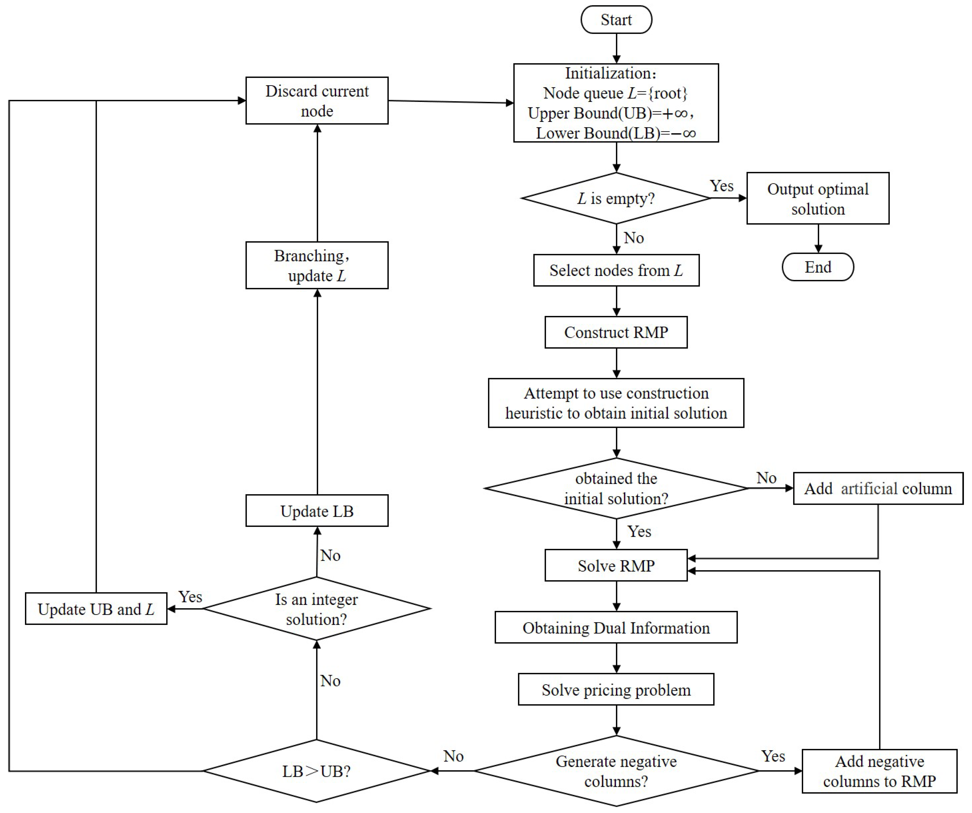The details of the constructive heuristic are presented in Section 5.1, and the procedure of including the artificial column is described in Section 5.3. Here, we first provide a schematic diagram of our proposed B&P algorithm, as shown in Figure 7.

5.1. Initial Solution

In order to obtain an initial solution quickly so as to facilitate the subsequent implementation of the column generation, a constructive heuristic based on greedy search is designed. The detailed steps of this heuristic are described as follows. First, the orders are sorted in non-decreasing order according to the left time window. Then the sorted orders are sent to valets in sequence. The general rule is to assign each order to the valet who is closest to the pickup node of the order, without violating the time window and power level constraints. After assigning the order to the valet, the pickup and delivery nodes of the order are added to the path of the valet in turn. Next, the location, the battery power level, and available time of the valet are updated. Finally, the above order assignment procedure is repeated until all the orders are assigned. The pseudo-code of this heuristic is demonstrated in Algorithm 1. In addition, the same heuristic is also employed to obtain initial solutions for the branch-and-bound nodes.

Algorithm 1 Greedy based constructive heuristic.

Input: orderList O, valetList V 1: Initialization: For every valet $v\in V$, add the source node and the valet initial node to the path $P_v$; 2: for each order $o\in O$ do 3:     According to the information of o and V, find the nearest available valet k; 4:     Add the pickup node and delivery node of order o in the path $P_k$ of valet k; 5:     Update the location, battery power level, and available time and of the valet k; 6: end for Output: $P_v,v\in V$, valetList V

5.2. Branching Scheme

The best bound strategy is applied to explore the branch-and-bound tree. Through the column generation, the RLMP solution corresponding to each branch-and-round node is obtained, that is, the lower bound of the node. Then priority is given to the branch-and-bound node with the minimum lower bound. When the minimum lower bound meets the upper bound, the optimal solution is obtained, and the algorithm is terminated.

For a branch-and-bound node, let $f_{ij}$ be the flow of arc $(i,j)\in A$, where $f_{ij}={\sum }_{r\in \overline{\Omega }}{a}_{ir}{\theta }_r$. The arc $(i,j)=arg{max}_{\left(\right(i,j)\in A)}\{c_{ij}\times min\{f_{ij},|1-f_{ij}\left|\right\}\}$ is selected to branch. In other words, we choose the arc with the flow closest to 1 or closest to 0 on the arc for branching. In the final optimal integer solution, for each arc in the graph, there are only two possibilities: being accessed once or not being accessed. It is believed that if the flow on an arc approaches 1 in a non-integer solution, it is most likely to appear in the final optimal integer solution. In comparison, if the flow rate on an arc approaches 0, it is the least likely to appear in the final optimal integer solution.

Furthermore, not all the arcs can be selected for branching. In our problem, after the valet driver arrives at a pickup point, he/she can only go to the corresponding delivery point, so there is no need to branch such arcs. The arc $(0,i),i\in O$ also does not require branching, as this is equivalent to the departure process of valet drivers. In our modeling, each valet driver will depart, even if he/she has not been assigned to any order, but in this case, he/she will directly return to the sink node. Therefore, in our branching strategy, only the arc $(i,j)\in A_2\cup A_4$ needs to be branched.

After branching, for one child node, we let $f_{ij}=0$, which means that the arc cannot be in the path as part of the solution. Thus, we need to let $x_r=0$ for all the paths containing arc $(i,j)$. The other child node satisfies $f_{ij}=1$, which means the arc is contained in the solution.

5.3. Artificial Column

When branching a node, it is possible that several columns are prohibited, and the remaining columns on the child nodes are insufficient to generate a feasible solution. At this time, the constructive heuristic introduced in Section 5.1 is applied to generate a feasible solution. If it still fails to obtain a feasible solution, an artificial column is added to that node, where it is assumed that a valet completes all the orders. This virtual path starts from the source node, then goes to the initial valet node, visits the pickup and delivery nodes of all the orders, and finally ends at the sink node. It is noticeable that this artificial column corresponds to a path that is not feasible in reality. Thus the cost of this virtual path is set to be a large number. In this way, this node can obtain an initial solution with huge penalty cost, but the subsequent column generation can be implemented. If the node has a feasible solution, the virtual solution is disregarded by default, because the objective function value of the feasible solution must be smaller than the virtual solution. If the node has no feasible solution, the node is also pruned, as its objective function value is larger than the upper bound. Therefore, adding artificial column does not rule out the optimal solution.

6. Computational Experiments

In this section, we conduct a series of numerical experiments to test the performance of the proposed B&P algorithm. First of all, the performance of the proposed B&P algorithm is compared with a commercial solver. The experiments are divided into three scales according to the number of valets, namely, small-scale, medium-scale, and large-scale. Then, an in-depth analysis is performed to investigate the impacts of pooling time and scheduling time on the OVDP. The B&P algorithm is implemented in Java, and Cplex version 20.1 is used as the benchmark. The computing platform is a desktop computer equipped with AMD Ryzen${}^{\mathrm{TM}}$ 7 5800 H 3.2 GHz processor, 16 GB RAM, and Windows 10 OS.

6.1. Comparison with Commercial Solver

In the field of operations research, Cplex is a widely used commercial mathematical programming solver. Due to its excellent solving efficiency and accuracy, the Cplex solver is considered one of the most advanced solvers currently available. Many researchers use Cplex to test algorithms and models they have developed and compare their performance with Cplex’s performance as a benchmark. Therefore, in our research, we also use Cplex’s solving performance as a benchmark to test the performance of our proposed algorithm. We input the objective function and constraints of the problem defined in Models (1)–(16) into the Cplex solver by programming. The Cplex solver uses its internal optimization algorithms to find the optimal solution and returns the obtained solution and the time taken to solve it as a benchmark for comparison. Moreover, we can set the maximum solving time. If the global optimal solution is not found within the specified time, the solver will output the current optimal solution and the current gap.

Therefore, in this subsection, we evaluate the performance of the B&P algorithm in comparison with Cplex in small, medium, and large scales. In the experiment, a 30-min online scheduling process of OVDP is simulated. The pooling time is set to be 5 min and the scheduling time is 1 min. The pickup and delivery points are generated randomly for all the orders. The release time for each order is randomly generated between 0 and 30 min. The width of the time window is 15 min, and the left time window is the order release time. The initial positions of all the valets are also generated randomly. The battery power level of the valets’ electric bicycle is generated randomly between 15 and 30 km, and the initial available time of each valet is assumed to be between 0 and 15 min.

For each group of experiments, the ratio of the number of orders and the number of valets is used to reflect the three different order levels. The ratios are 1, 2, and 3, respectively. For small, medium, and large scaled instances, the number of valets is 50, 75, and 100, respectively. The testing results with respect to different scales are demonstrated in

Table 3. Performance comparison for small-scale instances.

	Cplex			B&P
Instance	Obj	Time	CR	Obj	Time	CR	Time-I	Obj-I
	268.4	5.63	6/6	268.4	1.69	6/6	69.98%	0%
	316.7	5.26	6/6	316.7	2.20	6/6	58.17%	0%
50–50	306.2	4.90	6/6	306.2	1.82	6/6	62.86%	0%
	297.2	5.73	6/6	297.2	1.78	6/6	68.94%	0%
	324.9	5.44	6/6	324.9	1.93	6/6	64.52%	0%
	618.9	23.53	6/6	618.9	4.86	6/6	79.37%	0%
	553.4	20.54	6/6	553.4	4.36	6/6	78.77%	0%
50–100	545.6	20.72	6/6	545.6	5.19	6/6	74.95%	0%
	632.5	21.90	6/6	632.5	3.05	6/6	86.07%	0%
	592.3	83.67	6/6	583.2	4.68	6/6	94.41%	1.54%
	-	-	2/6	864.6	9.06	6/6	-	-
	-	-	1/6	872.0	13.87	6/6	-	-
50–150	-	-	1/6	873.6	7.31	6/6	-	-
	-	-	1/6	977.0	8.87	6/6	-	-
	-	-	4/6	883.1	10.42	6/6	-	-

,

Table 4. Performance comparison for medium-scale instances.

	Cplex			B&P
Instance	Obj	Time	CR	Obj	Time	CR	Time-I	Obj-I
	396.6	22.61	6/6	396.6	5.41	6/6	76.09%	0%
	423.7	19.89	6/6	423.7	5.24	6/6	73.66%	0%
75–75	418.3	21.53	6/6	418.3	4.52	6/6	79.01%	0%
	410.1	20.08	6/6	410.1	5.66	6/6	71.81%	0%
	427.4	18.58	6/6	427.4	4.39	6/6	76.37%	0%
	889.4	73.33	6/6	889.4	16.38	6/6	77.66%	0%
	-	-	4/6	899.4	14.98	6/6	-	-
75–150	-	-	5/6	829.7	18.92	6/6	-	-
	798.8	76.41	6/6	798.8	11.17	6/6	85.38%	0%
	913.1	99.12	6/6	913.1	10.14	6/6	89.77%	0%
	-	-	1/6	1260.5	27.34	6/6	-	-
	-	-	0/6	1270.8	51.32	6/6	-	-
75–225	-	-	0/6	1260.8	32.64	6/6	-	-
	-	-	0/6	1372.5	32.93	6/6	-	-
	-	-	0/6	1411.4	20.71	6/6	-	-

and

Table 5. Performance comparison for large-scale instances.

	Cplex			B&P
Instance	Obj	Time	CR	Obj	Time	CR	Time-I	Obj-I
	594.0	38.15	6/6	594.0	14.27	6/6	62.60%	0%
	540.1	36.98	6/6	540.0	10.10	6/6	72.69%	0.02%
100–100	557.9	39.70	6/6	557.9	11.89	6/6	70.05%	0%
	545.0	36.35	6/6	545.0	13.39	6/6	63.16%	0%
	561.6	44.93	6/6	561.6	15.40	6/6	65.72%	0%
	1121.3	218.58	6/6	1114.7	57.65	6/6	73.63%	0.59%
	-	-	5/6	1136.9	26.46	6/6	-	-
100–200	1092.9	174.43	6/6	1092.9	30.21	6/6	82.68%	0%
	-	-	5/6	1102.1	44.44	6/6	-	-
	-	-	1/6	1113.7	32.54	6/6	-	-
	-	-	0/6	-	-	5/6	-	-
	-	-	0/6	1687.4	75.15	6/6	-	-
100–300	-	-	0/6	1698.4	62.47	6/6	-	-
	-	-	0/6	-	-	3/6	-	-
	-	-	0/6	-	-	1/6	-	-

.

For each table, the first column denotes the name of a type of instance. For example, “50–100” means that there are 50 valets and 100 orders in this type of instance, and the ratio of order quantity to valet quantity is 2. For each type, that is, order level, the performance of five instances are recorded. The following six columns present the performance comparison between Cplex and the B&P algorithm. In this experiment, we simulated a 30 min online scheduling process of OVDP, and the polling time for each round is 5 min, so there will be 6 rounds in total. The column “Obj” denotes the total objective function value, which is the sum of the objective function value of each round. Similarly, the column “Time” stands for the total computing time, which is the sum of the computing time of each round. The column “CR” represents how many rounds have been completed. For example, 5/6 means that five out of six rounds of scheduling have been completed, which means no feasible solution is obtained when calculating the sixth round of scheduling. At this point, the “Obj” and “Time” cannot be recorded for this instance. In addition, there are extra two indicators, “Time-I” and “Obj-I”, to further illustrate the performance of the proposed B&P algorithm. “Time-I” represents the increase of the computation time when using Cplex instead of the B&P, which is derived as follows:

$$\begin{array}{c}\hfill \mathrm{Time}\text{-}\mathrm{I}=\frac{\mathrm{Time}\left(\mathrm{Cplex}\right)-\mathrm{Time}\left(\mathrm{B\&P}\right)}{\mathrm{Time}\left(\mathrm{Cplex}\right)}\times 100\%\end{array}$$

(39)

“Obj-I” represents the increase of the objective value when the commercial solver is employed, which is obtained as below:

$$\begin{array}{c}\hfill \mathrm{Obj}\text{-}\mathrm{I}=\frac{\mathrm{Obj}\left(\mathrm{Cplex}\right)-\mathrm{Obj}\left(\mathrm{B\&P}\right)}{\mathrm{Obj}\left(\mathrm{Cplex}\right)}\times 100\%\end{array}$$

(40)

From Table 3, for small-scale instances, it is observed that both Cplex and the B&P algorithm can complete six rounds of scheduling with ratio 1 and 2. Particularly, for the fifth instance in “50–100”, the B&P algorithm not only outperforms Cplex with respect to computation time, but also is better off in the total objective function value. Except for this instance, the obtained total objective values by Cplex and the B&P algorithm in “50–100” are the same. As the ratio reaches 3, for all the instances, Cplex cannot complete six rounds of computation, but the proposed B&P algorithm can. According to Time-I, it is discovered that the computational efficiency of the B&P algorithm is much higher than that of Cplex. Moreover, the larger the ratio, the more advantageous is the B&P algorithm over Cplex.

For medium-scale instances in Table 4, it is observed that two more instances of six rounds cannot be completed for Cplex compared with the small-scale cases, when the ratio is 2. In addition, in the type of ratio 3, Cplex fails to complete even one round of scheduling in four instances. In comparison, the B&P algorithm is still capable of solving all the rounds of all the instances. Obviously, the computing efficiency of the B&P is still significantly better than Cplex.

For large-scale instances in Table 5, it is observed that the B&P algorithm also has three uncompleted instances out of the six rounds. However, based on the instances whose six rounds have been completed, it is demonstrated that the computation efficiency of the B&P algorithm is still much higher than that of Cplex. In particular, for the second instance in “100–100” and the first instance in “100–200”, the B&P algorithm not only outperforms Cplex with respect to the computational efficiency, but also achieves better total objective function value than Cplex.

In summary, based on the numerical results of various scales, the B&P algorithm is significantly better than Cplex in terms of computational efficiency. In addition, in terms of total objective function value, the B&P algorithm also holds advantage over Cplex in the instances where Cplex fails to deliver the optimal solution.

6.2. Impact of the Pooling Time

In this subsection, the impact of pooling time on OVDP is investigated. As the pooling time is a crucial parameter for the valet driving platform, fine tuning it could help reduce the overall cost for the valet driving platform while ensuring the service quality. The instances are randomly generated according to the method in Section 6.1, the number of valets is set as 100, the number of orders is set to 200, and the scheduling time is limited to 1 min. We then test how the total objective function value changes with respect to the pooling time. In order to better show the impact of pooling time, in the experiment design, a 60-min online scheduling process is simulated. A total of 20 instances are tested. For each instance, the value of pooling time is the only parameter to be tuned, while keeping the other parameters unchanged. The testing results are shown in

Table 6. The impact of pooling time on OVDP.

	Pooling Time
Instance	1 min	2 min	3 min	4 min	5 min	6 min	7 min	8 min
ins-1	1755.3	1737.9	1739.0	1735.9	1733.1	1729.3	1737.0	1730.5
ins-2	1798.1	1778.3	1771.0	1756.0	1751.9	1754.4	1764.1	1756.0
ins-3	1771.9	1745.7	1745.5	1732.3	1740.1	1723.0	1723.7	1723.7
ins-4	1762.1	1752.3	1734.4	1746.8	1728.8	1733.1	1743.0	1729.7
ins-5	1741.7	1722.1	1714.4	1707.5	1697.4	1698.3	1702.0	——
ins-6	1782.2	1768.3	1743.0	1745.8	1747.2	1731.4	1727.9	1740.6
ins-7	1790.6	1775.6	1766.3	1754.6	1748.3	1759.3	1765.6	1774.1
ins-8	1726.8	1707.5	1704.8	1699.6	1701.6	1704.9	1704.5	1699.1
ins-9	1777.3	1765.8	1758.3	1757.3	1748.5	1735.9	1736.3	1738.2
ins-10	1736.6	1737.3	1704.7	1708.6	1686.9	1690.3	1685.2	1686.6
ins-11	1735.1	1722.7	1711.3	1704.6	1696.7	1694.9	1696.0	——
ins-12	1782.5	1735.3	1728.6	1722.5	1725.3	1719.1	1718.7	——
ins-13	1716.4	1712.9	1705.1	1705.5	1689.7	1697.5	1701.5	——
ins-14	1793.7	1780.5	1779.9	1744.9	1735.6	1744.0	1742.9	——
ins-15	1614.5	1605.7	1598.5	1589.9	1586.5	1572.8	1590.4	1579.3
ins-16	1774.3	1770.9	1766.3	1764.4	1750.8	1752.2	1751.0	1762.1
ins-17	1839.8	1824.1	1828.4	1809.9	1796.5	1810.8	1798.2	1797.9
ins-18	1697.5	1685.4	1683.6	1672.8	1672.3	1670.6	1676.4	1656.1
ins-19	1786.3	1772.6	1741.6	1739.7	1738.2	1729.9	1741.4	——
ins-20	1773.1	1749.8	1740.9	1715.9	1705.4	1722.3	1728.0	1709.4
Average	1757.8	1742.5	1733.3	1725.7	1719.0	1718.7	1721.7	——

and Figure 8.

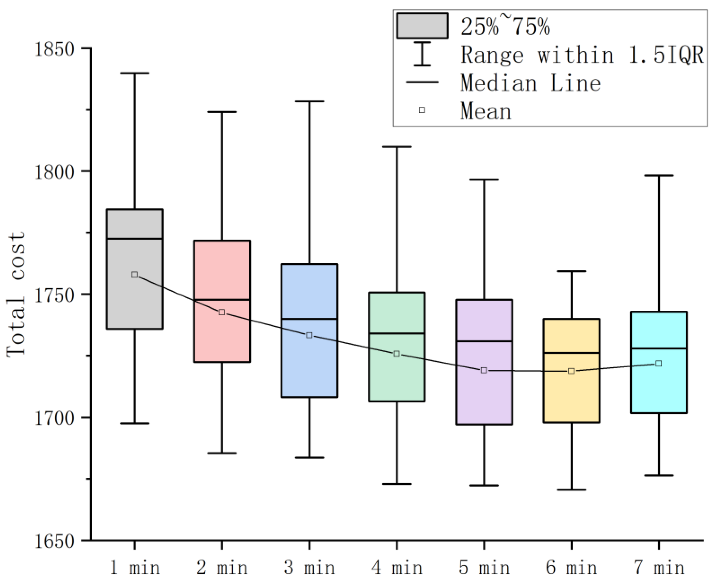
In Table 6, the bold numbers represent the minimum objective function values with different pooling time for each instance. Based on the row of “Average”, it is observed that the minimum value is obtained when the pooling time is 6 min. It can be more intuitively seen from Figure 8 that the objective value of each instance demonstrates a trend of first descending and then ascending slowly with respect to the pooling time. From the “8 min” column, it can be seen that when the pooling time is large, there may be a situation where no feasible solution can be found. Therefore, we did not include the data from the “8 min” column in Figure 8. In addition, when the pooling time is 5 min or 6 min, the objective values are very close. Most of the minimum values are obtained when the pooling time is set as 5 min or 6 min. Therefore, it is believed that the best pooling time should be between 5 min and 6 min. In particular, instances 4, 13, 14, and 16 are almost in line with this trend, showing few irregularities. In addition, instance 8 is also basically in line with the trend of falling first and then rising, but the minimum value is obtained when pooling time is 4 min.

To interpret the observed trend, it is assumed that the oracle exists, and the order details are known within 60 min in advance. Then, the global optimal solution can be obtained for the 60 min online scheduling. However, in reality, only the information of a single round can be realized every time, hence only the optimal scheduling for this round can be made. For example, if the pooling time is 5 min, then 60 min will be divided into 12 rounds. We can derive the optimal solution for each round, but for the 60 min as a whole, only 12 local optimal solutions are achieved. If the pooling time is shorter, then each round is a smaller segment relative to the whole, that is, the less information we know in each round, the worse the decision of each round is made for the whole. This explains why the value of the total objective function decreases with the increase of the pooling time at the beginning. Based on the experimental results, we know that the descending trend is not kept. When the pooling time increases to a certain value, the total objective function value will rise again. It is conjectured that the ascending trend is due to the time window of each order. When the pooling time becomes larger, it will cause the collected orders to be waiting longer, which means that the actual remaining time window of the order could be rather narrow when these orders enter the scheduling stage. In the meantime, it also leads to fewer valets available for these orders and makes scheduling difficult, which ultimately gives rise to the final objective function value. For example, suppose that the original time window width of each order is 15 min and the pooling time is 10 min. Imagine that there is an order, and its order release time is at 11 min, that is, the time window of this order is (11, 26). Then, the order will be pooled in the (10, 20) round. When pooling completes and scheduling starts, the widest time window of this order is only (20, 26), which makes the scheduling rather difficult for this order. In particular, an extreme situation is considered where the pooling time is greater than the original time window width of the order, which causes the problem to be infeasible. This also explains why the total objective function value starts to increase when the pooling time exceeds a certain value. Hence, in combination with the impact of the length of the pooling time on the scheduling described above, it offers a possible explanation for the changing pattern of the total objective function value with respect to the length of pooling time.

6.3. Impact of the Scheduling Time

In this section, the impact of scheduling time on the OVDP is investigated. As it is known, scheduling time is also a very important parameter for the valet driving platform. The experiment setting is similar to that in Section 6.2, except the length of the scheduling time is adjusted here. The number of valets is set as 100, the number of orders is set to be 300, and the pooling time is supposed to be 5 min. We then test how the total objective function value changes over various scheduling times. A total of 20 instances are generated and tested. For each instance, we only change the value of the scheduling time, keeping other parameters unchanged. The experimental results are shown in

Table 7. The impact of scheduling time on OVDP.

	Scheduling Time
Instance	10 s	20 s	40 s	60 s	3 min	5 min
ins-1	1719.6	1720.5	1720.3	1725.9	1730.5	1738.3 *
ins-2	——	1730.0	1728.2	1728.8	1737.6	1760.4 *
ins-3	——	1750.1	1746.2	1747.2	1761.0	1769.6 *
ins-4	——	1743.6	1747.4	1748.3	1758.0	1777.7 *
ins-5	1791.9	1790.4	1799.0	1803.0	1811.8	1818.4 *
ins-6	——	1749.6	1748.6	1753.1	1771.7	1777.1 *
ins-7	——	1771.7	1771.6	1771.6	1780.0	1794.0 *
ins-8	1743.3	1743.3	1741.7	1740.1	1746.4	1762.0 *
ins-9	1811.4	1811.4	1800.9	1802.7	1814.8	1849.1 *
ins-10	1819.3	1819.3	1815.6	1815.6	1983.5	1991.0 *
Average	——	1771.6	1770.5	1772.4	1832.1	——

and Figure 9.

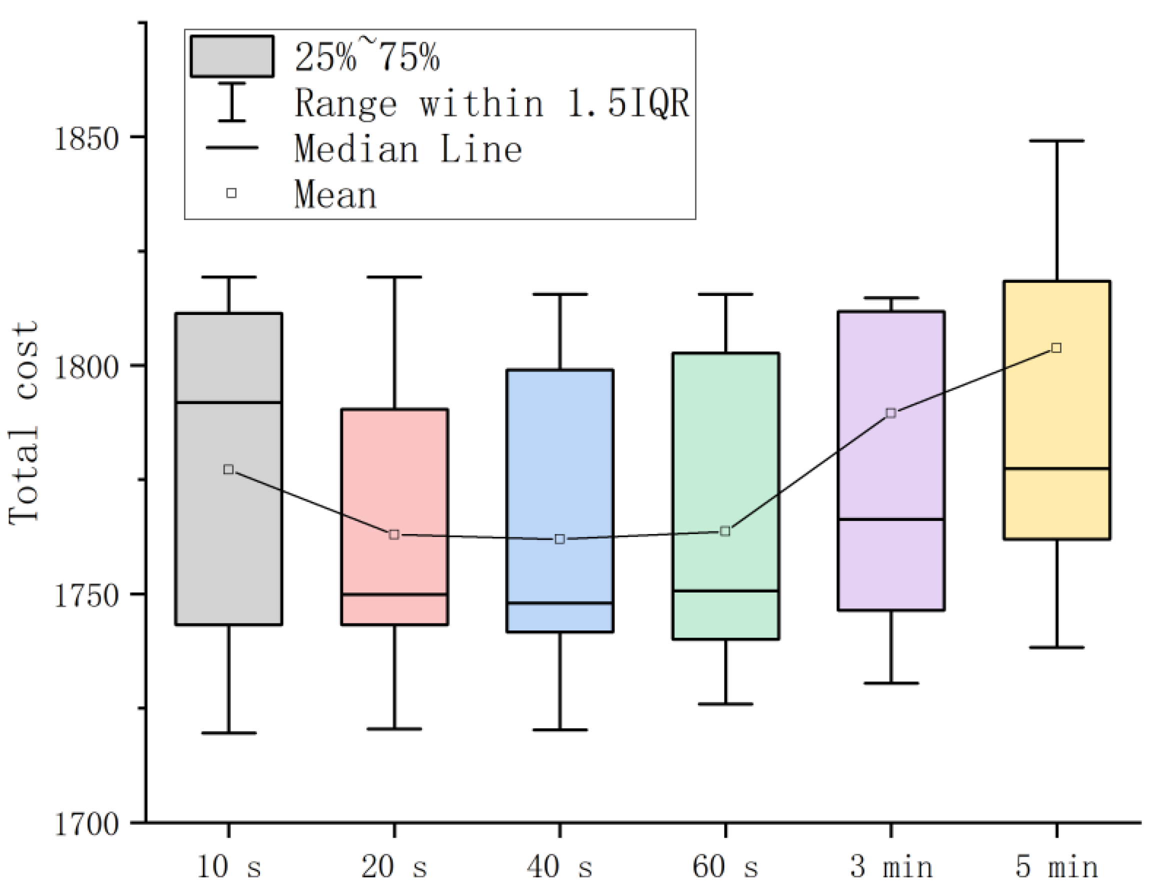
In Table 7, the numbers in bold face and the numbers marked with a star represent the minimum and maximum total objective function values obtained for each instance, respectively. For the column of “10 s”, because the scheduling time is set to be small, it is observed that no feasible solution can be found. However, as the scheduling time increases, as is shown in the column of “20 s”, it is discovered that at least one feasible solution can be obtained for each instance. Based on the bold-face numbers, it is observed that the minimum total objective value of each instance mainly occurs when the scheduling time is 40 s. The maximum total objective value of each instance occurs when the scheduling time is 5 min. From Figure 9, it can be clearly observed that the value of the overall objective initially decreases and then increases.

To shed light on the above trend, a possible explanation is provided. On the one hand, when the scheduling time is relatively small, for some instances, it will be difficult to obtain feasible solutions. For longer periods of time, a feasible solution could be obtained, but it is still not optimal. This is why increasing the scheduling time at the beginning will reduce the total objective value. On the other hand, during the scheduling, some valets may experience idleness and wait for the platform to assign new orders. For such a reason, the longer the scheduling time, the longer the waiting will be for the idle valets. In addtion, longer scheduling time also makes the overall efficiency of valets lower, which naturally leads to the increase of the objective value. Additionally, the longer scheduling time further narrows down the remaining time window when assigning the orders. For example, when the scheduling time is longer than the width of the original time window of the order, the completion of the scheduling surely exceeds the time window. Therefore, when the scheduling time increases after reaching the minimum objective value, an ascending trend is expected. Eventually, no feasible solution can be obtained when not enough time is left for the scheduling process. In addition, the scheduling time should be smaller than the pooling time. Otherwise, when the next round of pooling is over and the scheduling is about to be performed, the scheduling result of the previous round will not be known. Therefore, for the valet driving platform, the scheduling time cannot be set too short or too long; the best scheduling time should be somewhere in the middle, preferably 40 s as a rule-of-thumb.

7. Conclusions

This study focuses on the online valet driving problem with pooling time. The problem is to schedule a cohort of valets to serve the driving orders, which are dynamically released on the platform, with an objective to minimize the total operational cost. To reach the customer site, the valet usually rides on a foldable e-bike, the power level of which is considered as a constraint to fully address the OVDP. Directly handling the OVDP would be difficult and time consuming, thus we decompose the online model into a series of static subproblems. The planning horizon is divided into several segments, each of which is composed of pooling and scheduling stages. To analyze the static valet driving problem, an arc-flow programming model is established, which is then reformulated into a set partitioning form. An exact algorithm based on branch-and-price is designed to obtain the optimal solution to the static subproblem. In order to accelerate the computation process, a label setting algorithm as well as an artificial column technique are employed. In the numerical analysis, the effectiveness of the proposed algorithm is verified. The proposed algorithm outperforms Cplex in terms of computational efficiency and quality of solutions. As a byproduct, the impacts of pooling time and scheduling time on the online valet driving problem are investigated. It is discovered that the best pooling time is around 5 min, and the most suitable scheduling time is approximately 40 s for most of the instances.

The findings of the present paper reveal that the proposed new scheduling strategy ensures efficient crew scheduling while taking into account the real-time requirement of orders. This algorithm can be applied to current valet driving platforms, and it brings social welfare to valet driving platforms, valet drivers, and ordinary consumers. The most direct benefit is that it can help such platforms better dispatch their valet drivers, thereby reducing the cost of providing valet driving service and allowing valet drivers to complete more orders in a single shift. In addition, the reduction in the cost of valet driving services will also lead to more customers choosing valet driving instead of risky drunk driving, thereby reducing the occurrence of DUI related accidents. With the development of valet driving services, more gig job opportunities will be created and provide additional benefits to society.

In the future, more complex situations of the OVDP should be considered, such as order cancellation. In particular, the valet driving platform selectively abandons a portion of orders when there are insufficient valet drivers. In terms of solving speed acceleration, more advanced algorithm designs in the B&P could be explored, such as bidirectional labeling algorithms and incorporating various valid inequalities.