2. Mathematical Preliminaries
Let
G be a graph on
n vertices. The
k-th Stirling number of the first kind of
G, denoted by
, is the number of partitions of
G into exactly
k disjoint cycles, where a single vertex is a 1-cycle, an edge is a 2-cycle, and cycles of order three or higher have two orientations. The graphical factorial of
G, denoted by
, is the total number of such decompositions without any restrictions on the number of cycles involved, i.e.,
. For results regarding the Stirling numbers of the first kind and graphical factorials for families including paths, cycles, complete bipartite graphs, and fans, among others, see articles by Barghi [
5] and DeFord [
6]. These results were initially motivated by a combinatorial model of seating rearrangements presented by Honsberger [
7] and further analyzed by Kennedy and Cooper [
8] and Otake, Kennedy, and Cooper [
9].
We showed [
1] that for any tree
T on
n vertices and any integer
,
where
and
are the star and path of order
n. Consequently, we have
We now define global closeness and between centralities. Let
G be a connected graph. For a vertex
v, closeness is defined as
where
is the distance between
u and
v. The global closeness centrality, which is a Freeman centrality measure [
10,
11], can be defined as
where
,
is a vertex in
G such that
, and
H is the maximum value the nominator of
realizes for all connected graphs of order
n.
For a vertex
v in a graph
G, the betweenness centrality is defined as
where
is the number of shortest paths from
u to
w and
are such paths that go through
v. We divide by
to normalize this centrality measure. The global betweenness centrality, which is a Freeman centralization [
10,
11], is defined as
where
,
is a vertex in
G such that
, and
H is the maximum value the nominator of
realizes for all connected graphs of order
n. In the case of
it does not matter whether we use a normalized or nonnormalized definition for
.
We showed [
1] that for any tree
T of order
n, where
,
and
For more information on different centrality measures, especially in the context of social networks, see a paper by Borgatti [
12].
We now define distinguishing polynomials for trees. First, we need to define them for rooted unlabeled trees. For a rooted tree
, where
r is the root, the primary subtree is a subtree
S of
such that
S has the same root as
and every leaf of
is either a leaf of
S or is a descendant of a leaf of
S. For a primary subtree
S of
, we define
, where
is the number of leaves of
S that are leaves in
and
is the number of leaves of
S that are internal vertices in
. By convention, the root in a rooted tree is considered an internal vertex even though its degree might be one. The polynomial
, which we call a distinguishing polynomial, is defined as
, where the sum is over all primary trees of
. Liu [
4] shows that
is a complete isomorphism invariant for rooted unlabeled trees.
For an unrooted and unlabeled tree
T, the distinguishing polynomial
is the product of
, where
l is the number of leaves in
T and
is a rooted tree obtained from
T by contracting an edge incident with a leaf and declaring the resulting vertex the root of
. Liu [
4] also shows that
is an isomorphism invariant polynomial for unrooted and unlabeled trees.
One way to define a total ordering on trees of order
n using
is to order them by evaluating
at appropriate values of
x and
y. In this approach, we find
for which
for any unrooted and unlabeled trees
of order
n such that
. We call this method of ordering trees of a fixed order, the evaluation-based total ordering and the two extremes of this total ordering are realized at the path and star of order
n. In this paper, we use this approach to classify trees of order
n by evenly dividing the associated evaluation-based total ordering into two classes and identifying the class containing
and
as “path-like” and “star-like”, respectively. For a more detailed discussion of distinguishing polynomials, see papers by Liu [
4] and Barghi and DeFord [
1].
3. Exact Computations
In this section, we describe algorithms for the exact enumeration of Stirling numbers of the first kind on trees. We note that using the loop-erased random walk algorithm of Wilson [
13], we can generate uniform spanning trees on
n vertices beginning with
. This allows us to empirically estimate the distribution of Stirling numbers of the first kind for these trees as well as the expected distributions of several common metrics studied on graphs. We use these values to inform our parameter selection and classification of trees below. Additionally, as mentioned in
Section 1, trees of a fixed size interpolate between being path-like and star-like with respect to many graph metrics. To sample more efficiently from these extremes, it is possible to implement a weighted version of the cycle basis walk on spanning trees, and the autocorrelation of this model is analyzed in the first section of the Supplementary Information. The Supplementary Information is posted on our corresponding GitHub repository for this paper; for a link to this repository, see our Data Availability Statement.
In addition to uniform trees, it is also possible to efficiently sample uniform cycle covers for bipartite, planar graphs, building on the method of Jerrum and Sinclair [
14,
15] for sampling uniform perfect matchings. This is described in Algorithm 1 below. Next, we observe that while computing the
k-Stirling numbers of the first kind can be computationally intensive, computing the graph factorial, which is the sum of these numbers over
k, can be done with a single matrix determinant for planar graphs using the FKT algorithm described in Section 1.2 and Theorem 1.4 in a book by Jerrum [
16]. This algorithm, introduced in a paper by Kasteleyn [
17], counts the number of perfect matchings in a planar graph by constructing a Pfaffian orientation in polynomial time. This is a simple example of the permanent-determinant method [
18]. By modifying the Pfaffian with polynomial entries we can compute the number of 2-cycles that appear in the cycle cover as the coefficient of
. We provide implementations of these algorithms in our corresponding GitHub repository and present examples in the section below motivating conjectures for uniform trees.
| Algorithm 1: Uniform Cycle Cover |
 |
Theorem 1. Algorithm 2 returns the number of matchings of T across all .
Proof. The permanent adjacency matrix of a tree T counts the cycle covers of T. These correspond to matchings since the only possible cycle lengths are 1 and 2. Let be the adjacency matrix of T. We note that viewing as a biadjacency matrix gives , which is planar since T is outerplanar. Thus, we can apply the FKT algorithm to to obtain a Pfaffian orientation of . This means that the number of perfect matchings in the product can be computed as the square root of this number, which is exactly the number of cycle covers that we were trying to compute. □
| Algorithm 2: Tree Stirling |
Input: A tree T Output: The number of k-matchings of T for all k Construct Orient the adjacency matrix A of G with FKT Multiply the non-diagonal elements of the signed matrix by x Compute Return: |
There is also an algebraic method for computing these values by representing the terms with a symbolic determinant.
Theorem 2. The determinant of returns the number of matchings of T across all as the coefficient of .
Proof. A non-zero term in the determinant of consists of a set of diagonal elements S counted with a weight of positive one and a perfect matching of where each term collects a weight of . The product of these terms is then equal to where k is the number of edges of T that occur in the matching. Summing up over all permutations of the nodes in the determinant gives that the coefficient of is the desired number of k-matchings. We note that a similar argument shows that the determinant matrix of with the upper-triangular portion negative also returns the same values as coefficients and the determinant of the unsigned matrix returns the values with signs according to the parity of k. □
Although the above results show that the problem of enumerating the number of cycle covers of a given size can be completed in polynomial time in the number of nodes in the tree, actually generating the cycle covers themselves is a more difficult problem. The reason that computing the complete list of cycle covers for graphs is computationally taxing is that even for trees and forests we need to rely on a modified version of the classic deletion-contraction algorithm described in Chapter 2 of [
19] and Chapter 1 of [
20], which we call the deletion–inclusion algorithm. In the deletion–inclusion algorithm, for an edge
e in a forest
F, we either delete
e or we contract
e and remove all the other edges incident with the endpoints of
e. Since this is a binary branching algorithm, we continue with this process in each branch until there are no edges left to remove in the said branch. If the order of the empty graph at the end of a branch is
k, it contributes to
. The advantage of the deletion–inclusion algorithm to the uniform cycle cover is that it produces the set of all cycle covers of
F while the running time of the two algorithms, at least for small enough trees, is comparable.
| Algorithm 3: Deletion-Inclusion Step |
Input: A forest F Output: A contracted edge E and two sub-forests , and with Select: A uniformly random edge Compute: Remove and Contract: Contract Return: |
| Algorithm 4: Deletion-Inclusion |
 |
| Algorithm 5: Generate Cycle Covers |
 |
We note that this generation process can be carried out in a polynomial time for fixed k and n by evaluating the many one-cycles for perfect matchings, which suggests that we should be mindful of letting n and k grow simultaneously, particularly when k is close to .
To provide a complete implementation of the algorithms described in this section, we also included the
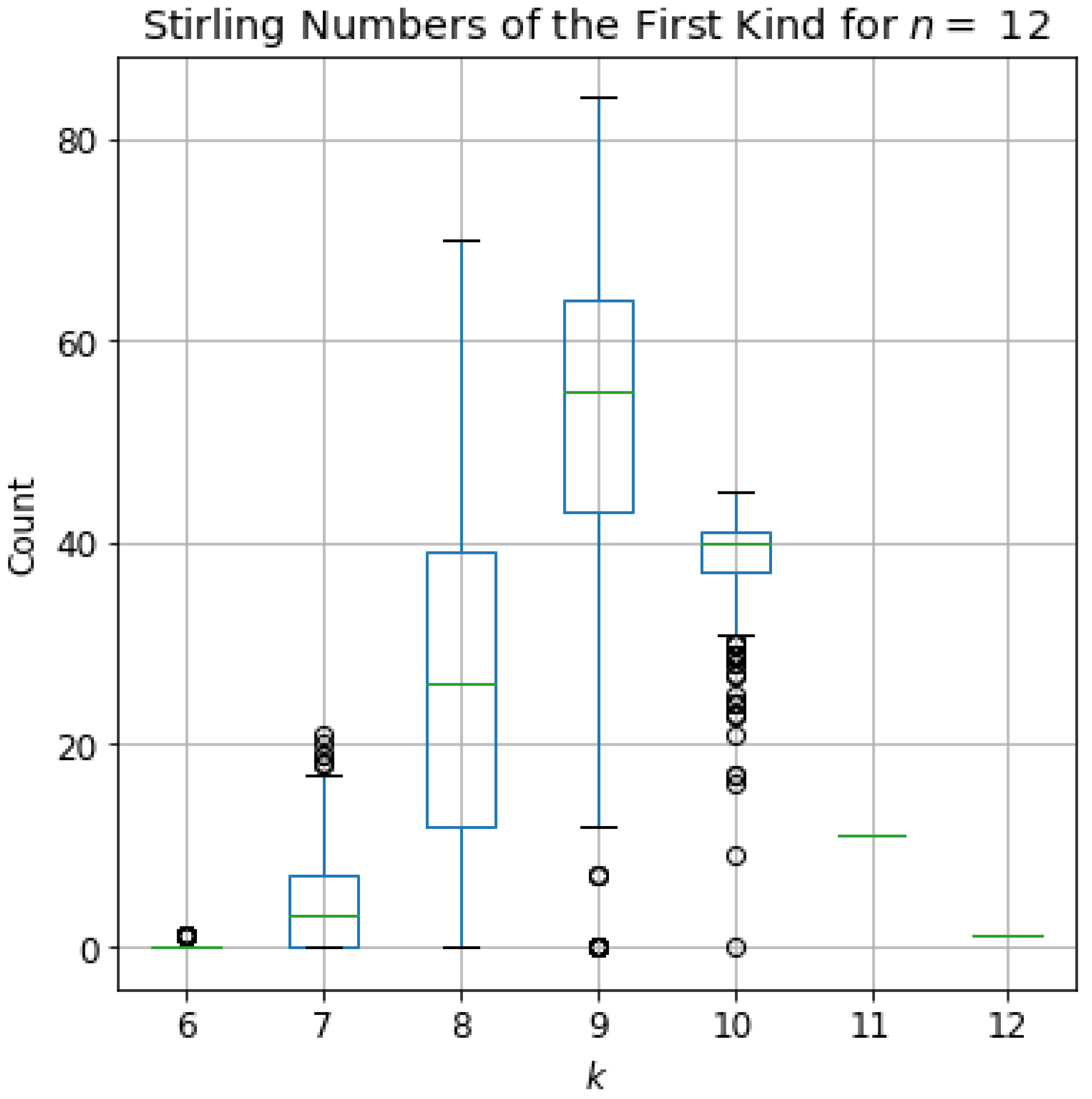
Python scripts in our GitHub repository. In
Figure 1, we use these methods to compute all
k Stirling numbers across all isomorphism classes of trees on
nodes. These are representative of the values that we use in
Section 5 as inputs to the statistical learning methods.
4. Probabilistic Approach
Our next approach for computing Stirling numbers of the first kind is probabilistic, applying techniques from matrix algebra.
Let
F be a forest and let
V and
E be its vertex and edge set, respectively, with
c connected components. Let us assume that
; hence,
. Suppose
is a partition of
F into
k cycles. For
, denote the set of incident edges with
v by
. For every
, where
, define
as follows:
With this definition in mind,
where these conditions are as follows:
If we denoted the set of vertices in 1-cycles and 2-cycles by A and B, respectively, then . Please note that , and . It follows that . As a result, .
Let A be the incidence matrix for a forest F and the column vector , then is a -column vector with exactly many 1’s and many 0’s. Reversing the previous discussion gives the following result that we can use to develop an approximation algorithm.
Lemma 1. For any -column vector with many 1’s and many 0’s, the probability that the linear equation has a -solution is:where F is the forest with incidence matrix . The previous result suggests an algorithm for estimating by sampling uniformly from the set of binary vectors with exactly many 1’s, and determining whether the solution to has binary entries.
For , let be a -column vector with many 1’s and many 0’s random entries and let . Solving the equation , where is a matrix of unknowns column vectors . The time complexity of applying Gaussian elimination to the augmented matrix is . Using back-substitution to find a solution for is and checking whether this solution consists of only 0s and 1s require operations. With m random vectors , we need operations. Therefore, the overall time complexity of checking which random column vectors yield an allowable solution requires operations, assuming c is fixed.
This naive approach requires fully solving the associated linear system and checking whether the resulting solution vectors are binary. We can circumvent this computational hurdle by instead interpreting the system as a collection of Diophantine equations, motivated by interpreting the product as occurring over the edges of the tree, rather than the vertices.
Note that
It follows that
and
Now define
as
for every
. It follows that
Additionally, the restrictions on
’s translate to the following restrictions for
:
If for some , then .
If for some , then .
It follows that
and
, and
In general, without any restrictions, the number of
-solutions to the Diophantine equation
is
. This implies the following result that allows for a more efficient randomized method.
Lemma 2. Let be a binary vector indexed by the edges of F. Then the probability that the positive entries of Y induce a partition of F into k cycles and hence correspond to edges that are not 2-cycles in is As with the previous approximation result, Lemma 2 suggests an algorithm for estimating by sampling uniformly from the set of binary vectors indexed by the edges of F, and determining whether they induced a partition with the proper number of cycles.
If
is the column vector whose entries are 1’s and
is the incidence matrix of
F, then
is column vector containing the degree sequence of
F. On the other hand, if
satisfies the conditions in (
1), then
should consist of
many 1’s. If we have
m many
-column vectors
with random entries consisting of
many 1’s, then the time complexity to check whether each one satisfies the conditions in (
1) is
and the overall time complexity is
, which may be more efficient than our earlier approach.
For an implementation of this approach in
Python, on our GitHub repository, see the
Jupyter notebook
TreeLearning-Testing_Probabilistic_Approach.ipynb. In this notebook, a random tree
T is generated, so the number of components
c is one. The code generates
m trials. At each trial, a
-column vector with random entries is generated and a trial is considered a “success” if the condition that it contains exactly
many 1’s is met. We use a Bernoulli random variable to represent the outcome of each trial. In other words, we denote the random variable representing the
ith trial by
where
p is the probability of “success”. The main objective is to estimate
via simulation. Let
. Since
, we calculate
in the code to see how well this probabilistic approach performs.
Results
To make our code reproducible, we are using a random seed. The results for
n between 7 and 15 and
,000 is included in
Table 1. For each
n, a random tree
T of that order is generated and
is estimated for
.
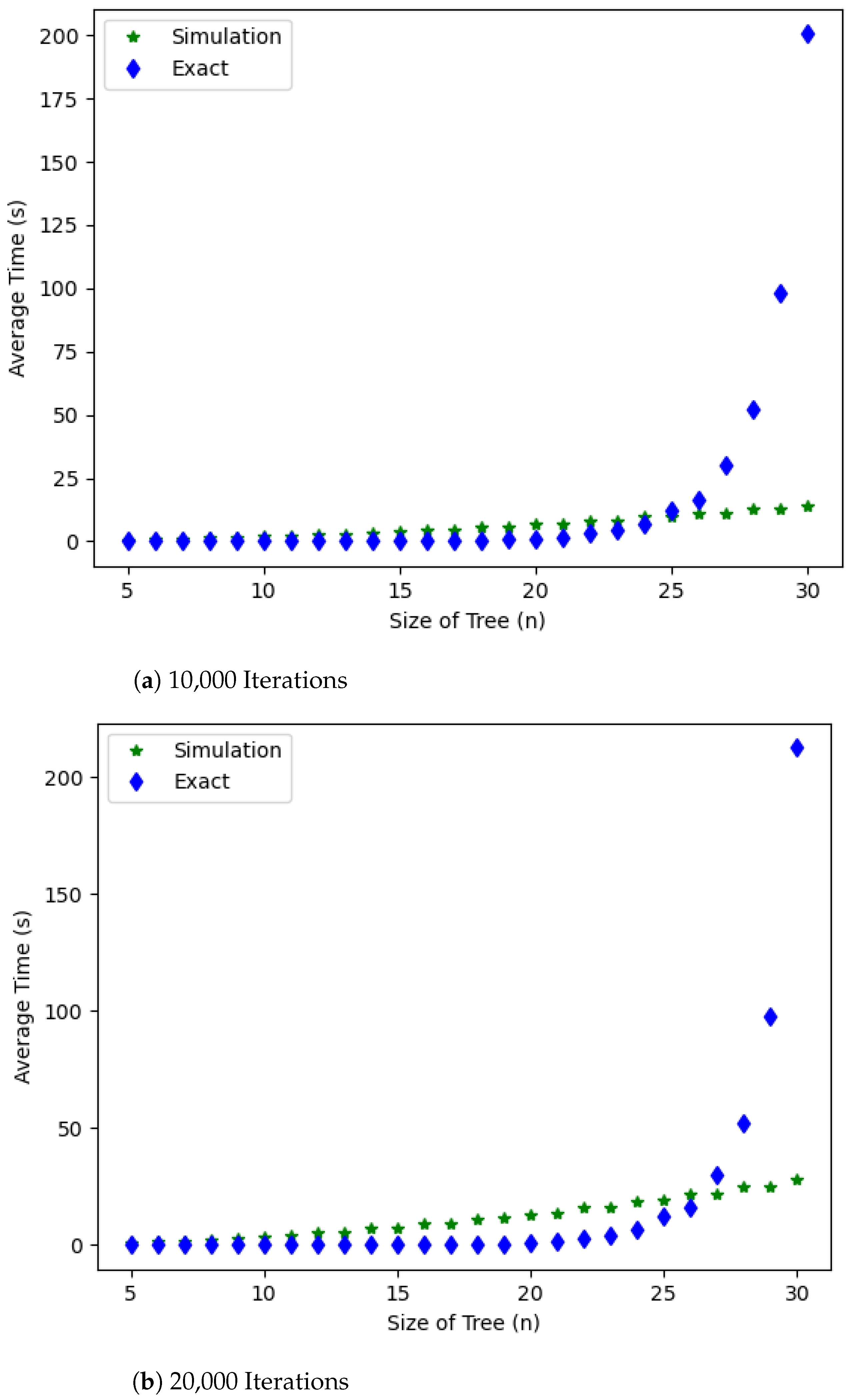
One natural question is how the probabilistic approach performs compared to the exact computation of
. In
Figure 2, the average running times for the probabilistic approach for estimating and the exact method for computing
for
, for
, and a random tree
T of order
n, are visualized. As we see in
Figure 2, the average running times for using the probabilistic approach grows linearly while the exact computation grows exponentially, and the average running times using exact computation take over those of the probabilistic approach when
for 10,000 iterations and
for 20,000 iterations. The code to reproduce these plots is in the following
Python script:
probabilistic_approach–average_running_times.py. Note that the running time for this
Python script is long.
The Python script probabilistic_approach–uniform_sampling.py on the GitHub page computes the difference between the exact value of the k-th Stirling number and its approximation using the probabilistic approach discussed above for 100 trees of order n uniformly sampled using the Wilson algorithm for and . This Python script returns separate .csv files for each n. On the other hand, the Python script analysis–probabilistic_approach–uniform_sampling.py computes the mean, standard deviation, and skewness of these differences for each n and each k. As shown in the table in the second section of the Supplementary Information, the mean of these differences stay relatively close to zero and, with the exception of a few extreme values of k, the skewness of these differences also stay relatively close to zero, indicating symmetric distributions. Since, in this experiment, we do not scale m along with n and we take uniform samples of size 100 for each value of n from the space of tree of order n, the standard deviations increase as n increases, as expected.
5. Statistical Learning and Enumerative Metrics on Trees
Many interactions between combinatorial analysis and modern machine and statistical learning techniques have focused on the field of combinatorial optimization [
21,
22,
23]. These analyses have both applied learning techniques to generating heuristics or approximate solutions to difficult combinatorial problems [
24,
25,
26,
27], as well as motivating interesting new areas of combinatorial research [
28]. Another recent area of interest is Graph Neural Networks [
29,
30] which use graph structures to better represent features in modern datasets. Other techniques that have motivated work between these fields include determinantal point processes [
31,
32,
33] and submodular functions [
34,
35,
36], which have the same property of providing solutions to difficult problems and providing interesting new avenues of study. In this paper, we do not consider an optimization approach but rather use the combinatorial structure reflected in the enumeration of Stirling numbers and other network statistics as input and training data for classification and regression.
As we discussed earlier, the
k-th Stirling number of the first kind (for fixed
k), global closeness centrality, and global betweenness centrality for trees exhibit a similar property in that their values varies between two extremes which are realized at paths and stars. In other words, for any tree
T on
n vertices and any integer
,
and
Based on these observations, we use statistical learning tools and use Stirling numbers of the first kind for trees as predictors to make predictions about members of random sets of trees, both in the training and testing stages. It is assumed that trees in both the training and testing sets have a fixed number of vertices and there is the same number of trees in both training and testing sets. Moreover, we use both classification and regression algorithms to address this problem.
We will use three separate datasets while using statistical learning methods. The first dataset consists of all non-isomorphic trees of order 12, of which there are 551, using the networkx.nonisomorphic_trees function. First, we classify these trees by evenly dividing the associated evaluation-based total ordering into two classes and identifying the class containing and as “path-like” and “star-like”, respectively. We then evenly split the trees into a train and test set at random. For reproducibility purposes, we use a random seed in our code.
In the second dataset, using a random seed, we generate 500 non-isomorphic trees of order 18 using the networkx.nonisomorphic_trees function. Again, we classify them as “path-like” and “star-like” by evenly dividing the associated evaluation-based total ordering. Note that a tree might be misclassified as opposed to its class if we used the complete list of non-isomorphic trees of order 18, but we expect the number of such misclassifications to be low. Again, we evenly divide these 500 trees into a train and test set at random. Because we can generate a separate test set, we will not be using cross-validation and out-of-bag error estimation in our code. Lastly, in the third dataset, we generate 500 trees of order 18 sampled uniformly from the space of such trees.
We use the following classifiers from scikit-learn library [
37] in
Python:
For DecisionTreeClassifier, ExtraTreeClassifier, RandomForestClassifier, and ExtraTreesClassifier, we used both Gini and entropy criteria, which are measures of node impurity when fitting these models. We also used Minimal Cost-Complexity Pruning in these models. And to compare methods based on their performance on train and test sets, we use the following classification metrics: accuracy_score, confusion_matrix, matthews_corrcoef, and classification_report.
To estimate Stirling numbers of the first kind for trees, we will use the following regression models from scikit-learn library [
37]:
LinearRegression
Ridge
Lasso
ElasticNet
PolynomialFeatures (for degree 2 regression)
SGDRegressor (Stochastic Gradient Descent)
DecisionTreeRegressor
ExtraTreeRegressor
RandomForestRegressor
ExtraTreesRegressor
BaggingRegressor
SVR (Support Vector Regression)
To measure how these methods perform on train and test sets, we use the following regression metrics: r2_score, explained_variance_score, and mean_squared_error.
5.1. Results
5.1.1. Classification
The results for tree-based and support vector classification methods with closeness, betweenness, and for as predictors for all non-isomorphic trees of order , for a sample of size 500 of non-isomorphic trees of order generated randomly using networkx.nonisomorphic_trees, and for a sample of size 500 of trees of order sampled uniformly from the space of all such trees using Wilson’s algorithm are in the tables in the Supplementary Information. In this experiment, the response is class, i.e., whether a tree is “star-like” or “path-like”. These results are computed by running the code in the Jupyter notebooks in our GitHub repository. As shown in the tables in the third and fourth sections of the Supplementary Information, tree-based classifiers (decision tree, extra tree, bagging, random forest, and extra trees) individually perform comparably on train and test sets so do support vector classifiers (linear and quadratic SVC). Additionally, across these methods, we also see comparable performances on test sets and train sets, separately, which suggests that trained models generalized nicely to unseen data, regardless of the method used. Here we are considering both accuracy scores and Matthews’ correlation.
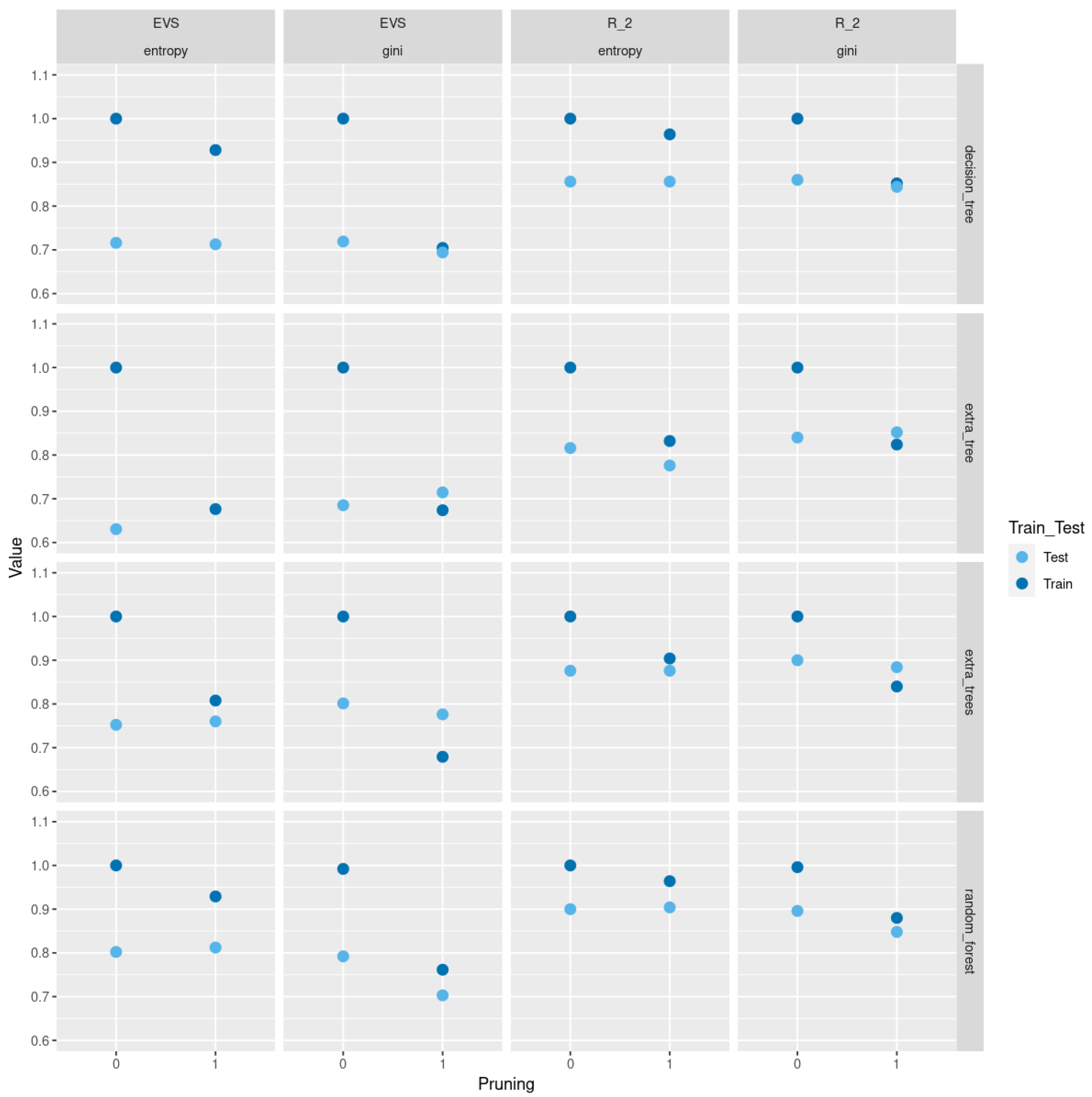
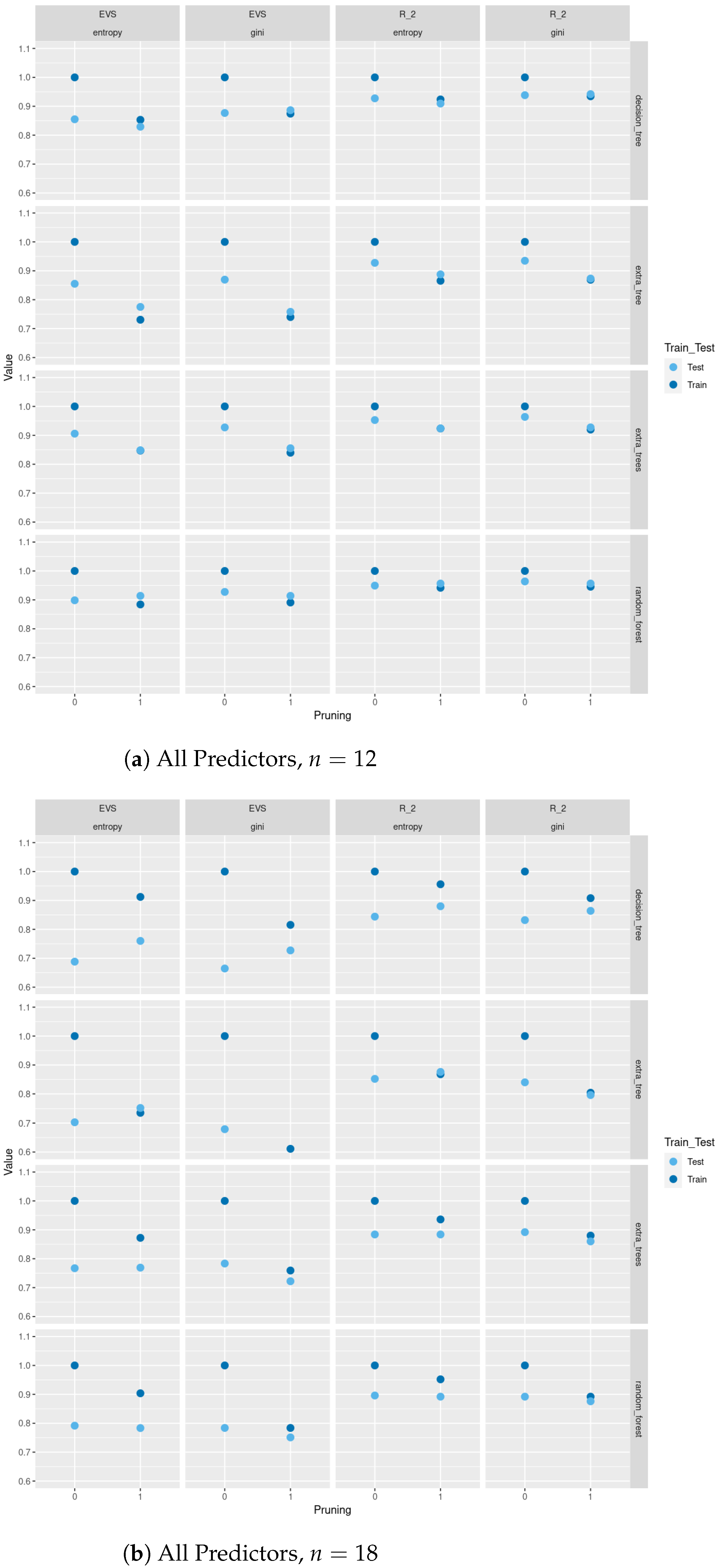
In
Figure 3, we compare between train and test
scores and explained variance scores (EVS) between different tree-based classification methods based on Gini and entropy criteria with and without pruning for a sample of size 500 of trees of order
sampled uniformly from the space of all such trees using Wilson’s algorithm. As we see in
Figure 3, pruning does not lead to a severe decrease in test
scores and EVS and in some methods we see an increase in these scores. Of course, pruning leads to a decrease in train
score and EVS, but the trade-off is that the resulting models are trees with less depth, fewer nodes, and less complexity and the same level of test performance. Moreover, using the two different sampling methods for trees of order
, does not lead to a difference in results. In
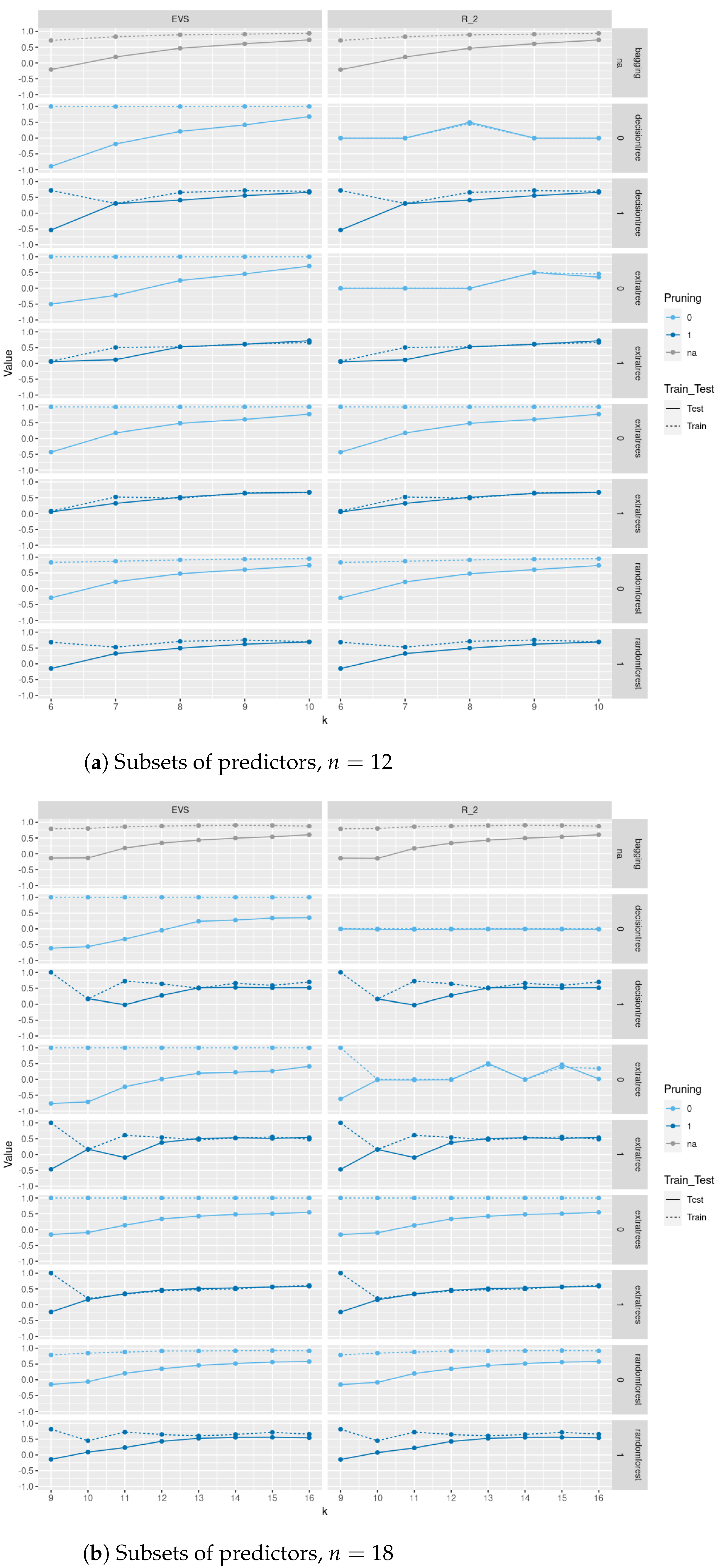
Figure A2 and
Figure A3, we do a similar comparison for all non-isomorphic trees of order
and for a sample of size 500 of non-isomorphic trees of order
generated randomly using
networkx.nonisomorphic_trees.
To compute the results for closeness, betweenness, and Stirling numbers of the first kind for trees as sole predictors, one may run the code in the Jupyter notebooks in our GitHub repository.
5.1.2. Regression
For regression and tree-based regression methods, we use , closeness, betweenness, and class as predictors for all non-isomorphic trees of order , for a sample of size 500 of non-isomorphic trees of order generated randomly using networkx.nonisomorphic_trees, and for a sample of size 500 of trees of order sampled uniformly from the space of all such trees using Wilson’s algorithm, respectively, to predict for . These results are computed by running the code in the Jupyter notebooks in our GitHub repository.
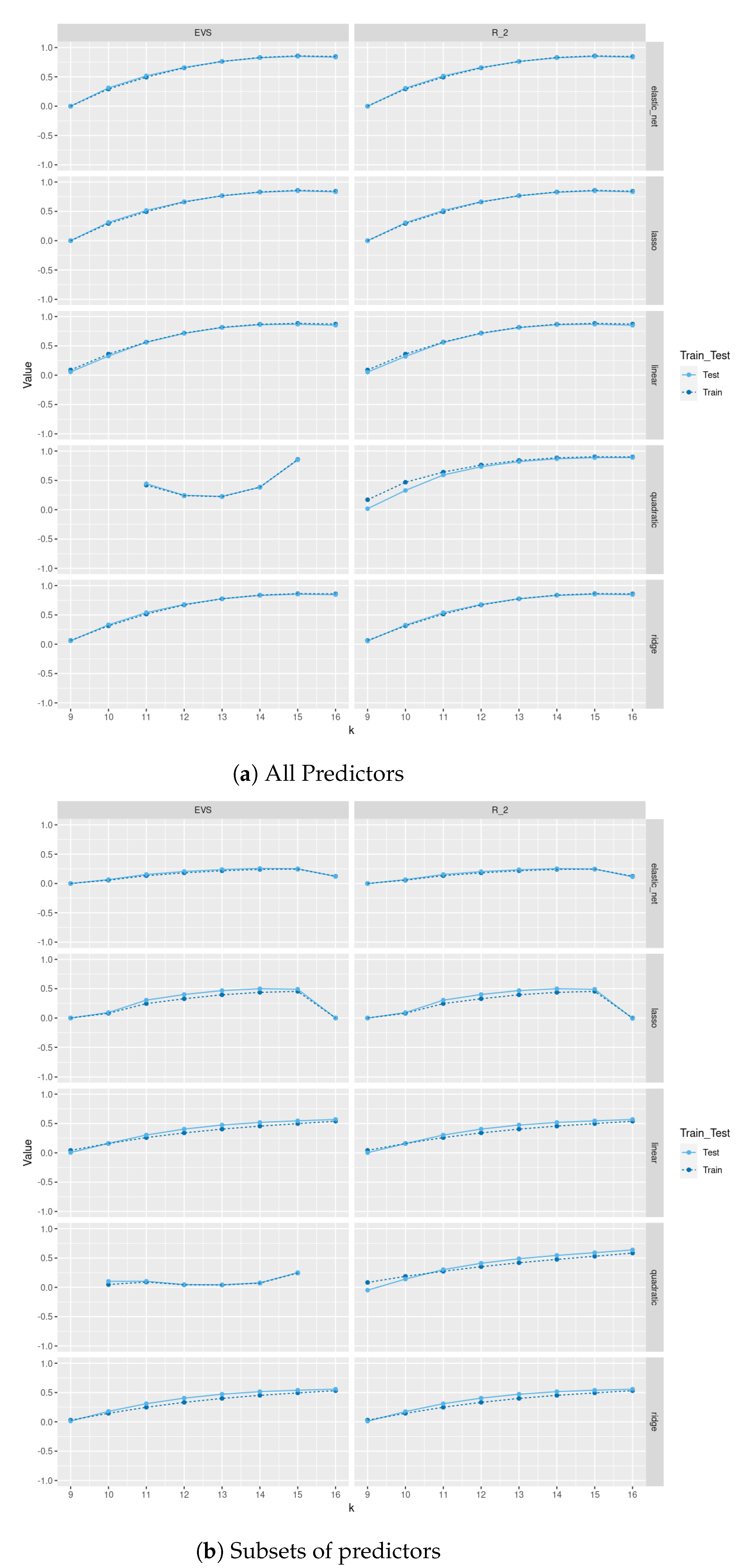
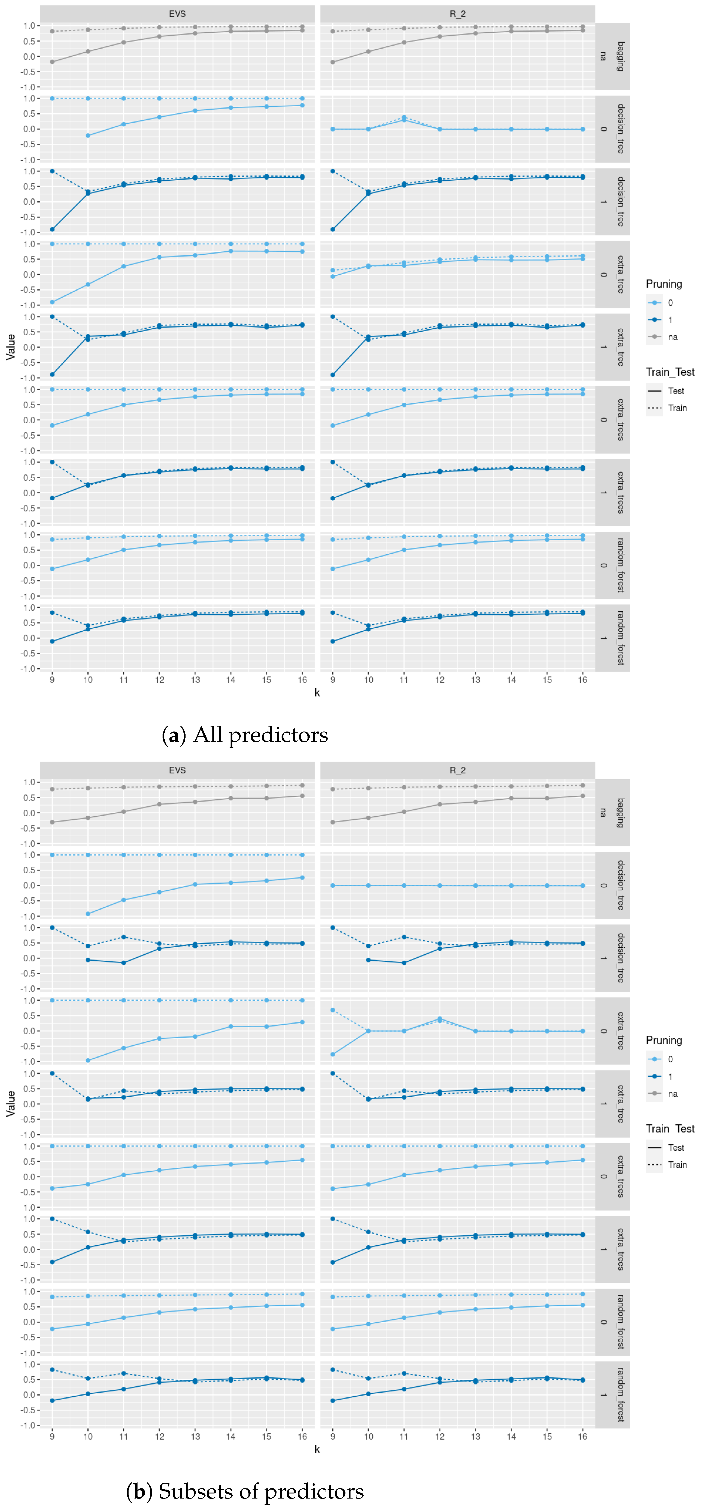
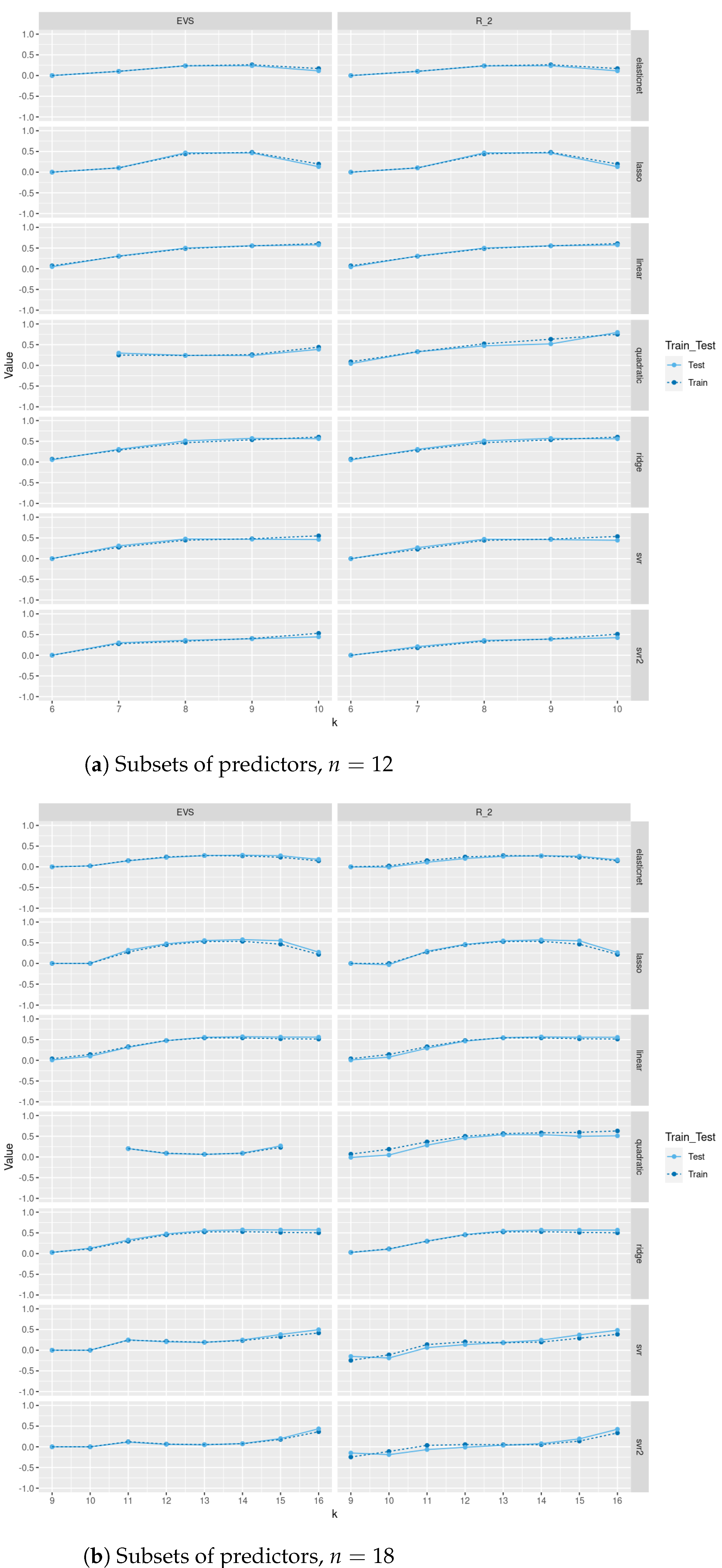
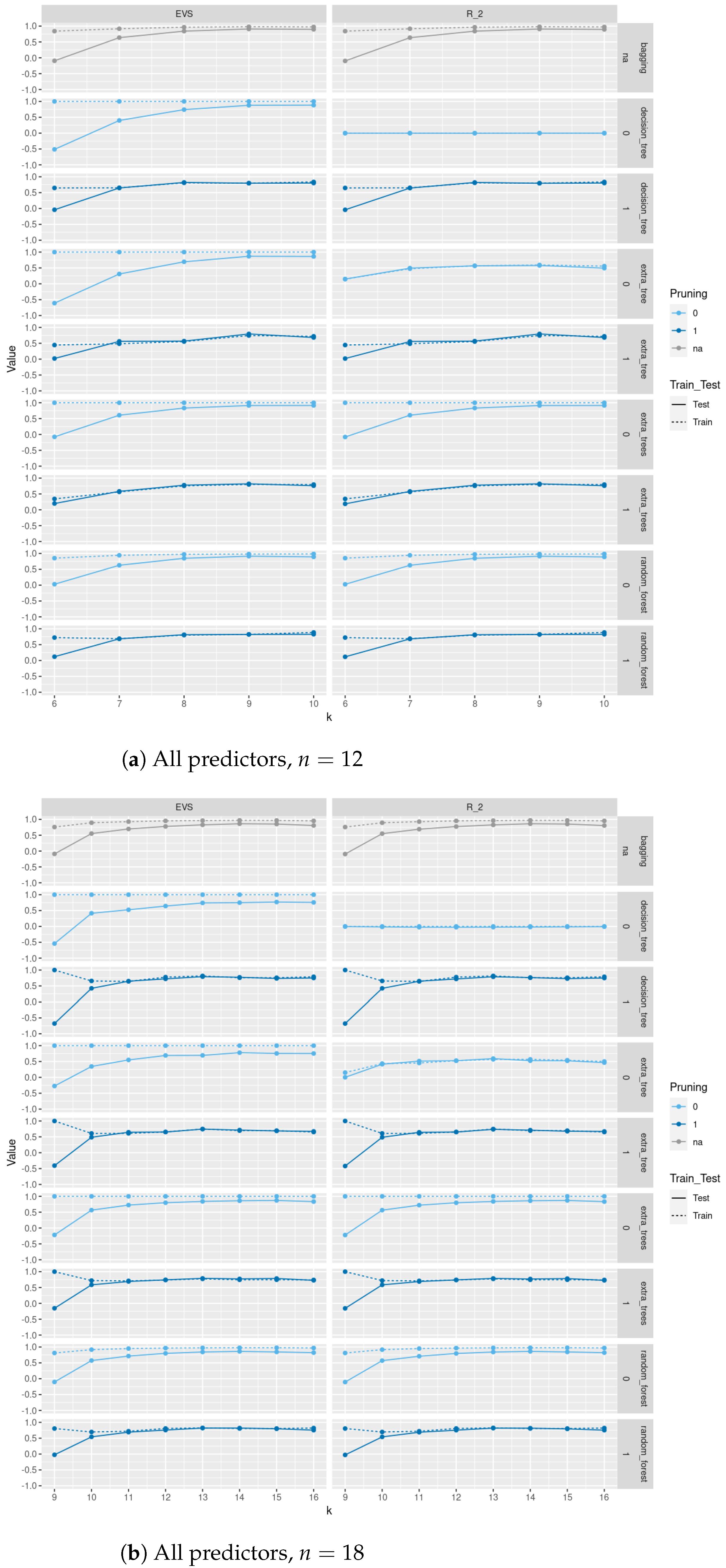
In
Figure 4 and
Figure 5, we compare between train and test
scores and explained variance scores (EVS) between different regression and tree-based regression methods (with and without pruning), respectively, for a sample of size 500 of trees of order
sampled uniformly from the space of all such trees using Wilson’s algorithm. As we see in
Figure 4, pruning does not lead to a severe decrease in test
score and EVS and in some methods an increase in these scores. Of course, pruning leads to a decrease in train
and EVS, but the trade-off is that the resulting models are trees with less depth, fewer nodes, and less complexity and the same level of test performance. Moreover, excluding
as one of the predictors severely affects the performance of these models on train and test sets. Please note that the values in these plots are those between −0.5 and 1; specifically, values less than
are not included. In
Figure A2,
Figure A3,
Figure A4, and
Figure A5, we do a similar comparison for all non-isomorphic trees of order
and for a sample of size 500 of non-isomorphic trees of order
generated randomly using
networkx.nonisomorphic_trees. Using the two different sampling methods for trees of order
, does not lead to a difference in results.
In
Figure 5, we see that pruning leads to an almost zero difference between
score and EVS; for the exact values, see in the tables the fifth through seventh sections of the Supplementary Information. This indicates that the mean of residuals is almost zero. We also see that a difference between
score and EVS only exists in decision tree and extra tree without pruning.
To compute the results for closeness, betweenness, and class together as predictors and for as a response, one may run the code in the Jupyter notebooks in our GitHub repository.


