A Novel Classification Algorithm Based on Multidimensional F¹ Fuzzy Transform and PCA Feature Extraction

Abstract

The bi-dimensional F¹-Transform was applied in image analysis to improve the performances of the F-transform method; however, due to its high computational complexity, the multidimensional F¹-transform cannot be used in data analysis problems, especially in the presence of a large number of features. In this research, we proposed a new classification method based on the multidimensional F¹-Transform in which the Principal Component Analysis technique is applied to reduce the dataset size. We test our method on various well-known classification datasets, showing that it improves the performances of the F-transform classification method and of other well-known classification algorithms; furthermore, the execution times of the F¹-Transform classification method is similar to the ones obtained executing F-transform and other classification algorithms.

1. Introduction

The Fuzzy Transform technique (for short F-transform) [1] is a fuzzy regression method introduced to approximate a continuous function of k variables f(x₁,x₂,…, x_k) defined in the domain [a₁,b₁] × [a₂,b₂] ×…× [a_k,b_k] ⊂ R^k. If this function is known in N points p_j = (p_j1, p_j2,…,p_jk) j = 1,…N, it can be approximated by a weighted average whose weights are constants given by the components of the direct F-transform.

F-transform was applied in many image and data analysis problems. An extensive description of the F-transform-based techniques used in image and data analysis is given in [2].

In [3] a generalization of the F-transform, called high degree F-transform and labelled with F^s-transform (s ≥ 0) was proposed, where the F-transform is given by the zero-degree F⁰-transform. In the F^s-transform, with s > 0, the constant components of the direct F-transform, were replaced by s-degree polynomial components with the aim to capture more information about the original function. The greater the polynomial degree, the finer the approximation of the original function; however, as the polynomial degree increases, the computational complexity of the algorithm that uses the F^S transform increases considerably. In addition, the meeting of the constraint of sufficient data density with respect to fuzzy partitions further requires additional consumption of memory resources and CPU time [2,4].

Some researchers apply the F¹-transform in image analysis, in which only two input variables are used, and the sufficient data density constraint is always met. In [5,6] an algorithm based on the F¹-transform in two variables was applied in an image processing edge detection problem. In [7] a lossy image compression method based on the F¹-transform in two variables is proposed; the authors show that this method improves the decoded image quality obtained using the F-transform image compression [8]. In [9] a hybrid deep neural network in which the F^s-transform is used in image analysis to construct in a preprocessing phase the convolution kernels in the first two layers of the network.

Generally, when the multidimensional F-transform is applied in classification, regression, and prediction problems, as the dimensionality of the data increases, the computational complexity greatly increases; for this reason, the application of high-order F-transforms in data regression or classification has a high computational complexity, in terms of memory and time consumption, especially in the presence of massive multidimensional data [4]. An application of the first-order unidimensional fuzzy transform was proposed in [10] where the unidimensional F¹-transform is applied to seasonal time series weather datasets in a seasonal forecasting model. Comparison tests show that this model improves the forecasting time series performances obtained by applying the F⁰-transform model proposed in [11,12]. In [13] the F¹-transform is applied to remove seasonal components and noise in time series.

Recently, in [14] a new classification algorithm based on the multidimensional F⁰-transform for massive datasets called Multi-dimensional F-transform Classification (for short, MFC), was proposed. In MFC the K-fold cross-validation technique is applied to avoid overfitting in the data; the multidimensional direct F⁰-transform is applied to each fold and a weighted mean of the multi-dimensional inverse F⁰-transform calculated from the direct F⁰-transform components obtained in each fold is used to classify data points. Comparisons with well-known classification algorithms showed that MFC has better classification performances than Naive Bayes [15] and Lazy Bk [16] and is comparable with respect to the ones obtained by using Decision tree J48 [17] and Multilayer Perceptron [18] algorithms. On the other hand, the main drawback of this method is the high computational complexity that is reached when the number of features increases.

In [19] a hybrid fast classification method based on F-transform and Principal Component Analysis (for short, PCA) [20,21,22,23] is proposed. This method is tested to classify images; the results show that it improves the success rate and computation time obtained by applying the F-transform algorithm.

PCA is a well-known dimensionality reduction multivariate statistics technique whose goal is to reduce the number of features of a dataset by losing the least amount of information possible. PCA is one of the most used feature extraction techniques in data analysis. Its strong point is to be able to reduce the dimensionality of the data, while preserving their information content.

In this research, we propose a hybrid classification method applied to massive data including the PCA and the multidimensional F¹-transform techniques. The main goals of the proposed method are:

-

Improve the MFC classification performances; the application of the multidimensional direct and inverse F1-transform allows to increase the accuracy and precision of the classifier with respect to the use of the multidimensional F-transform.

-

Significantly reduce the time and memory consumption executing the PCA feature extraction algorithm in the preprocessing phase to reduce the dimensionality of the data.

In Section 2, the concepts of multidimensional direct and invers F¹-transform are introduced and the PCA algorithm is synthetized. Section 3 is focused on the analysis of the architecture and functional characteristics of our classification method based on the multidimensional F1-transform. The results of experimental tests are discussed in Section 4. Finally, in Section 5 the conclusions and future perspectives are included.

2. Preliminaries

2.1. Principal Component Analysis

Data dimensionality reduction techniques are divided into feature selection and feature extraction techniques. Feature selection techniques, such as random forest or grid search algorithms, select a subset of the original features in order to reduce the complexity and computational efficiency of the model. Conversely, feature extraction techniques extract information from the original features set and create a new features subspace. While feature selection techniques aim to select the most significant features, discarding the less significant ones from the set of original features, feature extraction techniques construct a new reduced set of features, starting from the existing ones, able to synthesize most of the information contained in the original set of features.

The use of feature selection techniques is preferable when the explainability of the model and the semantic meaning of the features are required; feature extraction techniques are used to reduce the model complexity, improving its predictive performance.

PCA is one of the most used feature extraction techniques in data analysis. Its strong point is to be able to reduce the dimensionality of the data, while preserving their information content.

Let D be the original dataset with s features X₁, …, X_s and N instances. The ith instance is characterized by a vector (x_i1, x_i2,…, x_is)^T where x_ij is the value of the ith instance in correspondence to the jth feature.

Let m_j be the mean value of the jth feature, given by:

$${\mathrm{m}}_{\mathrm{j}}=\frac{1}{\mathrm{N}}{{\displaystyle \sum }}_{\mathrm{i}=1}^{\mathrm{N}}\hspace{1em}{\mathrm{x}}_{\mathrm{ij}} \mathrm{j}=1,\dots ,\mathrm{s}$$

(1)

and st_j the standard deviation is given by:

$${\mathrm{st}}_{\mathrm{j}}=\sqrt{\frac{1}{\mathrm{N}}{{\displaystyle \sum }}_{\mathrm{i}=1}^{\mathrm{N}}{\left({ \mathrm{z}}_{\mathrm{ij}}-{\mathrm{m}}_{\mathrm{j}}\right)}^2}\hspace{1em}\mathrm{j}=1,\dots ,\mathrm{s}$$

(2)

To remember this definition, we can break it down into eight steps:

1.

The aim of this phase is to standardize the range of the initial variables so that each one of them contributes equally to the analysis. For each instance x_ij, its normalized value is computed, given by:

$${\mathrm{z}}_{\mathrm{ij}}=\frac{{ \mathrm{x}}_{\mathrm{ij}}-{\mathrm{m}}_{\mathrm{j}}}{{\mathrm{s}}_{\mathrm{j}}}\hspace{1em}\mathrm{i}=1,\dots ,\mathrm{N}\hspace{1em}\mathrm{j}=1,\dots ,\mathrm{s}$$

(3)

2.

The relationships among features are analyzed by computing the symmetric covariance matrix C = Z^TZ, where Z^T is the transpose of the normalized matrix Z. The components of C are given by

$${\mathrm{C}}_{\mathrm{jk}}=\frac{1}{\mathrm{N}-1}{{\displaystyle \sum }}_{\mathrm{i}=1}^{\mathrm{N}}{\mathrm{z}}_{\mathrm{ji}}·{\mathrm{z}}_{\mathrm{ik}}\hspace{1em}\mathrm{j}, \mathrm{k}=1,\dots ,\mathrm{s}$$

(4)

3.

In this phase, the s eigenvalues and the s eigenvectors of the covariance matrix are extracted. The eigendecomposition of C is where we decompose C into VDV⁻¹, where V is the matrix of eigenvectors and D is a diagonal matrix in which the diagonal components are the eigenvalues λ_i i =1,…,s and the other elements are equal to 0.

4.

The eigenvalues on the diagonal of D will be associated with the corresponding column in P—that is, the first element of D is λ₁ and the corresponding eigenvector is the first column of P. This holds for all elements in D and their corresponding eigenvectors in P. We will always be able to calculate PDP⁻¹ in this fashion.

5.

In this phase the s eigenvalues are sorted in descending order; in the same way the corresponding eigenvectors in the matrix V are ordered, obtaining the matrix V′, whose columns correspond to the ordered eigenvectors.

6.

The normalized data matrix Z is transformed in the matrix of the principal components Z′ multiplying Z by the ordered matrix of the eigenvectors V′: Z′ = ZV′.

7.

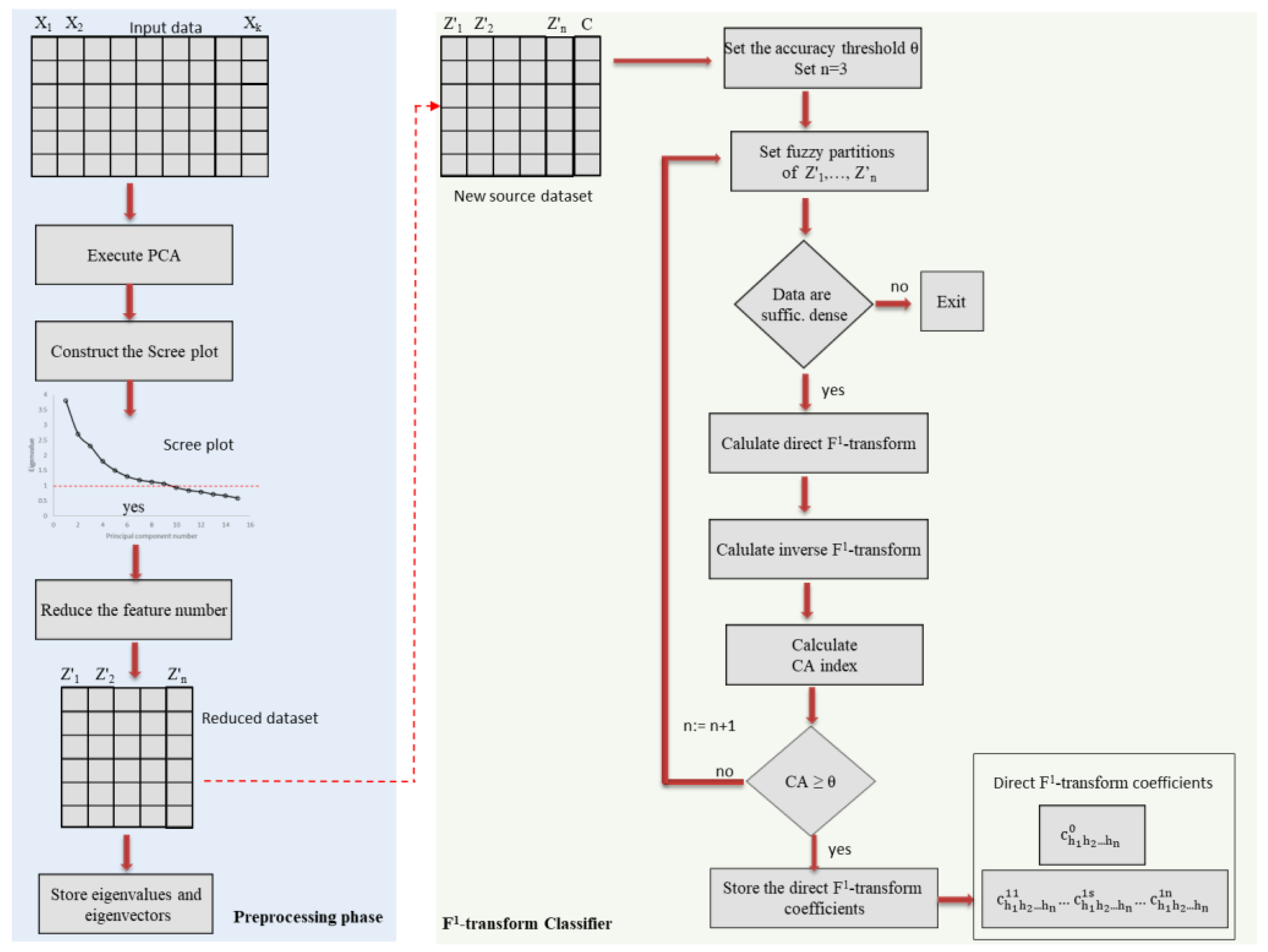
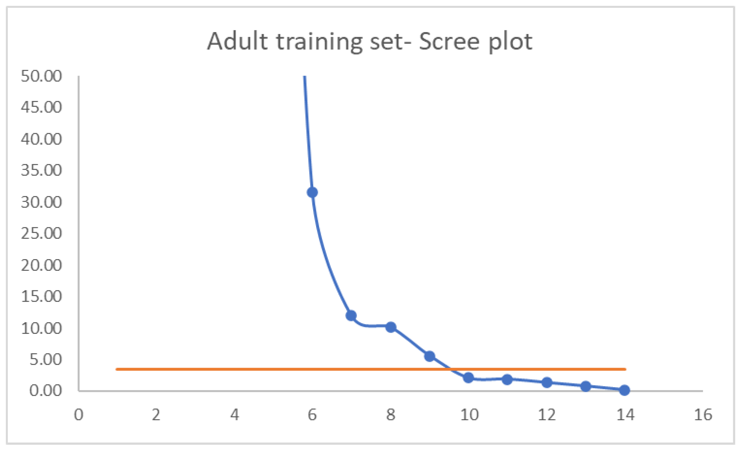
The significant principal components are selected by analyzing the eigenvalues, sorted in descending order. Three heuristic criteria are generally used for the choice of the number of components:

-

Select only the main components corresponding to the eigenvalues whose sum, compared to the sum of all the eigenvalues, is greater than or equal to a specific threshold, for example, 80% or 90%.

-

Adopt the Kaiser criterion, in which only those components are selected which correspond to an eigenvalue greater than or equal to 1, or, equivalently, the components that have variance greater than the average.

-

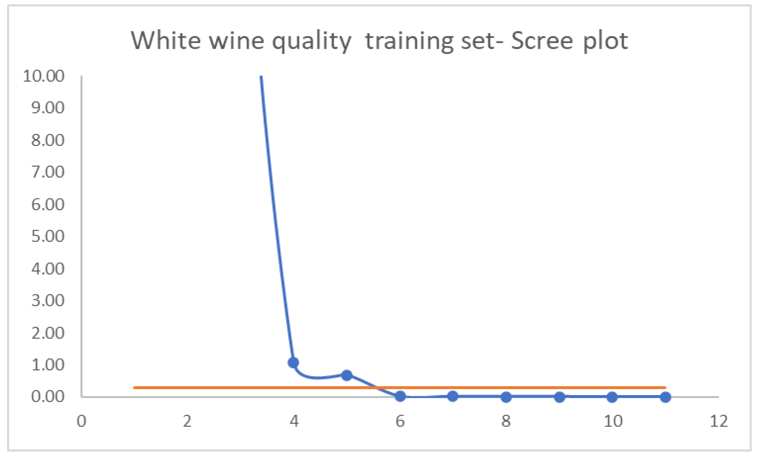
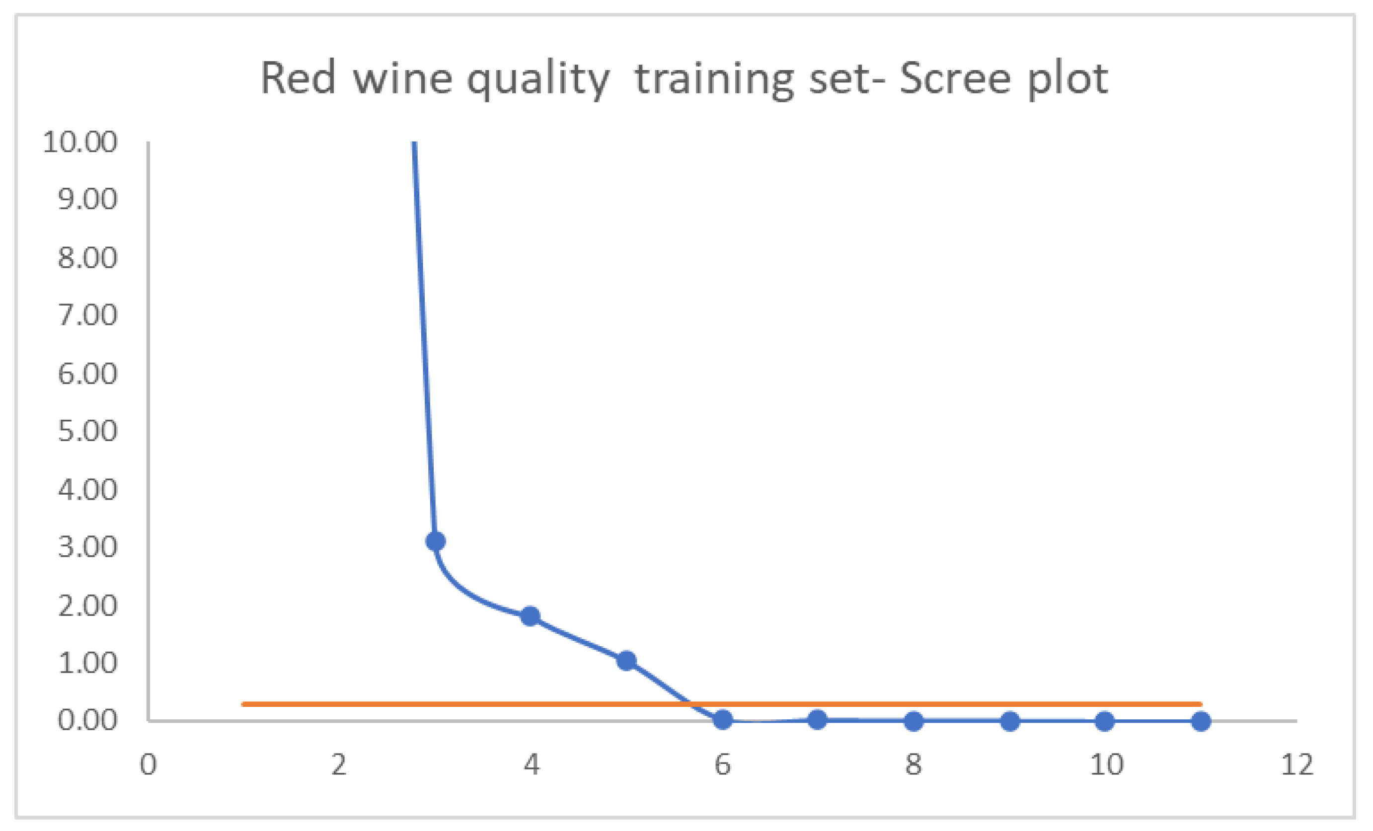
Build the eigenvalue graph, called Scree Plot, and select the number of components corresponding to the elbow point beyond which the graph the eigenvalues stabilizes.

8.

The reduced dataset is constructed considering only the significant principal components.

2.2. Multidimensional F-Transform

Let f: X ⊆ Rⁿ → Y⊆ R be a continuous n-dimensional function defined in a closed interval X = [a₁,b₁] × [a₂,b₂] ×…× [a_n,b_n] ⊆ Rⁿ and known in a discrete set of N points P = {(p₁₁, p₁₂, …, p_1n), (p₂₁, p₂₂, …, p_2n),…, (p_N1, p_N2, …,p_Nn)}.

For each i = 1,…,n let x_i1, x_i2, …, x_imi with m_i ≥ 2 be a set of m_i points of [a_i,b_i], called nodes, such that x_i1 = a_i < x_i2 <…< x_imi = b_i.

For each i = 1,…,n let A_i1, A_i2,…, A_imi: [a_i, b_i] → [0,1] be a family of fuzzy sets forming a fuzzy partition of [a_i,b_i], where:

• A_ih(x_ih) = 1 for every h =1,2,…, m_i;
• A_ih(x) = 0 if x is not in (x_ih−1, x_ih+1), where we assume x_i0 = x_i1 = a_i and x_in+1 = x_in = b_i by commodity of presentation;
• A_ih(x) strictly increases on [x_ih−1, x_ih] for h =2,…, m_i and strictly decreases on [x_ih, x_ih+1] for h = 1,…, m_i − 1;
• ${{\displaystyle \sum }}_{\mathrm{h}=1}^{{\mathrm{m}}_{\mathrm{i}}}{\mathrm{A}}_{\mathrm{ih}}\left(\mathrm{x}\right)=1$ for every x ∊ [a_i, b_i].

The fuzzy sets A_i1, A_i2,…, A_imi are called basic functions.

Let c_i = (b_i − a_i)/(m_i − 1). The basic functions A_i1, A_i2,…, A_imi form a uniform fuzzy partition of [a_i,b_i] if:

5.

m_i ≥ 3 and the nodes are equidistant, i.e., x_ih = a_i + d_i ∙ (h − 1), where d_i = (b_i − a_i)/(m_i − 1) and h = 1, 2, …, m_i.

6.

A_ih(x_ih − x) = A_ih(x_ih + x) ∀ x ∊ [0,h] and ∀ h = 2,…, m_i − 1;

7.

A_ih + 1(x) = A_ih(x − d_i) ∀ x ∊ [x_ih, x_ih + 1] and ∀ h = 1,2,…, m_i − 1.

We say that the set P = {(p₁₁, p₁₂, …, p_1n), (p₂₁, p₂₂, …, p_2n),…,(p_N1, p_N2, …,p_Nn)} is sufficiently dense w.r.t. the set of fuzzy partitions $\left\{{\mathrm{A}}_{11}{\mathrm{A}}_{12}\dots {\mathrm{A}}_{1{\mathrm{m}}_1}\right\}$,…,$\left\{{\mathrm{A}}_{\mathrm{i}1}{\mathrm{A}}_{\mathrm{i}2}\dots {\mathrm{A}}_{{\mathrm{im}}_{\mathrm{i}}}\right\}$,…, $\left\{{\mathrm{A}}_{\mathrm{n}1}{\mathrm{A}}_{\mathrm{n}2}\dots {\mathrm{A}}_{{\mathrm{nm}}_{\mathrm{n}}}\right\}$ if for each combination ${\mathrm{A}}_{1{\mathrm{h}}_1}{\mathrm{A}}_{2{\mathrm{h}}_2}\dots {\mathrm{A}}_{{\mathrm{nh}}_{\mathrm{n}}}$ exists at least a point p_j = $\left({\mathrm{p}}_{\mathrm{j}1}, {\mathrm{p}}_{\mathrm{j}2},\cdots ,{\mathrm{p}}_{\mathrm{j}\mathrm{n}}\right)$ ∊ P, such that ${\mathrm{A}}_{1{\mathrm{h}}_1}\left({\mathrm{p}}_{\mathrm{j}1}\right)\cdot {\mathrm{A}}_{2{\mathrm{h}}_2}\left({\mathrm{p}}_{\mathrm{j}2}\right)\cdot \dots \cdot {\mathrm{A}}_{{\mathrm{nh}}_{\mathrm{n}}}\left({\mathrm{p}}_{\mathrm{jn}}\right)$ > 0. In this case, we can define the direct multidimensional F-transform of f with the (h₁,h₂,…,h_s)th component ${\mathrm{F}}_{{\mathrm{h}}_1{\mathrm{h}}_2\dots {\mathrm{h}}_{\mathrm{n}}}$ given by

$${\mathrm{F}}_{{\mathrm{h}}_1{\mathrm{h}}_2\dots {\mathrm{h}}_{\mathrm{n}}}=\frac{{{\displaystyle \sum }}_{\mathrm{j}=1}^{\mathrm{N}}f\left({\mathrm{p}}_{\mathrm{j}1},{\mathrm{p}}_{\mathrm{j}2},\dots {\mathrm{p}}_{\mathrm{jn}}\right)\cdot {\mathrm{A}}_{1{\mathrm{h}}_1}\left({\mathrm{p}}_{\mathrm{j}1}\right)\cdot {\mathrm{A}}_{2{\mathrm{h}}_2}\left({\mathrm{p}}_{\mathrm{j}2}\right)\cdot \dots \cdot {\mathrm{A}}_{{\mathrm{nh}}_{\mathrm{n}}}\left({\mathrm{p}}_{\mathrm{jn}}\right)}{{{\displaystyle \sum }}_{\mathrm{j}=1}^{\mathrm{N}}{\mathrm{A}}_{1{\mathrm{h}}_1}\left({\mathrm{p}}_{\mathrm{j}1}\right)\cdot {\mathrm{A}}_{2{\mathrm{h}}_2}\left({\mathrm{p}}_{\mathrm{j}2}\right)\cdot \dots \cdot {\mathrm{A}}_{{\mathrm{nh}}_{\mathrm{n}}}\left({\mathrm{p}}_{\mathrm{jn}}\right)}$$

(5)

The multidimensional inverse F-transform, calculated in the point p_j, is given by:

$$f_{{\mathrm{n}}_1{\mathrm{n}}_2\dots {\mathrm{n}}_{\mathrm{s}}}^{\mathrm{F}}\left({\mathrm{p}}_{\mathrm{j}1},{\mathrm{p}}_{\mathrm{j}2},\dots ,{\mathrm{p}}_{\mathrm{jn}}\right)={\displaystyle {\displaystyle \sum }_{{\mathrm{h}}_1=1}^{{\mathrm{m}}_1}}{\displaystyle {\displaystyle \sum }_{{\mathrm{h}}_2=1}^{{\mathrm{m}}_2}}\dots {\displaystyle {\displaystyle \sum }_{{\mathrm{h}}_{\mathrm{n}}=1}^{{\mathrm{m}}_{\mathrm{n}}}}{\mathrm{F}}_{{\mathrm{h}}_1{\mathrm{h}}_2\dots {\mathrm{h}}_{\mathrm{n}}}\cdot {\mathrm{A}}_1{}_{{\mathrm{h}}_1}\left({\mathrm{p}}_{\mathrm{j}1}\right)\cdot \dots \cdot {\mathrm{A}}_{\mathrm{n}}{}_{{\mathrm{h}}_{\mathrm{n}}}\left({\mathrm{p}}_{\mathrm{jn}}\right)$$

(6)

It approximates the function f in the point p_j. In [11,12] the multidimensional inverse F-transform (6) is applied in regression analysis to find dependencies between attributes in datasets.

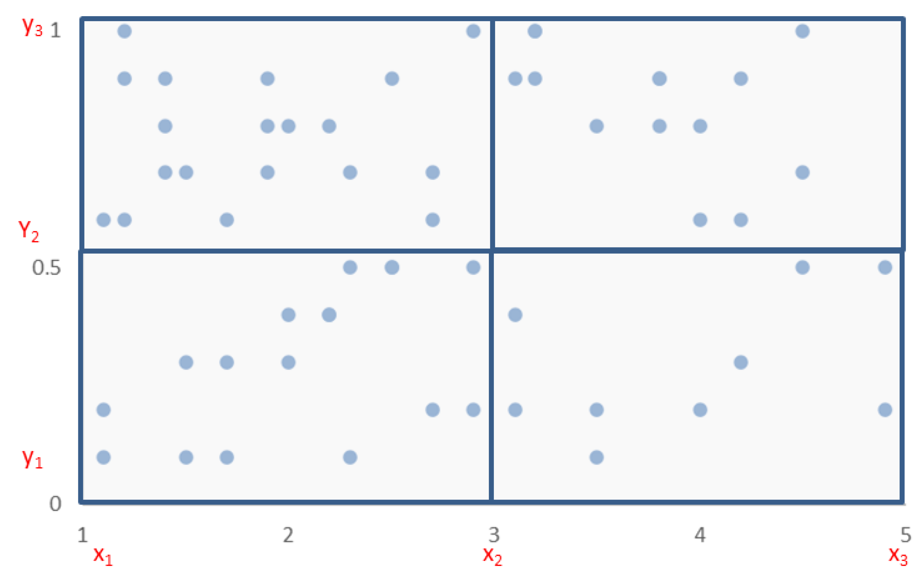
To highlight the use of the multidimensional F-transform, consider, as an example, a dataset, given by two input features defined in the close intervals, respectively, [1.1, 4.9] and [0.1, 1.0].

Suppose we create for each of the two input variables a fuzzy partition consisting of three basic functions, setting m₁ = 3 and m₂ = 3. We obtain c₁ = 1.9 and c₂ = 0.45.

Table 1. Set of nodes of the two input variables in the example.

Input Variable	Node	Value
First variable	x1	1.1
	x2	3.0
	x3	4.9
Second variable	y1	0.1
	y2	0.55
	y3	1.0

shows the values of the three nodes for the two input variables.

Figure 1 shows the points in the input variable plane. The four rectangles are drawn to show that the dataset is sufficiently dense with respect to the set of the two fuzzy partitions {A₁₁, A₁₂, A_i3} and partitions {A₂₁, A₂₂, A₂₃}. In fact, in each rectangle in the figure, there is at least one point; this implies that for every combination of basic functions A_1i, A_2i i = 1,2,3, there exists at least one point p_j = (p_j1,p_j2) such that A_1i (p_j1) A_2i (p_j1) ≠ 0.

Since the data are sufficiently dense with respect to the sets of fuzzy partitions, it is possible to apply Equation (5) to calculate the components of the multidimensional direct F-transform F_h1h2 h₁, h₂ = 1,2,3. Finally, Equation (6) can be applied to calculate the multidimensional inverse F-transform in a point p; it approximates the function f in that point.

2.3. High Degree F-Transform

This paragraph introduces the concept of higher degree fuzzy transform or F^r-transform. One-dimensional square-integrable functions will now be considered.

Let A_h, h = 1,…,n, be the hth basic function defined on [a,b] and L₂([x_h−1,x_h+1]) be the Hilbert space of square-integrable functions f,g: [x_h−1,x_h+1] ⟶ R with the inner product:

$$⟨f,g_h⟩=\frac{{{\displaystyle \int }}_{{\mathrm{x}}_{\mathrm{h}-1}}^{{\mathrm{x}}_{\mathrm{h}+1}}f\left(\mathrm{x}\right)g\left(\mathrm{x}\right){\mathrm{A}}_{\mathrm{k}}\left(\mathrm{x}\right)\mathrm{dx}}{{{\displaystyle \int }}_{{\mathrm{x}}_{\mathrm{h}-1}}^{{\mathrm{x}}_{\mathrm{h}+1}}{\mathrm{A}}_{\mathrm{h}}\left(\mathrm{x}\right)\mathrm{dx}}$$

(7)

Let L^r₂([x_h−1,x_h+1]), with r positive integer, be a linear subspace of the Hilbert space L₂([x_h−1,x_h+1]) with orthogonal basis given by polynomials {P⁰_h, P¹_h,…,P^r_h} obtained applying the Gram-Schmidt orthonormalization to the linear independent system of polynomials {1, x, x²,…, x^r} defined in the interval [x_h−1,x_h+1]. We have:

$$\left\{\begin{array}{l}{\mathrm{P}}_{\mathrm{h}}^0=1\\ {\mathrm{P}}_{\mathrm{h}}^{\mathrm{s}+1}={\mathrm{x}}^{\mathrm{s}+1}-{\displaystyle {\displaystyle \sum }_{\mathrm{j}=1}^{\mathrm{s}}}\frac{⟨{\mathrm{x}}^{\mathrm{s}+1},{\mathrm{P}}_{\mathrm{h}}^{\mathrm{j}}⟩}{⟨{\mathrm{P}}_{\mathrm{h}}^{\mathrm{j}},{\mathrm{P}}_{\mathrm{h}}^{\mathrm{j}}⟩}\end{array}\right. \mathrm{s}=1,\dots ,\mathrm{r}-1$$

(8)

The following Lemma holds (Cfr. Perfilieva et al., 2011 [3], Lemma 1):

Lemma 1.

Let$F_k^r$be the orthogonal projection of the function f on L^r₂([x_h−1,x_h+1]). Then:

$$F_h^r\left(x\right)={\displaystyle {\displaystyle \sum }_{s=1}^r}{c}_{h,i}{P}_h^s\left(x\right)$$

(9)

where

$${\mathrm{c}}_{\mathrm{h},\mathrm{s}}=\frac{⟨\mathrm{f},{\mathrm{P}}_{\mathrm{kh}}^{\mathrm{s}}⟩{}_{\mathrm{k}}}{⟨{\mathrm{P}}_{\mathrm{h}}^{\mathrm{s}},{\mathrm{P}}_{\mathrm{h}}^{\mathrm{s}}⟩{}_{\mathrm{h}}}=\frac{{{\displaystyle \int }}_{{\mathrm{x}}_{\mathrm{k}-1}}^{{\mathrm{x}}_{\mathrm{k}+1}}f\left(\mathrm{x}\right){\mathrm{P}}_{\mathrm{h}}^{\mathrm{s}}\left(\mathrm{x}\right){\mathrm{A}}_{\mathrm{h}}\left(\mathrm{x}\right)\mathrm{dx}}{{{\displaystyle \int }}_{{\mathrm{x}}_{\mathrm{k}-1}}^{{\mathrm{x}}_{\mathrm{k}+1}}{\left({\mathrm{P}}_{\mathrm{h}}^{\mathrm{s}}\left(\mathrm{x}\right)\right)}^2{\mathrm{A}}_{\mathrm{h}}\left(\mathrm{x}\right)\mathrm{dx}}$$

(10)

${\mathrm{F}}_{\mathrm{h}}^{\mathrm{r}}$ it is the h-th component of the direct F^r-transform of f F^r[f] = (F^r₁, F^r₂,_…,F^r_n).

The inverse F^r-transform of f in a point x ∊ [a,b] is:

$$f_{\mathrm{F},\mathrm{n}}^{\mathrm{r}}\left(\mathrm{x}\right)={\displaystyle \sum }_{\mathrm{k}=1}^{\mathrm{n}}{\mathrm{F}}_{\mathrm{h}}^{\mathrm{r}}{\mathrm{A}}_{\mathrm{k}}\left(\mathrm{x}\right)$$

(11)

For r = 0 we have P⁰_h = 1 and the F⁰-transform is given by the F-transform in one variable (F⁰_h(x) = c_h,0).

For r = 1 we have P¹_h = (x − x_h) and the h-th component of the F¹-transform is given by the formula:

F¹_h(x) = c_h,0 + c_h,1 (x − x_h) = F⁰_h(x) + c_h,1 (x − x_h)

(12)

If the function f is known in a set of N data points p₁,…p_N, c_h,0 and c_h,1 can be discretized in the form:

$${\mathrm{c}}_{\mathrm{h},0}=\frac{{{\displaystyle \sum }}_{\mathrm{i}=1}^{\mathrm{n}}f\left({\mathrm{p}}_{\mathrm{i}}\right){\mathrm{A}}_{\mathrm{h}}\left({\mathrm{p}}_{\mathrm{i}}\right)}{{{\displaystyle \sum }}_{\mathrm{i}=1}^{\mathrm{n}}{\mathrm{A}}_{\mathrm{h}}\left({\mathrm{p}}_{\mathrm{i}}\right)}$$

(13)

$${\mathrm{c}}_{\mathrm{k},1}=\frac{{{\displaystyle \sum }}_{\mathrm{i}=1}^{\mathrm{n}}f\left({\mathrm{p}}_{\mathrm{i}}\right)\left({\mathrm{p}}_{\mathrm{i}}-{\mathrm{x}}_{\mathrm{h}}\right){\mathrm{A}}_{\mathrm{h}}\left({\mathrm{p}}_{\mathrm{i}}\right)}{{{\displaystyle \sum }}_{\mathrm{i}=1}^{\mathrm{n}}{\mathrm{A}}_{\mathrm{h}}\left({\mathrm{p}}_{\mathrm{i}}\right){\left({\mathrm{p}}_{\mathrm{i}}-{\mathrm{x}}_{\mathrm{h}}\right)}^2}$$

(14)

Likewise, let L₂ ([x_k1−1, x_k1+1] × [x_k2−1,x_k2+1] ×…× [x_kn−1, x_kn+1]) be the Hilbert space of square- integrable n-variables functions f: [x_k1−1, x_k1+1] × [x_k2−1,x_k2+1] ×…× [x_kn−1, x_kn+1] → R with the weighted inner product:

$$f,g_{{\mathrm{h}}_1{\mathrm{h}}_2\cdots {\mathrm{h}}_{\mathrm{n}}}=\underset{{\mathrm{x}}_{{\mathrm{h}}_1-1}}{\overset{{\mathrm{x}}_{{\mathrm{h}}_1+1}}{{\displaystyle \int }}}\underset{{\mathrm{x}}_{{\mathrm{h}}_2-1}}{\overset{{\mathrm{x}}_{{\mathrm{h}}_2+1}}{{\displaystyle \int }}}\cdots \underset{{\mathrm{x}}_{{\mathrm{h}}_{\mathrm{n}}-1}}{\overset{{\mathrm{x}}_{{\mathrm{h}}_{\mathrm{n}}+1}}{{\displaystyle \int }}}f\left({\mathrm{x}}_1,{\mathrm{x}}_2,\cdots ,{\mathrm{x}}_{\mathrm{n}}\right)g\left({\mathrm{x}}_1,{\mathrm{x}}_2,\cdots ,{\mathrm{x}}_{\mathrm{n}}\right){\mathrm{A}}_{{\mathrm{h}}_1}\left({\mathrm{x}}_1\right){\mathrm{A}}_{{\mathrm{h}}_2}\left({\mathrm{x}}_2\right)\cdots {\mathrm{A}}_{{\mathrm{h}}_{\mathrm{n}}}\left({\mathrm{x}}_{\mathrm{n}}\right){\mathrm{dx}}_1\cdots {\mathrm{dx}}_{\mathrm{n}}$$

(15)

Two function $f,g\in$ L₂([x_h1−1, x_h1+1] × [x_h2−1,x_h2+1] ×…× [x_hn−1, x_hn+1]) are orthogonal if $⟨f,{g⟩}_{h_1{h}_2\cdots h_n}=0$.

Let f: X ⊆ Rⁿ → Y⊆ R be a continuous n-dimensional function defined in a closed set [a₁,b₁] × [a₂,b₂] ×…× [a_n,b_n]. Let A_hk, k = 1,…,n_k, be the kth basic function defined on the interval [a_h,b_h] and L₂([x_h,k−1,x_h,k+1]) be the Hilbert space of square-integrable functions f,g: [x_h,k−1,x_h,k+1] ⟶ R.

The inverse F¹-transform of f in a point x = (x₁, x₂,…, x_n) ∊ [a₁,b₁] × [a₂,b₂] ×…× [a_n,b_n] is:

$$f_{\mathrm{F},\mathrm{n}}^1\left(\mathrm{x}\right)={\displaystyle {\displaystyle \sum }_{{\mathrm{h}}_1=1}^{{\mathrm{m}}_1}}{\displaystyle {\displaystyle \sum }_{{\mathrm{h}}_2=1}^{{\mathrm{m}}_2}}\dots {\displaystyle {\displaystyle \sum }_{{\mathrm{h}}_{\mathrm{n}}=1}^{{\mathrm{m}}_{\mathrm{n}}}}{\mathrm{F}}_{{\mathrm{h}}_1{\mathrm{h}}_2\dots {\mathrm{h}}_{\mathrm{n}}}^1\cdot {\mathrm{A}}_1{}_{{\mathrm{h}}_1}\left({\mathrm{x}}_1\right)\cdot \dots \cdot {\mathrm{A}}_{\mathrm{n}}{}_{{\mathrm{h}}_{\mathrm{n}}}\left({\mathrm{x}}_{\mathrm{n}}\right)$$

(16)

where ${\mathrm{F}}_{{\mathrm{h}}_1{\mathrm{h}}_2\dots {\mathrm{h}}_{\mathrm{n}}}^1\left(\mathrm{x}\right)$ is the (h₁, h₂,…, h_n)th component of the direct F¹-transform, given by the formula:

$${\mathrm{F}}_{{\mathrm{h}}_1{\mathrm{h}}_2\dots {\mathrm{h}}_{\mathrm{n}}}^1\left(\mathrm{x}\right)={\mathrm{c}}_{{\mathrm{h}}_1{\mathrm{h}}_2\dots {\mathrm{h}}_{\mathrm{n}}}^0+{\displaystyle {\displaystyle \sum }_{\mathrm{s}=1}^{\mathrm{n}}}{\mathrm{c}}_{{\mathrm{h}}_1{\mathrm{h}}_2\dots {\mathrm{h}}_{\mathrm{n}}}^{1\mathrm{s}}\cdot \left({\mathrm{x}}_{\mathrm{s}}-{\mathrm{x}}_{{\mathrm{h}}_{\mathrm{t}}}\right)$$

(17)

If f is known in a set of N n-dimensional data points p₁,…p_N where p_i = (p_i1, p_i2,…, p_in), we obtain:

$${\mathrm{c}}_{{\mathrm{h}}_1{\mathrm{h}}_2\dots {\mathrm{h}}_{\mathrm{n}}}^0={\mathrm{F}}_{{\mathrm{h}}_1{\mathrm{h}}_2\dots {\mathrm{h}}_{\mathrm{n}}}=\frac{{{\displaystyle \sum }}_{\mathrm{j}=1}^{\mathrm{N}}f\left({\mathrm{p}}_{\mathrm{j}1},{\mathrm{p}}_{\mathrm{j}2},\dots {\mathrm{p}}_{\mathrm{jn}}\right)\cdot {\mathrm{A}}_{1{\mathrm{h}}_1}\left({\mathrm{p}}_{\mathrm{j}1}\right)\cdot {\mathrm{A}}_{2{\mathrm{h}}_2}\left({\mathrm{p}}_{\mathrm{j}2}\right)\cdot \dots \cdot {\mathrm{A}}_{{\mathrm{nh}}_{\mathrm{n}}}\left({\mathrm{p}}_{\mathrm{jn}}\right)}{{{\displaystyle \sum }}_{j=1}^{\mathrm{N}}{\mathrm{A}}_{1{\mathrm{h}}_1}\left({\mathrm{p}}_{\mathrm{j}\mathrm{1}}\right)\cdot {\mathrm{A}}_{2{\mathrm{h}}_2}\left({\mathrm{p}}_{\mathrm{j}2}\right)\cdot \dots \cdot {\mathrm{A}}_{\mathrm{n}{\mathrm{h}}_{\mathrm{n}}}\left({\mathrm{p}}_{\mathrm{j}\mathrm{n}}\right)}$$

(18)

$${\mathrm{c}}_{{\mathrm{h}}_1{\mathrm{h}}_2\dots {\mathrm{h}}_{\mathrm{n}}}^{1\mathrm{s}}=\frac{{{\displaystyle \sum }}_{\mathrm{j}=1}^{\mathrm{N}}f\left({\mathrm{p}}_{\mathrm{j}1},{\mathrm{p}}_{\mathrm{j}2},\dots {\mathrm{p}}_{\mathrm{jn}}\right)\cdot \left({\mathrm{p}}_{\mathrm{js}}-{\mathrm{x}}_{{\mathrm{h}}_{\mathrm{s}}}\right)\cdot {\mathrm{A}}_{1{\mathrm{h}}_1}\left({\mathrm{p}}_{\mathrm{j}1}\right)\cdot {\mathrm{A}}_{2{\mathrm{h}}_2}\left({\mathrm{p}}_{\mathrm{j}2}\right)\cdot \dots \cdot {\mathrm{A}}_{{\mathrm{nh}}_{\mathrm{n}}}\left({\mathrm{p}}_{\mathrm{jn}}\right)}{{{\displaystyle \sum }}_{\mathrm{j}=1}^{\mathrm{N}}{\left({\mathrm{p}}_{\mathrm{js}}-{\mathrm{x}}_{{\mathrm{h}}_{\mathrm{s}}}\right)}^2\cdot {\mathrm{A}}_{1{\mathrm{h}}_1}\left({\mathrm{p}}_{\mathrm{j}1}\right)\cdot {\mathrm{A}}_{2{\mathrm{h}}_2}\left({\mathrm{p}}_{\mathrm{j}2}\right)\cdot \dots \cdot {\mathrm{A}}_{{\mathrm{nh}}_{\mathrm{n}}}\left({\mathrm{p}}_{\mathrm{jn}}\right)}$$

(19)

where ${\mathrm{c}}_{{\mathrm{h}}_1{\mathrm{h}}_2\dots {\mathrm{h}}_{\mathrm{n}}}^0$ is the component ${\mathrm{F}}_{{\mathrm{h}}_1{\mathrm{h}}_2\dots {\mathrm{h}}_{\mathrm{n}}}$of the multidimensional discrete direct F transform of f, given by (5).

3. The F¹-Transform Classification Method

The proposed classification method executes the multidimensional F¹-transform to classify data points. The method is schematized in Figure 2.

In a pre-processing phase, PCA is executed in order to reduce the number of features. The scree plot method is applied to detect the principal components. The eigenvalues are sorted in ascending order to create the Scree Plot; then, the elbow point is set; the features corresponding to the eigenvalues under the elbow point on the y-axis will be deleted. Output of the pre-processing phase is the new reduced dataset in the transformed coordinates.

The F¹-transform classifier follows the strategy adopted in the MFC algorithm [14]. Initially the classification accuracy threshold is set to θ and coarse-grained fuzzy partitions are created (n = 3). After creating the fuzzy partitions of the domains of each feature the algorithm checks that the data are sufficiently dense with respect to the fuzzy partitions; if they are, then the direct and inverse F¹-transforms are computed, otherwise, the algorithm terminates because the cardinality of the fuzzy partitions is too fine compared to the density of data points in the feature space and the direct F¹-transform cannot be computed.

The Calculate CA index component measures the accuracy of the classification. To classify a data point we adopt the following method applied in [9].

Let C be the number of classes and let l₁, l₂,…, l_C be the labels of the C classes. Let p_j = (p_j1, p_j2,…, p_jn, m_j) the jth data point, where m_j is the position of the corresponding class.

The components of the F1-transform (18) and (19) are given by:

$${\mathrm{c}}_{{\mathrm{h}}_1{\mathrm{h}}_2\dots {\mathrm{h}}_{\mathrm{n}}}^0={\mathrm{F}}_{{\mathrm{h}}_1{\mathrm{h}}_2\dots {\mathrm{h}}_{\mathrm{n}}}=\frac{{{\displaystyle \sum }}_{\mathrm{j}=1}^{\mathrm{N}}{\mathrm{m}}_{\mathrm{j}}\cdot {\mathrm{A}}_{1{\mathrm{h}}_1}\left({\mathrm{p}}_{\mathrm{j}1}\right)\cdot {\mathrm{A}}_{2{\mathrm{h}}_2}\left({\mathrm{p}}_{\mathrm{j}2}\right)\cdot \dots \cdot {\mathrm{A}}_{{\mathrm{nh}}_{\mathrm{n}}}\left({\mathrm{p}}_{\mathrm{jn}}\right)}{{{\displaystyle \sum }}_{\mathrm{j}=1}^{\mathrm{N}}{\mathrm{A}}_{1{\mathrm{h}}_1}\left({\mathrm{p}}_{\mathrm{j}1}\right)\cdot {\mathrm{A}}_{2{\mathrm{h}}_2}\left({\mathrm{p}}_{\mathrm{j}2}\right)\cdot \dots \cdot {\mathrm{A}}_{\mathrm{n}{\mathrm{h}}_{\mathrm{n}}}\left({\mathrm{p}}_{\mathrm{j}\mathrm{n}}\right)}$$

(20)

$${\mathrm{c}}_{{\mathrm{h}}_1{\mathrm{h}}_2\dots {\mathrm{h}}_{\mathrm{n}}}^{1\mathrm{s}}=\frac{{{\displaystyle \sum }}_{\mathrm{j}=1}^{\mathrm{N}}{\mathrm{m}}_{\mathrm{j}}\cdot \left({\mathrm{p}}_{\mathrm{js}}-{\mathrm{x}}_{{\mathrm{h}}_{\mathrm{s}}}\right)\cdot {\mathrm{A}}_{1{\mathrm{h}}_1}\left({\mathrm{p}}_{\mathrm{j}1}\right)\cdot {\mathrm{A}}_{2{\mathrm{h}}_2}\left({\mathrm{p}}_{\mathrm{j}2}\right)\cdot \dots \cdot {\mathrm{A}}_{{\mathrm{nh}}_{\mathrm{n}}}\left({\mathrm{p}}_{\mathrm{jn}}\right)}{{{\displaystyle \sum }}_{\mathrm{j}=1}^{\mathrm{N}}{\left({\mathrm{p}}_{\mathrm{js}}-{\mathrm{x}}_{{\mathrm{h}}_{\mathrm{s}}}\right)}^2\cdot {\mathrm{A}}_{1{\mathrm{h}}_1}\left({\mathrm{p}}_{\mathrm{j}1}\right)\cdot {\mathrm{A}}_{2{\mathrm{h}}_2}\left({\mathrm{p}}_{\mathrm{j}2}\right)\cdot \dots \cdot {\mathrm{A}}_{{\mathrm{nh}}_{\mathrm{n}}}\left({\mathrm{p}}_{\mathrm{jn}}\right)}$$

(21)

Let $f_{\mathrm{F},\mathrm{n}}^1\left({\mathrm{p}}_{\mathrm{j}}\right)$ the inverse F¹-transform computed by (16). The index of the class assigned to the data point p_j is given by an integer $\widehat{{\mathrm{m}}_{\mathrm{j}}}$in {1,2,…,C} given by:

$$\widehat{{\mathrm{m}}_{\mathrm{j}}}=\left[\underset{\mathrm{m}=1,\dots ,\mathrm{C}}{\min }\left(\left|{\mathrm{f}}_{\mathrm{F},\mathrm{n}}^1({\mathrm{p}}_{\mathrm{j}})-\mathrm{m}\right|\right)\right]$$

(22)

where [a] stands for the greatest integer containing the positive real number a.

The classification accuracy CA is given by the ratio between the number of data points correctly classified and the total number of data points.

If CA is less than the threshold θ, then finer fuzzy partitions with n + 1 fuzzy sets are created and the process is iterated. Otherwise, the F¹-transform classifier ends, storing the coefficients of the final direct F¹-transform: ${\mathrm{c}}_{{\mathrm{h}}_1{\mathrm{h}}_2\dots {\mathrm{h}}_{\mathrm{n}}}^0$ and ${\mathrm{c}}_{{\mathrm{h}}_1{\mathrm{h}}_2\dots {\mathrm{h}}_{\mathrm{n}}}^{11}\cdots {\mathrm{c}}_{{\mathrm{h}}_1{\mathrm{h}}_2\dots {\mathrm{h}}_{\mathrm{n}}}^{1\mathrm{n}}$ computed, respectively by (18) and (19).

A new input data x = (x₁, x₂,…, x_n) will be classified computing the inverse F¹-transform $f_{\mathrm{F},\mathrm{n}}^1\left(\mathrm{x}\right)$ by (16) and assigning it the wth class by (20).

The F¹-transform classification algorithm is schematized below (Algorithm 1):

Algorithm 1. F1-transform classification

Execute the PCA feature reduction algorithm Use the Scree plot method to reduce the number of features Create the reduced dataset Set the accuracy threshold θ n:=3 CA:=0 // initialize the CA index to 0 While CA < θ Create the n-size fuzzy partitions of the feature domains If data are sufficiently dense with respect to the n-dimensional fuzzy partitions Then Calculate the direct F1-transform by (17) Calculate the inverse F1-transform by (16) Calculate the CA index If CA ≥ θ Then Store the direct F1-transform coefficients ${\mathrm{c}}_{{\mathrm{h}}_1{\mathrm{h}}_2\mathrm{\dots }{\mathrm{h}}_{\mathrm{n}}}^0$ and ${\mathrm{c}}_{{\mathrm{h}}_1{\mathrm{h}}_2\mathrm{\dots }{\mathrm{h}}_{\mathrm{n}}}^{11}\cdots {\mathrm{c}}_{{\mathrm{h}}_1{\mathrm{h}}_2\mathrm{\dots }{\mathrm{h}}_{\mathrm{n}}}^{1\mathrm{n}}$ 15. Return “Data classified” 16. End if 17. ld>17. Else 18. Return “Data cannot be classified” 19. ld>19. End if 20. n:= n+1 21. End While

4. Experimental Results

We tested the F1-transform classification method on various classification datasets extracted from the UC Irvine Machine Learning Repository.

Table 2. Datasets in the UCI machine learning datasets used in the comparison analysis.

Dataset	Number of Data Points	Number of Features
Adult	48,842	14
Balance Scale	625	4
Bank Marketing	41,188	17
Breast cancer	286	9
Echocardiogram	132	12
Ecoli	336	7
Heart disease	303	14
Hepatitis	155	19
Thyroid disease	7200	21
Wine quality—red wine	1599	12
Wine quality—white wine	4898	12

shows the size and the number of features of the classification datasets used in these comparison tests.

To measure the classification performances, we compared the F¹-transform method with the Support Vector Machine (SVM) [24], Random Forest (RF) [25], Artificial Neural Network (ANN) [26], and the MFC classification algorithm (MFC) [14].

Our comparison tests were executed using an Intel Core I7 processor having a 5.4 GHz clock frequency.

After removing ambiguous data points, each dataset was randomly segmented into a training and a test set, containing 80% and 20% of the data points, respectively.

While running RF the number of decision trees is set to 100. The Radial Basis kernel function is used to execute SVM, setting the parameters c and gamma, respectively, to 1.0 and 0.1. ANN is executed by constructing a network having two hidden layers, and setting to 100 the maximum number of epochs.

For brevity, we show the complete results obtained for three classification datasets: the two datasets Red and White Wine Quality and the dataset Adult.

4.1. Red and White Wine Quality Classification Dataset

The red and white wine quality datasets are two classification datasets used to classify the quality of red and white variants of the Portuguese vinho verde wine.

The data points are vectors given by 11 physicochemical features. In

Table 3. Red and white wine datasets: Description of the features.

Feature Name	Description	Type of Field
fixed acidity	tartaric acid (g/dm3)	Continuous
volatile acidity	Acetic acid (g/dm3)	Continuous
citric acid	Citric acid (g/dm3)	Continuous
residual sugar	Residual sugar (g/dm3)	Continuous
chlorides	Sodium chloride(g/dm3)	Continuous
free sulfur dioxide	Free sulfur dioxide (mg/dm3)	Continuous
total sulfur dioxide	Total sulfur dioxide (mg/dm3)	Continuous
density	Density (g/cm3)	Continuous
pH	pH	Continuous
sulphates	Potassium sulphate (g/dm3)	Continuous
alcohol	Alcohol (vol.%)	Continuous
quality	Wine quality	List (an integer from 0 to 10)

all the features are described.

The last feature, called quality, is the output feature containing the class of wine quality in a scale between 0 (very bad) to 10 (excellent).

The white wine quality dataset contains 4898 data points, and the red wine quality dataset contains 1599 data points. The two datasets are unbalanced, with over 70% of the data points classified with quality five and six. Paragraphs 4.1.1 and 4.1.2 show the results obtained, respectively, for the white and for the red wine quality datasets.

4.1.1. White Wine Quality Dataset—Classification Results

Now we show the results obtained on the white wine-quality dataset.

In the preprocessing phase, the PCA algorithm was executed on the training set. In Figure 3 the scree plot is shown. The orange line highlights the elbow point. In the transformed training set, the size of the data points is reduced from eleven to five. Then, the F¹-transform classification algorithm is executed on the transformed training set. Finally, the stored final F¹-transform coefficients are used to classify the data points in the transformed test set.

We compare the classification results with the ones obtained executing SVM, RF, ANN, and MFC on the original training set.

Table 4. White wine dataset: Classification performance comparison.

Phase	Method	Accuracy	Precision	Recall	F1-Score
Training	SVM	0.75	0.77	0.74	0.75
	RF	0.73	0.76	0.71	0.73
	ANN	0.78	0.79	0.77	0.78
	MFC	0.76	0.77	0.75	0.76
	F1-transform	0.83	0.82	0.83	0.82
Test	SVM	0.74	0.75	0.74	0.74
	RF	0.73	0.74	0.71	0.72
	ANN	0.77	0.80	0.77	0.79
	MFC	0.76	0.76	0.74	0.76
	F1-transform	0.82	0.81	0.82	0.81

shows the accuracy, precision, recall, and F1-score measures computed on the training and test sets executing the five classification methods.

The results in Table 3 show that the best performances are obtained by executing the F¹-transform classification method. The F¹-transform method improves the classification accuracy obtained by executing ANN by about 5% on the training and test sets; it improves the one obtained by executing MFC by about 7% on the training set and 6% on the test set.

4.1.2. Red Wine Quality Dataset—Classification Results

The PCA algorithm was executed on the training set. Figure 4 shows the scree plot. The orange line highlights the elbow point.

As well as for the white wine quality training set, the size of the data points in the transformed training set is reduced from eleven to five.

Table 5. Red wine dataset: Classification performance comparison.

Phase	Method	Accuracy	Precision	Recall	F1-Score
Training	SVM	0.68	0.68	0.67	0.67
	RF	0.70	0.68	0.66	0.67
	ANN	0.72	0.71	0.69	0.72
	MFC	0.69	0.69	0.68	0.69
	F1-transform	0.76	0.74	0.75	0.75
Test	SVM	0.69	0.69	0.67	0.68
	RF	0.69	0.68	0.67	0.68
	ANN	0.72	0.73	0.72	0.72
	MFC	0.70	0.70	0.71	0.70
	F1-transform	0.75	0.76	0.75	0.75

shows the Accuracy, Precision, Recall, and F1-score measures computed on the training and test sets executing the five classification methods.

The results of the tests applied on the red wine quality dataset confirm that the best performances are obtained executing the F¹-transform classification method The F¹-transform method improves the classification accuracy of MFC by about 5% on both training and test sets.

The F¹-transform method improves the classification accuracy obtained by executing ANN by about 4% on the training set and 3% on the test set; it improves the one obtained by executing MFC by about 7% on the training set and 5% on the test set.

4.2. Adult Classification Dataset

The Adult dataset contains information extracted from the United States census bureau database, which includes information on residents of various states to determine whether a citizen earns more or less than 50K USD per year.

The training set contains 32,561 unambiguous data points; the data points are vectors formed by fourteen input features, four continuous and ten categorical. The test set contains 16,282 unambiguous data points.

Table 6. Adult dataset: Description of the features.

Feature Name	Description	Type of Field
age	Age	Continuous
workclass	Work class	List
fnlwgt	Survey weight	Continuous
education	Education	List
education-num	Education number	Continuous
marital status	Marital status	List
occupation	Occupation	List
relationship	Type of relationship	List
race	Race	List
sex	Gender	List: (Female, Male)
capital-game	Capital-game	Continuous
capital-loss	Capital-loss	Continuous
hours-per-week	Hours of work per week	Continuous
native-country	Native country	List:
class	Annual income	List: (<=50 K, <50 K)

shows the description of each feature.

The output class feature, called class, assumes two values, depending on whether the person makes over 50K or under 50K USD a year. The dataset is unbalanced, where over 75% of the data points are classified with an annual income under 50K USD.

To execute F¹-transform, all the categorical features were transformed into integers assigning to each term in the list of values an integer starting from 1 to the number of unique values.

PCA is executed in order to reduce the number of features. Figure 5 shows the scree plot and the elbow point set to 2.5. The first nine components are selected and the input features are reduced from fourteen to nine.

Then, the F¹-transform classification method is applied to the reduced training set.

The comparison results with SVM, RF, ANN, and MFC are shown in

Table 7. Adult dataset: Classification performance comparison.

Phase	Method	Accuracy	Precision	Recall	F1-Score
Training	SVM	0.87	0.85	0.84	0.84
	RF	0.85	0.84	0.83	0.83
	ANN	0.88	0.86	0.86	0.86
	MFC	0.86	0.85	0.85	0.85
	F1-transform	0.93	0.89	0.90	0.89
Test	SVM	0.87	0.86	0.85	0.85
	RF	0.85	0.83	0.82	0.67
	ANN	0.88	0.87	0.86	0.86
	MFC	0.87	0.86	0.86	0.86
	F1-transform	0.92	0.91	0.90	0.90

.

Even in this case, the best performances are obtained executing F¹-transform.

The F¹-transform method improves the classification accuracy obtained by executing ANN by about 4% on the training set and 3% on the test set; it improves the one obtained by executing MFC by about 5% on the training set and 4% on the test set.

Table 8. Classification Accuracy and CPU time comparison results.

Dataset	Method	SVM	RF	ANN	MFC	F1-tr
Adult	Accuracy	0.87	0.85	0.88	0.86	0.93
	CPU time (s)	858.22	849.74	915.19	881.86	877.37
Balance scale	Accuracy	0.95	0.92	0.96	0.95	0.98
	CPU time (s)	26.48	26.19	28.41	27.63	26.92
Bank Marketing	Accuracy	0.77	0.75	0.78	0.77	0.82
	CPU time (s)	832.31	823.09	944.56	867.83	864.95
Breast cancer	Accuracy	0.90	0.88	0.91	0.90	0.94
	CPU time (s)	31.67	31.78	33.59	32.06	31.78
Diabetes	Accuracy	0.73	0.73	0.76	0.75	0.77
	CPU time (s)	44.77	43.46	47.09	45.02	44.91
Echocardiogram	Accuracy	0.75	0.73	0.75	0.74	0.78
	CPU time (s)	31.67	30.93	33.10	31.28	31.32
Ecoli	Accuracy	0.79	0.78	0.81	0.79	0.83
	CPU time (s)	32.65	32.38	34.32	32.77	32.82
Heart disease	Accuracy	0.83	0.82	0.85	0.85	0.87
	CPU time (s)	37.79	37.56	40.18	38.51	38.47
Hepatitis	Accuracy	0.88	0.89	0.91	0.89	0.93
	CPU time (s)	42.61	42.49	44.26	42.68	42.73
Thyroid disease	Accuracy	0.95	0.94	0.97	0.96	0.99
	CPU time (s)	103.34	102.85	113.93	102.98	102.87
Wine quality—red wine	Accuracy	0.68	0.70	0.72	0.69	0.76
	CPU time (s)	67.52	66.81	69.54	68.15	68.23
Wine quality—white wine	Accuracy	0.75	0.73	0.78	0.76	0.83
	CPU time (s)	58.60	58.46	59.87	58.72	58.85

shows, for each dataset, the final classification accuracy and the CPU time measured executing the five algorithms.

In all cases the F¹-transform method improves the final accuracy obtained executing SVM, RS, ANN, and MFC; the final accuracy obtained using F¹-transform improves that obtained using MFC by a value ranging between 2% (dataset Diabetes) and 7% (dataset Adult).

The CPU times employed by executing F¹-transform are compatible with the ones employed by executing the other four classification algorithms. In fact, even if the construction of the multidimensional F¹-transform in the proposed algorithm requires more computational expenditure than that necessary to construct the multidimensional F-transform in the MFC algorithm, the application of the PCA algorithm in the preprocessing phase allows for the reduction of the size of the data points, reducing, thus, the computational complexity. The results show that the F¹-transform classification method improves the classification accuracy of all other classification methods, with CPU times comparable with those of MFC. In fact, the classification accuracy of F¹-transform improves that of MFC by a value between 2% and 7% and the CPU times are similar to those obtained by running MFC.

In a nutshell, in all tests performed F¹-transform produces classification accuracy better than that obtained with other classifiers and compatible execution times. In particular, the results in Table 8 show that:

-

The F1-transform classifier improves the accuracy obtained with MFC by a percentage in the range between 2% and 7%;

-

Even if the computation times of the multidimensional F¹-transform are higher than those of the multidimensional F-transform, the proposed classification algorithm has execution times similar to those of MFC.

A possible critical point of F¹-transform consists of the choice of the elbow point in the scree plot obtained by executing the PCA method in the preprocessing phase. In all the tests performed in the scree plot obtained, there is a sudden change in slope which allows the elbow point to be easily recognized. It could happen that this trend change in the scree plot is not so evident, to the point of not allowing the precise definition of the elbow point. In these cases, the solution could be to run F¹-transform multiple times, each time choosing a different number of main components and selecting the one that produces the greatest accuracy. However, this solution can significantly increase the CPU times of the algorithm.

5. Conclusions

We propose a classification method based on the multidimensional F¹-transform in which the PCA technique is applied in the preprocessing phase to reduce the size of the features. The main aim of this research is to improve the accuracy of the MFC classification algorithm based on the multidimensional F-transform, without further increasing the processing times.

We compared the performances of the proposed classification method both with those of MFC and with those of the well-known SVM, Random Forest, and ANN classification algorithms; the comparative tests were performed on classification datasets of the UCI machine learning repository.

The results show that the multidimensional F¹-transform classification algorithm increases the classification performances obtained executing SVM, Random Forest, ANN, and MFC; in addition, the execution times are comparable with the ones obtained running MFC.

We intend to carry out future research to test the use of the classification method based on the multidimensional F¹-transform on a more extensive and varied set of datasets, adapting the method to the management of ambiguous data points.