1. Introduction
The concept of fuzzy graph had been proposed by Rosenfeld [
1] to handle indeterminate phenomena on vertices and relation between vertices. Therefore, the vertices and edges have membership degrees to represent the indeterminacy situation. In real-world problems, the degrees of non-membership of elements in a network are needed, for example, in situations that need an answer of types “yes” and “no”. To handle this problem, Atanassov [
2] proposed an intuitionistic fuzzy set (IFS) and an intuitionistic fuzzy graph (IFG). Each element in IFG has membership and non-membership degrees. Numerous studies had been conducted on intuitionistic fuzzy graphs (IFGs), including the coloring of IFGs ([
3,
4]), the application of wiener index for IFGs in water pipeline network [
5], interval-valued intuitionistic
-fuzzy graphs [
6], and interval-valued intuitionistic fuzzy competition graphs [
7].
Two categories of memberships are not always sufficient for making decisions. Therefore, Cuong [
8] proposed a picture fuzzy set where each element not only had membership and non-membership degrees but also had a neutral membership degree. For instance, in an election problem, the committee must count the number of people who chose or did not choose a candidate and how many abstained (the neutral condition). Further, the concept of a picture fuzzy graph (PFG) was developed in [
9], wherein the vertices and edges had membership, neutral, and non-membership degrees.
Researchers recently expanded PFGs in numerous types, such as q-rung PFGs [
10], balanced PFGs [
11], the application of PFGs for selecting best routes in an airlines network [
12], picture fuzzy soft graphs [
13], complex PFGs [
14], regular PFGs [
15], and so on. Numerous studies had also been conducted on the use of PFGs in practical issues such as the application of balanced PFGs [
11], decision making under picture fuzzy soft graphs [
13], the implementation of regular PFGs in communication networks [
15], road map design using picture fuzzy multigraphs [
16], the application of PFGs in social networks [
17], the shortest path algorithm in picture fuzzy digraphs [
18], the site selection problem using laplacian energy of PFGs [
19], the application of picture fuzzy tolerance graphs [
20], the genus of PFGs [
21], and multiple attribute decision-making via PFGs [
22].
The theory of vertex coloring and edge coloring had been generalized in various types of fuzzy graphs. Some researchers proposed various generalizations of graph coloring such as the coloring of fuzzy graphs based on strong and weak adjacencies [
23], fuzzy graph coloring based on
-fuzzy independent vertex sets [
24], the fuzzy fractional coloring of fuzzy graphs [
25], the fuzzy coloring of fuzzy graphs [
26], the fuzzy colouring of m-polar fuzzy graphs [
27], the chromatic number and perfectness of fuzzy graphs [
28], and the edge coloring of fuzzy graphs [
29]. Several researchers have also proposed the coloring methods through the
-cut approach and two forms of adjacencies (strong and weak) in fuzzy graphs and IFGs, as seen in [
3,
4,
23,
30]. The fact that a PFG is an extension of an IFG inspired us to generalize the vertex coloring from IFGs into PFGs in 2021 [
31]. We utilized the
-cut approach to color PFGs. However, the computation of PFG’s coloring through the cut was complicated since we should have used various values of
when determining the cut chromatic numbers. Therefore, we need another approach for coloring the PFGs.
Strong and weak adjacencies—two different forms of adjacencies—between vertices in fuzzy graphs and IFGs are crucial in decision-making issues. Hence, we generalized strong and weak adjacencies into PFGs and proposed a concept to color PFGs based on strong and weak adjacencies [
32]. When we work with PFGs with many vertices and edges, we need a computational tool to identify the strong and weak adjacencies and find the chromatic number of PFGs. In this paper, we construct an algorithm to handle the problem. In PFGs, we can classify connections between two movements (two vertices) into one of these three situations, i.e., crossing conflict, merging conflict, and non-conflict. The crowdedness of traffic flows in conflicting movements (crossing or merging conflicts) is a phenomenon that needs an answer of types “yes”, “no”, and “neutral”. The situation at an intersection is usually crowded during peak times (06.30 a.m.–08.30 a.m. and 04.00 p.m.–06.00 p.m.). However, occasionally it is not congested during non-peak hours (06.00 p.m.–06.00 a.m.) or neutral conditions about whether it is crowded or not during 08.30 a.m.–03.30 p.m. Therefore, we need a PFG to deal with this situation and propose a traffic signal phasing wherein there are no traffic flows from merging conflicts that move simultaneously at the same time. In this article, we improve the method to model traffic flows at an intersection using PFGs and to determine the traffic signal phasing. Moreover, we also evaluate the proposed method through a case study. This is a new finding in view of the application of coloring of PFGs.
The following is the structure of this paper: The first section explains an introduction, and
Section 2 discusses research challenges and gaps.
Section 3 presents preliminary materials.
Section 4 contains the most important findings in this research, and
Section 5 provides an experimental result. Finally, the conclusions are given in
Section 6.
3. Preliminaries
We review some of the key ideas from this study in this part. In the beginning, we are going to discuss intuitionistic fuzzy sets (IFSs) and the construction of an IFS from a fuzzy set.
Given an ordinary finite non-empty set X and , an Atanassov IFS on X is a set of the form wherein and for each . Meanwhile, a degree of hesitation (intuitionistic fuzzy index) of an element x in IFS is defined as .
A method to construct an IFS from a fuzzy set is given in Proposition 1, Theorem 1, and Corollary 1, which are cited from [
34,
35].
Proposition 1 ([
34,
35])
. Let F be a mapping that is defined as with , and , where and . Let be a function defined as for . The mapping F satisfies the following conditions:- 1.
If , then for ,
- 2.
for ,
- 3.
,
- 4.
,
- 5.
,
- 6.
.
Theorem 1 ([
34,
35])
. Let be a set of all fuzzy set in X and . Let be a fuzzy set in , where . Let be two functions defined on X. The setis an Atanassov IFS, where the function F is defined as in Proposition 1. Corollary 1 ([
34])
. Let and F be two functions as defined in Proposition 1. If we choose for each in Theorem 1, thenUnder the condition in Corollary 1, we obtain an IFS: The non-membership degree of IFS
in (
1) will be used in the implementation of coloring of PFGs in
Section 5.
Furthermore, the notion of a picture fuzzy set (PFS) and the construction of a PFS from an IFS are discussed.
Definition 1 ([
8])
. Given a universal set X and . A set of the form is mentioned as a PFS on X, wherein is a membership degree that describes the truth value of existence of element v in , is a NeuM degree that represents the indeterminacy degree of existence of v in , and is a non-membership degree that shows the falsity degree of existence of v in PFS , such that . The value is called a refusal degree of membership of v in . A method to construct a PFS from an IFS is given in Theorem 2.
Theorem 2 ([
36])
. If is an IFS on X and is any function such that and , thenis a PFS on X wherein the mapping is defined by with and . In other words,
,
, and
for
. Further, the function
g in Theorem 2 is called a neutral or refusal membership function of PFS
, and it will be used in
Section 5.
In Definitions 2 and 3, we present ideas of an empty PFS and a universal PFS, which are cited from [
37].
Definition 2 ([
37])
. Let be a PFS on X and . The set is called an empty PFS if , and for each . The empty PFS is denoted by . Definition 3 ([
37])
. Given PFS in Definition 2, the set is named a universal PFS if , and for each . Additionally, we provide information on the picture fuzzy subset in Definition 4, which is quoted from [
8].
Definition 4 ([
8])
. Let X be a universal set and . Given two PFSs on X: and , . The PFS is mentioned as the picture fuzzy subset of , denoted by , iffor all . The notion of PFS is used as a basis to define a PFG, as described in Definition 5.
Definition 5 ([
9])
. We assume that X is a universal set that contains vertices. We mention a graph as a PFG if is a picture fuzzy vertex set (PFVS) on X with the membership, neutral, and non-membership functions as follows: , in which for each . Meanwhile, is a picture fuzzy edge set (PFES) on with the membership, neutral membership, and non-membership functions as follows: such thatand for each . The value of is a membership degree that represents the truth value of existence of vertex x in X, is NeuM degree that describes the indeterminacy degree of existence of x in X, and is non-membership degree that shows the falsity degree of the existence of vertex x in X. Meanwhile, the values of represent a membership degree that tells the truth of adjacency of x and y, an NeuM degree that describes the indeterminacy of adjacency of x and y, and a non-membership degree that shows the falsity of adjacency between x and y, respectively.
Furthermore, we discuss the concepts of underlying graph, picture fuzzy subgraph, and a complete picture fuzzy graph (CPFG) that will be used in the next section.
Definition 6 ([
38])
. Given a PFG on a universal set X, an underlying graph of , symbolized as , is a graph wherein and for each . Definition 7 ([
17])
. Let and be PFGs on a universal set X. The PFG is said to be a picture fuzzy subgraph of , denoted by , if and . Definition 8 ([
15])
. Given PFG , where is a PFS on universal set X. We call x and y as neighbor vertices in if , and Meanwhile, the set . In addition, denotes the cardinality of neighbors of vertex v in . Definition 9 ([
12])
. Let be a PFG, where is a PFS on X. We mention PFG as a CPFG iffor each pair . 3.1. Strong and Weak Adjacencies between Vertices in PFGs
The terms “strong adjacency” and “weak adjacency” have been defined in an IFG by [
4]. We expand upon these ideas in terms of PFGs in the previous work [
32].
Definition 10 ([
32])
. Given a PFG where is a PFS on The vertices are mentioned as strongly adjacent vertices ifOtherwise, we mention u and v as weakly adjacent vertices. 3.2. Coloring of PFGs Based on Strong and Weak Adjacencies between Vertices
In this part, we discuss a coloring of PFGs based on strong and weak adjacencies between vertices.
Definition 11 ([
32])
. Given PFG where is a PFS on , i.e., . Whereas, is a PFS on Let be a family of picture fuzzy (PF) subsets of wherefor , and . The family Γ
is called as a k-vertex coloring of if - 1.
, i.e.,for . - 2.
i.e., for .
- 3.
For every pair of strongly adjacent vertices :for . In other words, every pair of strongly adjacent vertices belongs to different PF subsets.
The minimum value k for which has k-vertex coloring is referred as the chromatic number of , denoted by .
We describe the coloring of a PFG in Example 1 to provide a better understanding of the concept.
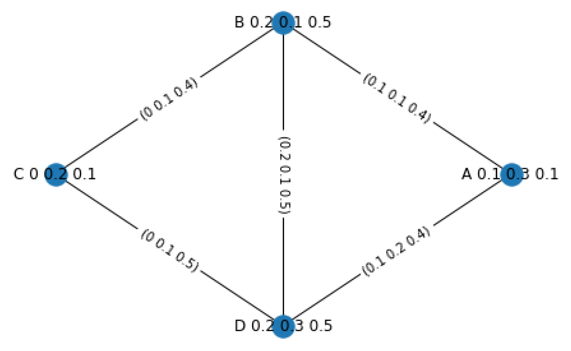
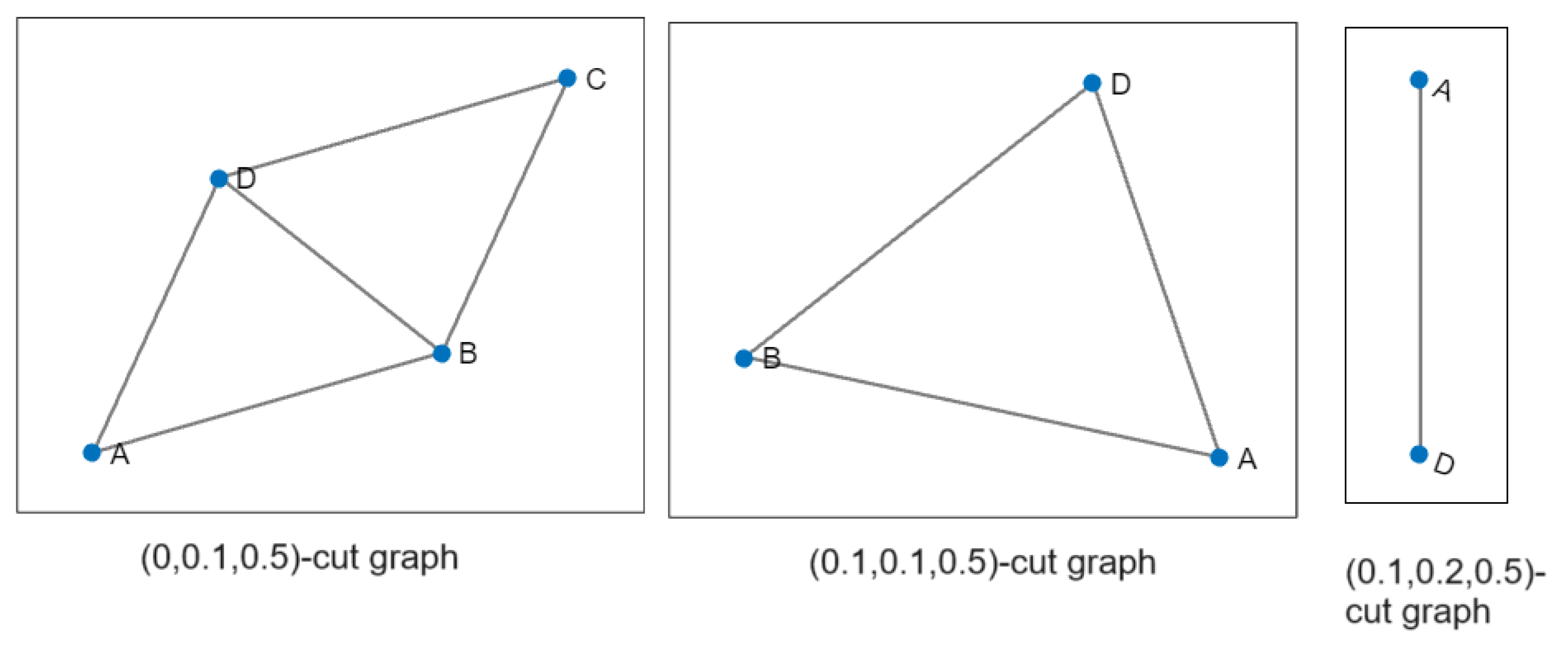
Example 1. Let us consider PFG in Figure 1. The set is a PFVS on universal set . - 1.
The pairs of strongly adjacent vertices are and . Meanwhile, is the pair of weakly adjacent vertices.
- 2.
Therefore, we obtain the PF-subset . Since B and D are strongly adjacent, , and . We obtain the family .
- 3.
Thus, the chromatic number of is .
Figure 1.
The picture fuzzy graph for Example 1.
Figure 1.
The picture fuzzy graph for Example 1.
3.3. The Chromatic Number of PFGs Based on -Cut Coloring
In this part, we discuss the concept of -cut of PFGs and the cut chromatic number in Definition 12.
Definition 12 ([
31])
. Given a PFG and its underlying graph , a level set of is defined as a set , whereas a level set of is set . Moreover, a level set of is a set . Given , an -cut of is a crisp graph whereandThe -cut chromatic number, denoted by , is the chromatic number obtained from crisp coloring of the cut . Example 2. We present an illustration of Definition 12 for PFG in Figure 1. The level set of and are , and , respectively. Meanwhile, the level set of is . Examples of (0, 0.1, 0.5)-cut, (0.1, 0.1, 0.5)-cut, and (0.1, 0.2, 0.5)-cut are depicted in Figure 2. The (0, 0.1, 0.5)-cut chromatic number is 3, the (0.1, 0.1, 0.5)-cut chromatic number is also 3, and the (0.1, 0.2, 0.5)-cut chromatic number is 2. 4. Main Results
In this section, we present some properties of the chromatic number of PFGs and an algorithm to compute the chromatic number.
4.1. Some Characteristics of the Chromatic Number of PFGs
In this part, we investigate an upper bound for the chromatic number of PFGs in Theorem 3.
Theorem 3. If is a PFG with the underlying graph , then Proof. Let Assume is a family of PF-subsets on where , , .
Suppose that
Based on Conditions 1–2 in Definition 11, we have:
When every pair of vertices is strongly adjacent, the vertices should be placed in different picture fuzzy (PF) subsets. According to the Condition 3 in Definition 11, we have n PF subsets . Meanwhile, . Thus, . Otherwise, when there is a pair or weakly adjacent vertices, . It is a contradiction. Thus, □
Moreover, we investigate the connection between the chromatic number of PFGs based on strong and weak adjacencies and the -cut chromatic number in Definition 12. Firstly, we define the chromatic number of a PFG by means of its-cut chromatic number.
Definition 13. Let be a PFG. The chromatic number of through the -cut chromatic number is defined as follows:where L is the level set of and . When , Definition 13 becomes the chromatic number of IFGs. In certain conditions, we prove that the chromatic number of the underlying graph of PFG is equal to the chromatic number concept in Definition 13.
Example 3. Let us consider Example 2. According to Definition 13, the chromatic number of through the -cut is Theorem 4. Given a PFG with the underlying graph If , and then the chromatic number of : Proof. Since , and we have
Further, all vertices and edges of become elements of the crisp graph . This implies and □
Theorem 5. Let be a PFG with the underlying graph If all edges in connect strongly adjacent vertices, then Proof. Assume that . According to Definition 11, we have a family of PF-subsets of such that it satisfies 3 conditions in Definition 11:
,
, for .
Based on the third condition in Definition 11, we have where , , and (since all edges in connect strongly adjacent vertices). This shows that each becomes a crisp independent vertex set in for .
Hence, the family becomes a partition of into k-independent vertex set (crisp set). Therefore, □
According to Theorem 5, we obtain the following corollary.
Corollary 2. If is a complete picture fuzzy graph (CPFG) with n vertices, then .
4.2. An Algorithm for Finding the Chromatic Number of PFGs
We create an algorithm to compute the chromatic number of PFGs with the exception for CPFG. We use the assumption that not all edges in connect strongly adjacent vertices.
Algorithm 1 can also be used for the coloring of IFGs when the inputs are the intuitionistic fuzzy vertex set and the intuitionistic fuzzy edge set.
| Algorithm 1 To find the chromatic number of PFGs |
- Input:
The PFG with the elements:
Vertex set , , and edge set . Degree of vertices , with . Degree of edges , where
- Output:
The chromatic number: - 1:
for h = 1 to n − 1 do - 2:
for j = 1 to n − h do - 3:
Check for all pairs - 4:
if and then - 5:
“ and are strongly adjacent” - 6:
else - 7:
“ and are weakly adjacent” - 8:
Assign for - 9:
end if - 10:
end for - 11:
end for - 12:
if All pairs in are strongly adjacent vertices then - 13:
- 14:
if then - 15:
Create two picture fuzzy (PF) subsets and get . - 16:
end if - 17:
else - 18:
Go to Step 20 - 19:
end if - 20:
if
then - 21:
Initialization - 22:
sc1 = number of elements of - 23:
for i = 1 to sc1-1 do - 24:
if then - 25:
Assign - 26:
end if - 27:
end for - 28:
if elements of are not elements of then - 29:
Assign - 30:
else - 31:
- 32:
end if - 33:
Repeat the process in Steps 28–32 to create the picture fuzzy (PF) subsets such that , for , and every pair of strongly adjacent vertices belongs to different for - 34:
if There is only one PF subset then - 35:
Stop the process, and go to Step 47 - 36:
end if - 37:
else - 38:
Initialization - 39:
Do the same process in Steps 22–33 to get the PF-subsets - 40:
end if - 41:
Do the same process in Steps 21–33 to get the PF subsets with initialization and . - 42:
if
then - 43:
Stop the process, and go to Step 47 - 44:
else - 45:
Back to Step 41 - 46:
end if - 47:
Choose and obtain the family where . - 48:
Obtain the chromatic number: .
|
We show that Algorithm 1 gives the chromatic number for and proves the correctness of the algorithm by using mathematical induction on the cardinality as follows.
Base step: for and .
If the two vertices in V are strongly adjacent vertices, then Steps 1–11 will produce . Further, Steps 12–16 give , and the chromatic number . If the two vertices in V are weakly adjacent vertices, then Steps 1–11 produce Further, Steps 17–36 give PF-subset Finally, Steps 47–48 give the family and . Thus, the chromatic number The base step is satisfied.
Inductive step: Assume that Algorithm 1 is correct for cardinality
. Steps 1–11 produce the set of weakly adjacent vertices and the set of strongly adjacent vertices. Furthermore, Steps 20–41 give the PF-subsets:
In Steps 42–48, we obtain
, where
and
. The chromatic number
.
We prove that Algorithm 1 is correct for PFG with cardinality .
Assume that there is an edge . Based on the assumption in the inductive step, we have the family . Without a loss of generality, vertex is an element of the PF subset
If is a pair of weakly adjacent vertices, then vertex could be an element of Otherwise, when is a pair of strongly adjacent vertices, vertex could be an element of , or , or ⋯, , and hence we obtain the chromatic number According to Theorem 3, the chromatic number . Thus, the inductive step is true and Algorithm 1 is correct.
Examples 4 and 5 show the determination of the chromatic number of PFGs by employing Algorithm 1, and the performance of the algorithm is evaluated using Python and Matlab R2022b.
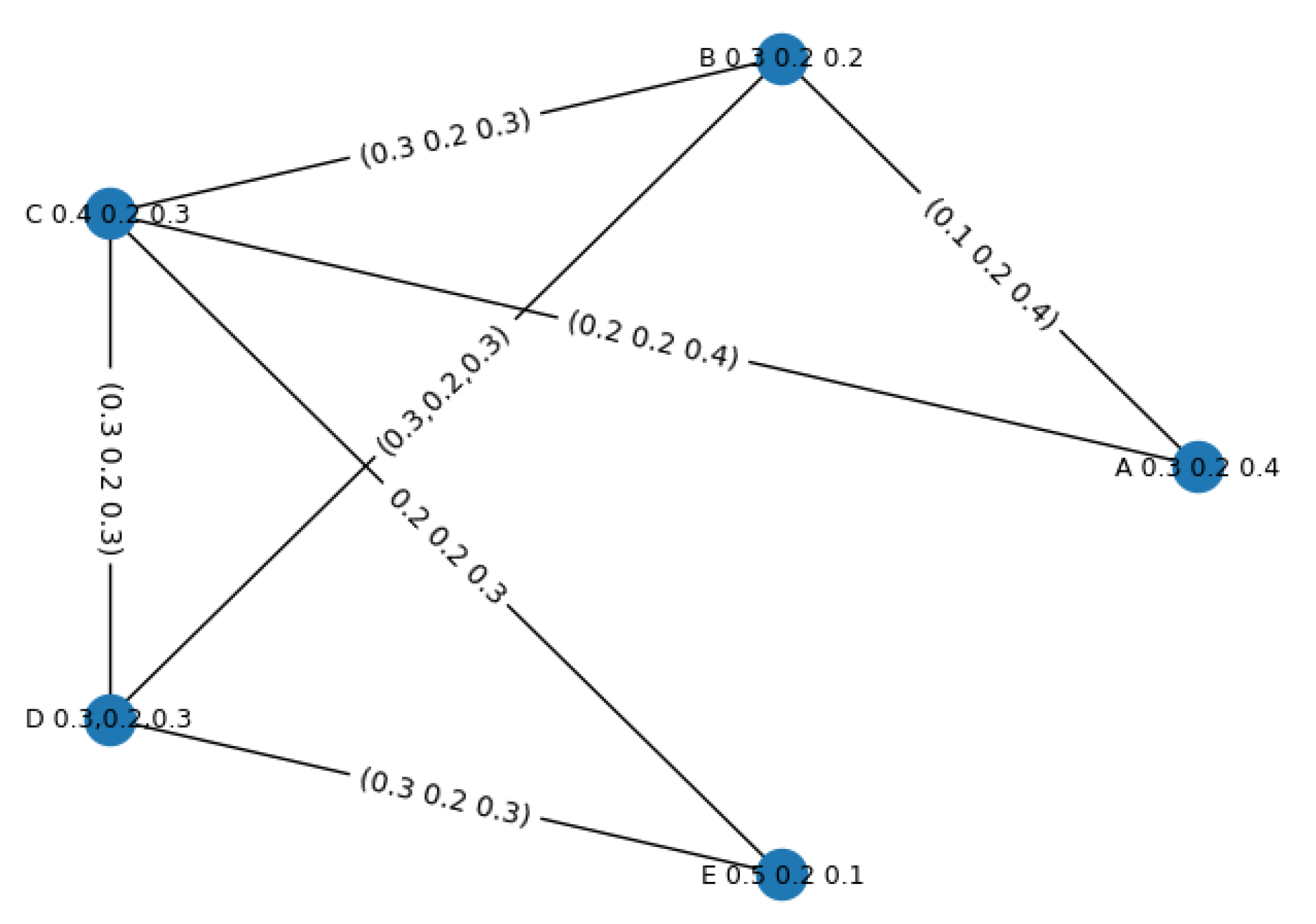
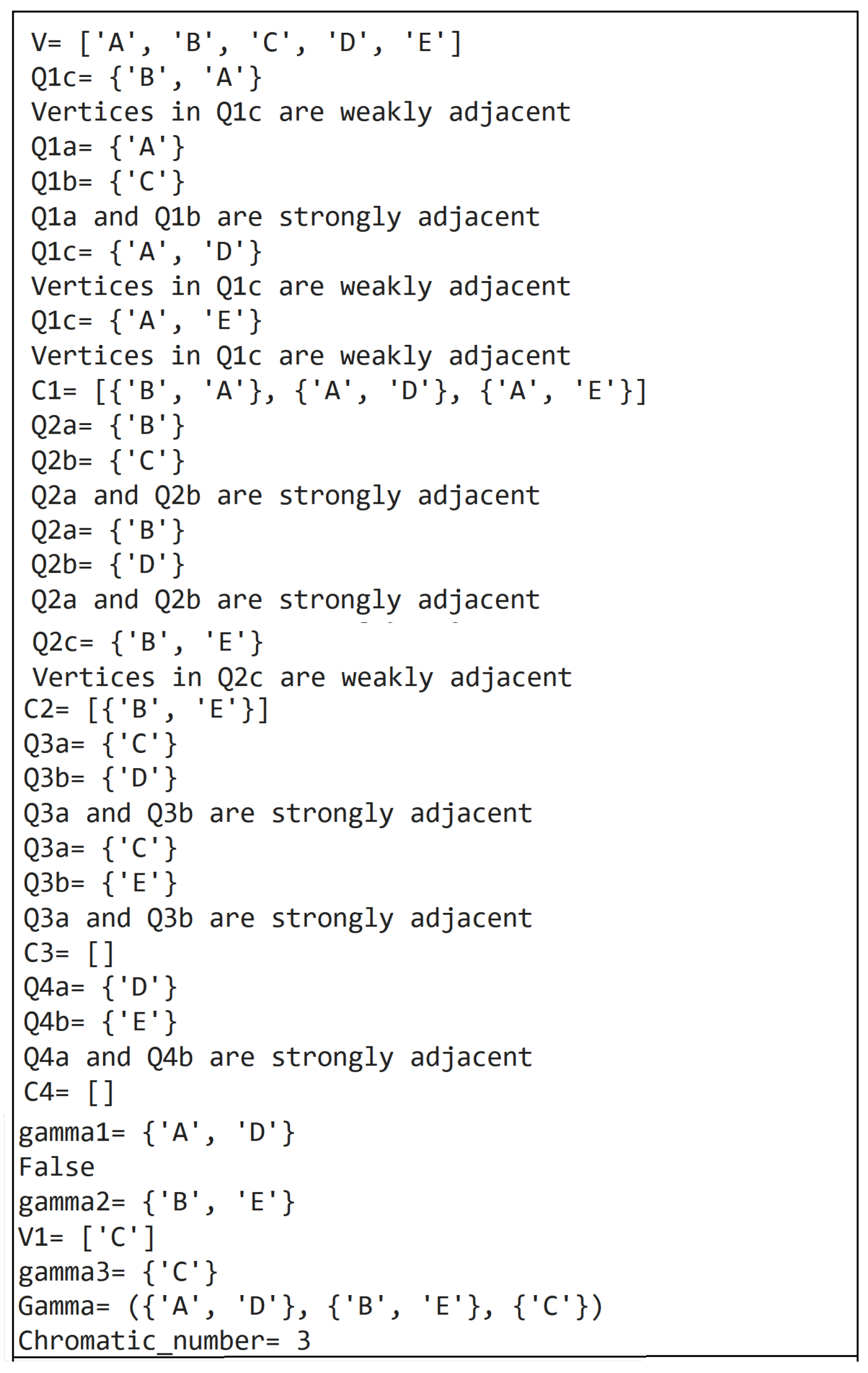
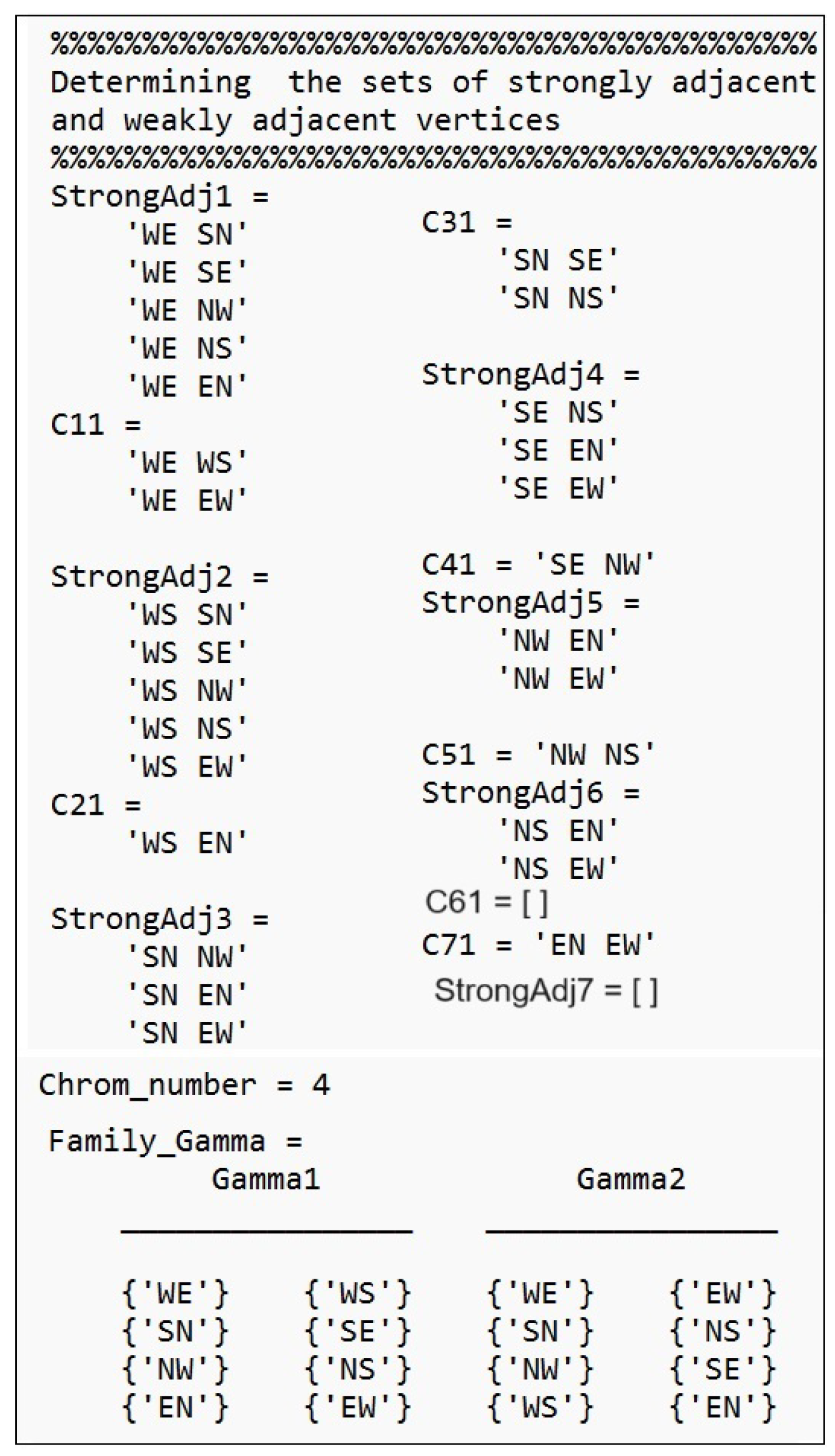
Example 4. Given PFG in Figure 3 with picture fuzzy vertex set and picture fuzzy edge set . The output of Algorithm 1 in determining the chromatic number of is presented in Figure 4. - 1.
In Steps 1–11, we obtain the sets of the pairs of weakly adjacent vertices, i.e., .
- 2.
In Steps 17–41, we obtain the PF-subsets with the initialization .
Other PF-subsets are as follows:
, , and , with the initialization .
- 3.
In Steps 42–48, since then stop. We choose and obtain the family . Thus, the chromatic number .
Figure 3.
The picture fuzzy graph for Example 4.
Figure 3.
The picture fuzzy graph for Example 4.
Figure 4.
The output of Algorithm 1 for finding
in
Figure 3.
Figure 4.
The output of Algorithm 1 for finding
in
Figure 3.
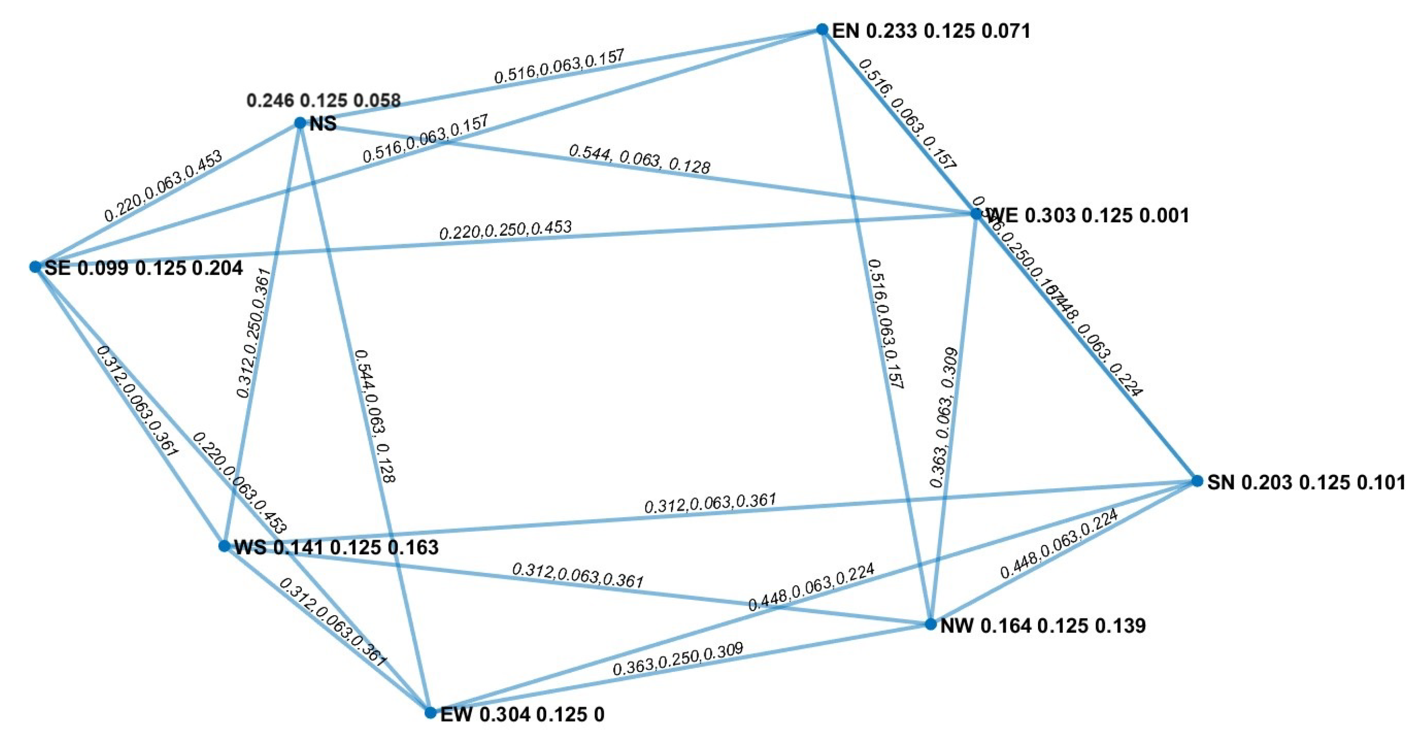
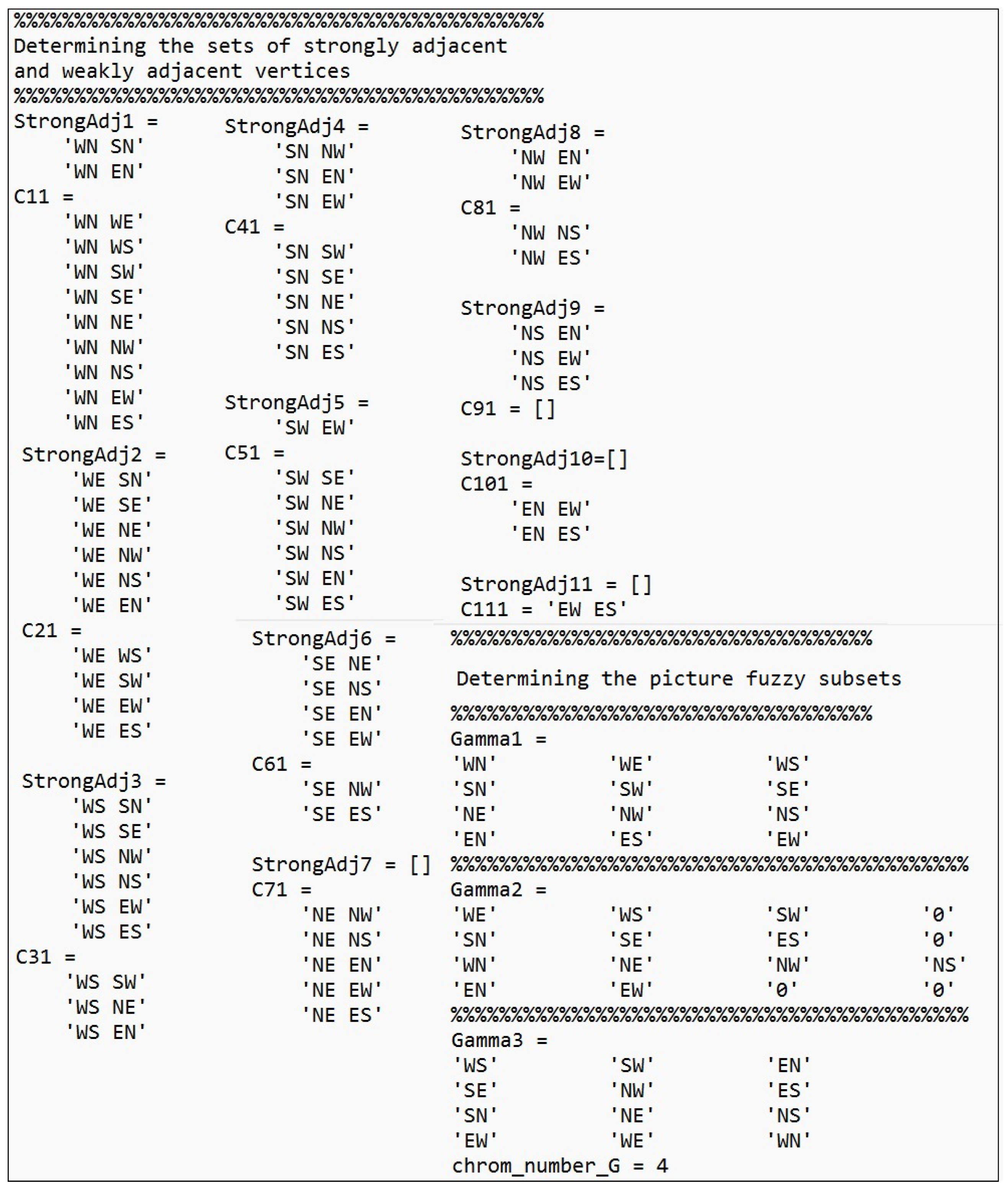
Example 5. Let us consider PFG in Figure 5, where is a PFS on The output of Algorithm 1 for PFG in Figure 5 is shown in Figure 6. We obtain the family and the chromatic number .
Figure 5.
The PFG for Example 5.
Figure 5.
The PFG for Example 5.
Figure 6.
The output of Algorithm 1 for finding
in
Figure 5.
Figure 6.
The output of Algorithm 1 for finding
in
Figure 5.
5. Experimental Result
In this section, we discuss an implementation of Algorithm 1 in determining traffic signal phasing at an intersection. A phase is defined as any traffic light display that has its own timings, and it determines how a specific vehicle or pedestrian will move, whereas the term phase set refers to “any distinct combination of concurrent vehicle or pedestrian phases”. Conflicting phases are those that cannot both have green indicators at the same time [
39]. There are two types of conflicts between traffic movements at an intersection. The first type is crossing conflict, which is a collision that occurs when two separate directions of traffic try to cross paths at one spot. The second type is merging conflict, i.e., a conflict that happens when vehicles from multiple lanes or directions merge into a single lane traveling in a single direction [
40].
Traffic flow is “the number of traffic elements passing an undisturbed point upstream in the approach per unit of time”. It is measured by the number of vehicles per hour or the passenger car unit (pcu) per hour [
40]. In this research, the traffic flow data are presented in pcu per hour, where the conversion factors are as follows: 0.2 for motor cycle (MC); 1 for light vehicle (LV), including “passenger cars, pick-up, and micro buses”; and 1.3 for heavy vehicle (HV), including “two or three-axle trucks and buses”.
5.1. The Method to Model Traffic Flows at an Intersection Using PFGs
We visualize traffic movements from different directions as vertices and connect two vertices with an edge if the two movements are in conflict (crossing conflict or merging conflict). Hence, we obtain the data of vertex and edge sets V and E, respectively. The degrees of edges and vertices show the following circumstances:
A vertex’s membership degree () indicates the possibility of the crowdedness of traffic flow on the movement x at the intersection. A vertex’s non-membership degree () shows whether the flow of traffic on the movement x is likely to be free of congestion. The NeuM degree of a vertex () indicates the possibility of an unknown circumstance about the crowdedness of traffic flow on x. We obtain a PFVS .
Traffic flow on an edge that connects two vertices (traffic movements) is determined through the minimum of traffic flows on both movements. In addition, the membership degree of any edge in , that is, , indicates the possibility of the crowdedness of traffic flows on conflicting movements . On the contrary, the non-membership degree shows the possibility of the non-crowdedness of traffic flows on . The NeuM degree represents the possibility of the unknown condition of the crowdedness of traffic flows on . We obtain a PFES .
The degrees of vertices and edges are determined as follows:
The membership degree
is calculated through triangular or trapezoidal membership functions, whereas the non-membership degree is calculated through Equation (
1) in Corollary 1, i.e.,
and
by choosing
where
stands for traffic flow on movement
x.
The NeuM degree
is determined through the function
g in Theorem 2:
where
for
and
([
35]). The NeuM degree of each edge
is defined similarly.
The membership degree and non-membership degree are calculated through formulas in Corollary 1: , where
,
by choosing
5.2. Case Study
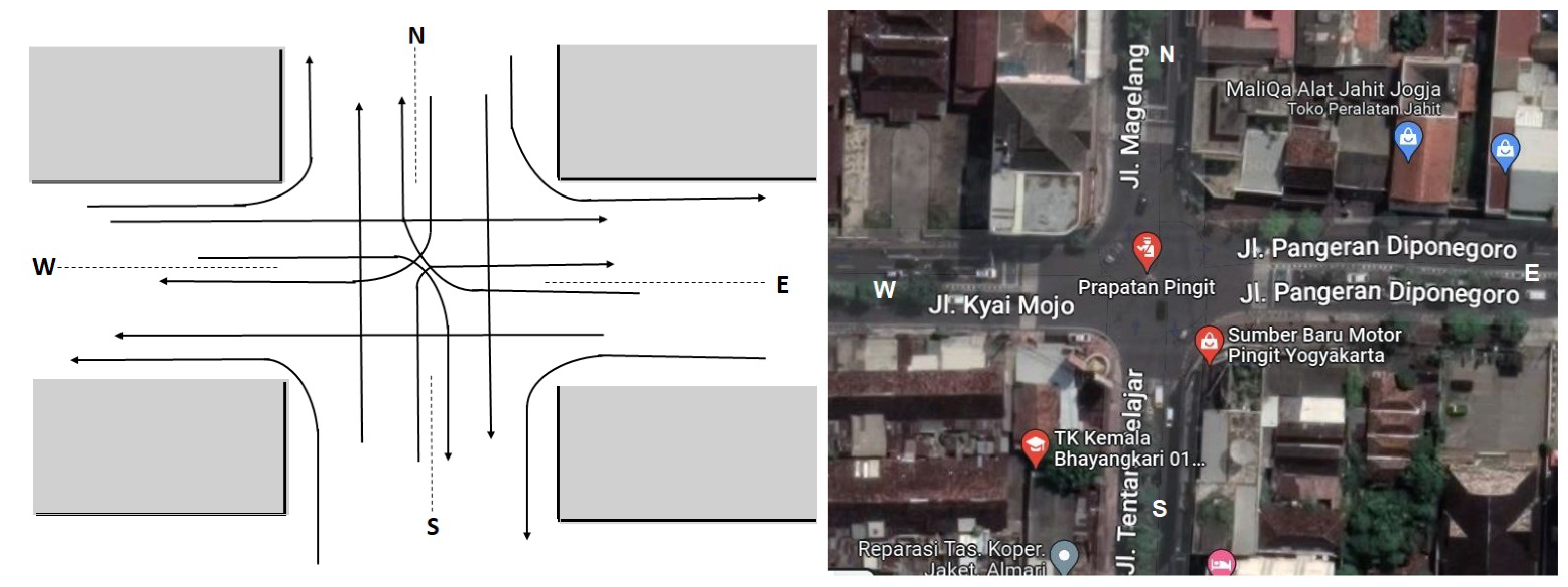
We take a case study at an intersection in the Special Region of Yogyakarta, Indonesia, i.e., the Pingit intersection. The location of the intersection is depicted in
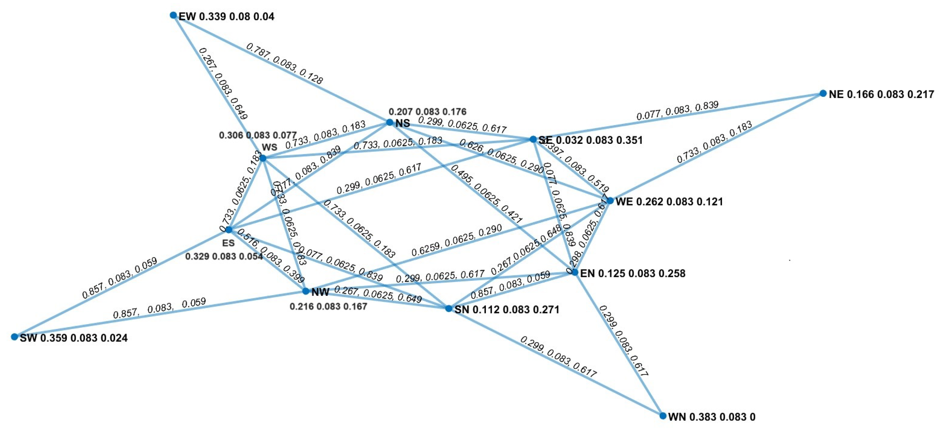
Figure 7 (right side). Tentara Pelajar street is in the Southern (S) direction, Diponegoro street is to the Eastern (E) direction, Magelang street is to the Northern (N) direction, and Kyai Mojo street is to the Western (W) direction.
A sketch of the intersection is also given in
Figure 7 (left side). We collect the data of traffic flows on 25–27 January 2023 in the morning (06.30–07.30 a.m.) and in the evening (16.30–17.30 p.m.). There are 12 traffic movements in the intersection, i.e., WN, WE, WS, SN, SW, SE, NE, NW, NS, EN, EW, and ES. This means that the vertex set
V contains 12 vertices.
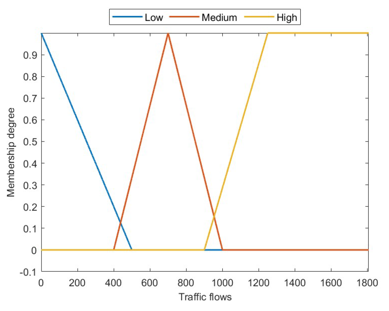
The next step is to transform the traffic flow data into PFVS
, wherein the membership degree of each element is determined via triangular and trapezoidal membership functions in
Figure 8.
The PFVS
of traffic flows in the intersection is displayed in
Table 1.
It is shown in
Table 1 that traffic flows on WN and EW have a high possibility of being crowded compared to traffic flows on other movements. Conversely, the traffic flow on SW has a lower possibility of being crowded.
Further, the picture fuzzy edge sets from crossing and merging conflicts in the Pingit intersection are shown in
Table 2 and
Table 3, respectively. We observe that most of the edges in both tables connect strongly adjacent vertices. Moreover, the traffic flows on edges WS SN, WS SE, WS NW, WS EW, SW NW, SW and EW have a high possibility of being crowded.
The PFG model
of traffic flow data is depicted in
Figure 9.
We obtain the chromatic number
through Algorithm 1, and it has been evaluated in Matlab R2022b, where the output is depicted in
Figure 10. The traffic flows can be arranged in 4 phases, and the patterns of traffic signal phasing are presented in
Table 4.
5.3. Comparison to the Fuzzy Graph Coloring Method
In this part, we compare the result in
Table 4 with a traffic signal phasing obtained from the fuzzy graph coloring method based on
-fuzzy independent vertices (
) as given in [
33]. The fuzzy graph model of traffic flows in the Pingit intersection is depicted in
Figure 11.
For
, the sets
,
, and
are the sets of
-fuzzy independent vertices since
for each pair
in the above sets. Therefore, we obtain 4-phase scheduling as follows:
We observe that some pairs of vertices in (
2) are elements of merging conflict in
Table 3. Hence, the traffic signal phasing obtained from PFG coloring in
Table 4 is safer than the signal phasing from the fuzzy graph coloring in (
2) since there are no traffic flows from merging conflict that move simultaneously at the same phase.
6. Conclusions
The concept of strong and weak adjacencies between vertices could be implemented in making decisions regarding real-world problems. Therefore, we generalized the concept from the intuitionistic fuzzy graph (IFG) into the picture fuzzy graph (PFG) in the previous work. In this research, we investigated some of the characteristics of the chromatic number of PFGs based on strong and weak adjacencies between vertices and their relation to the -cut chromatic numbers. Furthermore, we constructed an algorithm (Algorithm 1) for determining the chromatic number of PFGs and implement it in Python and Matlab R2022b to assess the algorithm’s performance. The correctness of Algorithm 1 was also proved using mathematical induction.
Additionally, we improved the method to model traffic flows at an intersection using PFGs and to determine an intersection’s traffic light phasing. We took a case study at an intersection in the Special Region of Yogyakarta-Indonesia to evaluate the method. The outcome demonstrated that there were no concurrent traffic flows from merging conflict that moved at the same phase. The traffic signal phasing acquired using the PFG coloring method was found to be safer than the signal phasing obtained using the fuzzy graph coloring method.
Further research can be carried out to improve the method for handling traffic signal phasing at any intersection, such as implementing the method for the five way-intersection and integrating the algorithm with automatic counting for traffic flow data at the intersection. In the basic theories of PFG’s coloring, we can investigate the chromatic number of certain operations of two PFGs, such as union, join, Cartesian product, and composition of two PFGs.


