Article

Measuring the Performance of Ant Colony Optimization Algorithms for the Dynamic Traveling Salesman Problem

by
Michalis Mavrovouniotis
1,2,*,
Maria N. Anastasiadou
1 and
Diofantos Hadjimitsis
1,2
1
ERATOSTHENES Centre of Excellence, 3012 Limassol, Cyprus
2
Department of Civil Engineering and Geomatics, Cyprus University of Technology, 3036 Limassol, Cyprus
*
Author to whom correspondence should be addressed.
Algorithms 2023, 16(12), 545; https://doi.org/10.3390/a16120545
Submission received: 24 October 2023 / Revised: 23 November 2023 / Accepted: 25 November 2023 / Published: 28 November 2023

Abstract

:
Ant colony optimization (ACO) has proven its adaptation capabilities on optimization problems with dynamic environments. In this work, the dynamic traveling salesman problem (DTSP) is used as the base problem to generate dynamic test cases. Two types of dynamic changes for the DTSP are considered: (1) node changes and (2) weight changes. In the experiments, ACO algorithms are systematically compared in different DTSP test cases. Statistical tests are performed using the arithmetic mean and standard deviation of ACO algorithms, which is the standard method of comparing ACO algorithms. To complement the comparisons, the quantiles of the distribution are also used to measure the peak-, average-, and bad-case performance of ACO algorithms. The experimental results demonstrate some advantages of using quantiles for evaluating the performance of ACO algorithms in some DTSP test cases.

1. Introduction

Ant colony optimization (ACO) is a mainstream swarm intelligence algorithm inspired by the foraging behavior of real ant colonies [1,2,3]. In ACO, a colony of artificial ants constructs solutions guided by artificial pheromone trails and some heuristic information. ACO has been successfully applied in various complex optimization problems [4,5,6]. However, in most real-world applications, the optimization problem has a dynamic environment [7]. In particular, the  environment of the optimization problem, including objective function, constraints, search space, input variables, and so on, may change over time.
Major challenges occur when addressing dynamic optimization problems because repeated optimization of the changing optimum is required. The optimal solution in which the algorithm has converged to it before the dynamic change may not be the optimal solution after the dynamic change. Consequently, the optimization process needs to be restarted in order to search for a new optimal solution. However, it may not be very efficient to restart the optimization process from scratch in complex problems (e.g., NP -hard combinatorial problems), as they require huge computational efforts and time [8].
A more efficient way to address dynamic optimization problems is to use knowledge from previously optimized environments to speed up the re-optimization process [9]. With ACO algorithms, this knowledge can be transferred via the pheromone trails generated in the previous environments. However, the pheromone trails of the previous environment may contain information directing the search process to the previous optimal solution, which may represent a poor local optimum in the current environment [10]. Several strategies have been integrated to enhance the adaptation capabilities of ACO in dynamic optimization problems, such as the generation of new ants using immigrant schemes [11,12], population-based pheromone update strategies [13], multiple ant colonies [14], and memetic computing [15].
In this work, the traveling salesman problem (TSP) is used as the base optimization problem to generate dynamic test cases using the benchmark generator proposed in [10]. A conventional ACO [16] and a population-based ACO [13] that use pheromone evaporation and memory archive, respectively, to adapt to dynamic changes are applied to the generated dynamic TSP (DTSP) test cases.
The most common method to evaluate the performance of ACO in dynamic environments is used in the experiments, that is, to  obtain the mean and standard deviation (for multiple independent executions) for the generated DTSPs. Statistical tests are performed to compare the algorithms. In [17], it is argued that, for stochastic algorithms (e.g., ACO algorithms), this way of comparison may not be very informative. This is because the distribution of executing ACO algorithms multiple times may be asymmetrical and, hence, outlier values may affect the mean value. Consequently, inadequate information regarding the average performance of the algorithms may be provided. In contrast, quantiles of the distribution may address this issue with the use of median values as an average performance measurement.
The rest of the paper is structured as follows. Section 2 provides a description of the TSP as well as a description of the generation of dynamic test cases. Section 3 describes the application of the ACO metaheuristic to the TSP. In addition, the pheromone update policies in dynamic environments for the two ACO algorithms used in the experiments are described. Section 4 presents the experimental setup and results. An analysis of the obtained results is provided. Section 5 concludes this work.

2. The Dynamic Traveling Salesman Problem

2.1. Problem Definition

The TSP is a well-known combinatorial optimization problem proven to be NP -hard [18]. The problem can be described as follows: a salesperson must visit multiple cities once and only once, starting from one city and returning finally, to the same city [19]. Typically, a fully connected weighted graph G = ( N , A ) is used to model the TSP, where N = { 1 , , n } is the set of n cities and A = { ( i , j ) N : i j } is a set of arcs connecting these cities. Each arc ( i , j ) is associated with a non-negative value d i j , which is the distance between cities i and j.
The TSP solution s = [ 1 , , n ] is a permutation of city indices, and the objective function of the TSP is defined as follows:
ϕ ( s ) = i = 1 n 1 d s ( i ) s ( i + 1 ) + d s ( n ) s ( 1 ) .

2.2. Generating Dynamic Environments

There are two main dynamic versions of the TSP in which: (a) the values associated with the arcs are changing [12,20,21,22]; and (b) the cities to be visited are changing [11,13,23]. The dynamic benchmark generator (Available at https://github.com/Mavrovouniotis/ACODTSP (accessed on 23 February 2023)) used in [10] is adopted to generate DTSP test cases. Each DTSP test case is characterized by the type of change (either the weights or the nodes change), the magnitude of change (either small, medium, or severe), and the frequency of change (either fast or slow).
For the DTSP with weight changes, a factor that increases or decreases the value of arcs connecting cities i and j is assigned every environmental period T, i.e.,  d i j ( T ) , where T = t / f , f is the frequency of a dynamic change, and t is the algorithmic iteration count. The value of the arc ( i , j ) changes as follows:
d i j ( T + 1 ) = d i j ( 0 ) + R i j , i f   a r c ( i , j ) A r n d ( T ) , d i j ( T ) , o t h e r w i s e ,
where R i j is a random number drawn from a normal distribution with a zero mean and standard deviation proportional to the initial value of the arc d i j ( 0 ) , A r n d ( T ) A is a set of randomly selected arcs with size m n ( n 1 ) in which their values are subject to change at environmental period index T, and  m ( 0 , 1 ) is the magnitude of change. Therefore, the quality value of solution s for the DTSP depends on the parameter t and, thus, is evaluated as ϕ ( s , t ) . In other words, the  quality of a solution s at time t may be different at time t + 1 .
For the DTSP with node changes, a newly generated set of cities, i.e., N r n d ( T ) , is initialized, with n random cities in the range of the actual set of cities N. A dynamic change is generated for every f function evaluation, in which exactly m n cities are randomly chosen from N r n d ( T ) to replace exactly m n randomly chosen cities from N, where f and m define the frequency and magnitude of a dynamic change, respectively, as above.

3. Addressing the Dynamic Traveling Salesman Problem

3.1. Ant Colony Optimization Metaheuristic

ACO has been designed for graph problems and, thus, it can be applied directly to the TSP, which is modeled as a weighted graph [24,25,26]. All arcs are associated with a pheromone trail value τ i j and some heuristic information value η i j . Initially, the pheromone trails are assigned with equal values, i.e.,  τ i j τ 0 , A , where τ 0 is the initial pheromone value. The heuristic information at environment T is defined as η i j = 1 / d i j ( T ) . A colony of ω artificial ants is initially positioned in different randomly selected cities. Each ant k will select the next city to visit based on the existing pheromone trails τ i j and the defined heuristic information η i j of arc ( i , j ) . Each ant will visit all cities once, in order to represent a feasible DTSP solution. Then, the pheromone trails associated with the ω solutions constructed by the ants will be reinforced according to their quality value.

3.1.1. Constructing Solutions

With a probability ( 1 q 0 ) , where 0 q 0 1 is a parameter of the decision rule, the k-th chooses the next city j from city i, from a probability distribution that is defined as follows:
p i j k = τ i j α η i j β l N i k τ i l α η i l β , i f j N i k , 0 , o t h e r w i s e
where τ i j and η i j are the existing pheromone trail and heuristic information values, respectively, N i k is the set of cities that ant k has not visited yet, and α and β are the two parameters that determine the relative influence of the pheromone trail and heuristic information, respectively. With  probability q 0 , ant k chooses the next city, i.e., j, with  the maximum probability as follows [27]:
j = argmax j N i k τ i j α η i j β .
This selection process will continue until each ant has visited all cities once and only once, as shown in Algorithm 1. The constructed solutions will be evaluated based on Equation (3).

3.1.2. Updating Pheromone Trails

The pheromone update procedure consists of two parts: (1) pheromone evaporation, in which all pheromone trails are reduced by a constant rate; and (2) pheromone deposit, in which ants increase the pheromone trails associated with their constructed solutions.
In this work, the pheromone policy of the MAX MIN Ant System ( MM AS) algorithm is used, which is one of the best-performing ACO variants [28,29]. Firstly, in the pheromone update procedure of MM AS, an evaporation is performed on all pheromone trails as follows:
τ i j 1 ρ τ i j , ( i , j ) A ,
Algorithm 1 Construct Solutions (t)
  1:
for each ant k do
  2:
    s k
  3:
    r random { 1 , , n }
  4:
    s k s k r
  5:
   while  s k length not equal with n do
  6:
      j select next city N i k
  7:
      s k s k j
  8:
   end while
  9:
    C k ϕ ( s k , t )
10:
end for
where 0 < ρ 1 is the rate of evaporation.
Thereafter, the best ant is allowed to deposit pheromone as follows:
τ i j τ i j + Δ τ i j b e s t , ( i , j ) s b e s t ,
where s b e s t is the solution generated by the best ant and Δ τ i j b e s t = 1 / C b e s t , where C b e s t = ϕ ( s b e s t , t ) is the quality value of DTSP solution s b e s t . The best ant to deposit pheromone may be either the best-so-far ant, in which case Δ τ i j b e s t = 1 / C b s , where C b s = ϕ ( s b s , t ) is the solution quality of the best-so-far ant, or the iteration-best ant, in which case Δ τ i j b e s t = 1 / C i b , where C i b = ϕ ( s i b , t ) is the solution quality of the best ant of the iteration. By default, the iteration-best ant is used to update the pheromone trails and, occasionally, the best-so-far ant. The pheromone trail values in MM AS are kept to the interval [ τ m i n , τ m a x ] , where τ m i n and τ m a x are the minimum and maximum pheromone trails limits, respectively. The overall MM AS pheromone update is presented in Algorithm 2, lines 1–20.

3.2. Adapting in Dynamic Environments

ACO algorithms have proven effective in addressing dynamic optimization problems because they are very robust algorithms, according to Bonabeau et al. [30]. However, when a dynamic change occurs, the ACO’s pheromone trails of the previous environment will become outdated because they will be associated with the previous optimum. A straightforward way to tackle the dynamic changes in the DTSP using a conventional ACO, such as the MM AS, is to restart the optimization process whenever changes occur. In particular, the pheromone trail limit values τ m a x and τ m i n are reset back to their initial values, and all the pheromone trails are re-initialized to the initial τ 0 value, as in Equation (5), whenever a dynamic change is detected.
There are two concerns when restarting an ACO: (1) the dynamic changes are not always detectable [31], and (2) a portion of the previous pheromone trails that can help discover the new optimum faster is erased [32]. For the first concern, the changes in the DTSP can be detected by re-evaluating a constant solution (or detector) on every iteration (note that more than one detector can be used). If a change occurs in the quality of the detector, then a dynamic change is recorded. In this way, a change is always detected for the DTSP with node changes but not for the DTSP with weight changes. This is because the weights affected by the dynamic change may not belong to that particular detector, and hence, its quality will not be affected [10]. For the second concern, the pheromone trails of the previous environment will be most probably useful when the changing environments are correlated, e.g.,  when the dynamic changes are small to medium, the new environment is more likely to be similar to the previous environment. As a consequence, some of the previous pheromone trails will still be useful to the new environment.
Algorithm 2 Pheromone Update  ( t , s i b , s b s )
  1:
if MM AS is selected then
  2:
    τ m a x 1 / ρ C b s
  3:
    τ m i n τ m a x 1 0.05 n / c a n d 1 · 0.05 n
  4:
   for  ( i , j ) A do
  5:
      τ i j ( 1 ρ ) τ i j
  6:
   end for
  7:
    s b e s t s i b | | s b s
  8:
    Δ τ i j b e s t 1 / C i b | | 1 / C b s
  9:
   for each arc ( i , j ) s b e s t do
10:
      τ i j τ i j + Δ τ i j b e s t
11:
   end for
12:
   for  ( i , j ) A do
13:
     if  τ i j > τ m a x then
14:
         τ i j τ m a x
15:
     end if
16:
     if  τ i j < τ m i n then
17:
         τ i j τ m i n
18:
     end if
19:
   end for
20:
end if
21:
if P-ACO is selected then
22:
    Δ τ ( τ m a x τ 0 ) / K
23:
   if  t = = K then
24:
      p o p ( t ) p o p ( t ) s r
25:
     for each arc ( i , j ) s r do
26:
         τ i j τ i j Δ τ
27:
     end for
28:
   end if
29:
    p o p ( t ) p o p ( t ) s i b
30:
   for each arc ( i , j ) s i b do
31:
      τ i j τ i j + Δ τ
32:
   end for
33:
end if
Therefore, a more efficient way is to allow the pheromone evaporation defined in Equation (5) to remove the useless pheromone trails and utilize the useful pheromone trails of the previous environment. Specifically, the useless pheromone trails will reach the τ m i n value due to the constant deduction of pheromone evaporation, whereas the useful pheromone trails will be reinforced up to the τ m a x due to the pheromone deposit in Equation (6). In other words, ACO will be able to adapt to the newly generated environment.
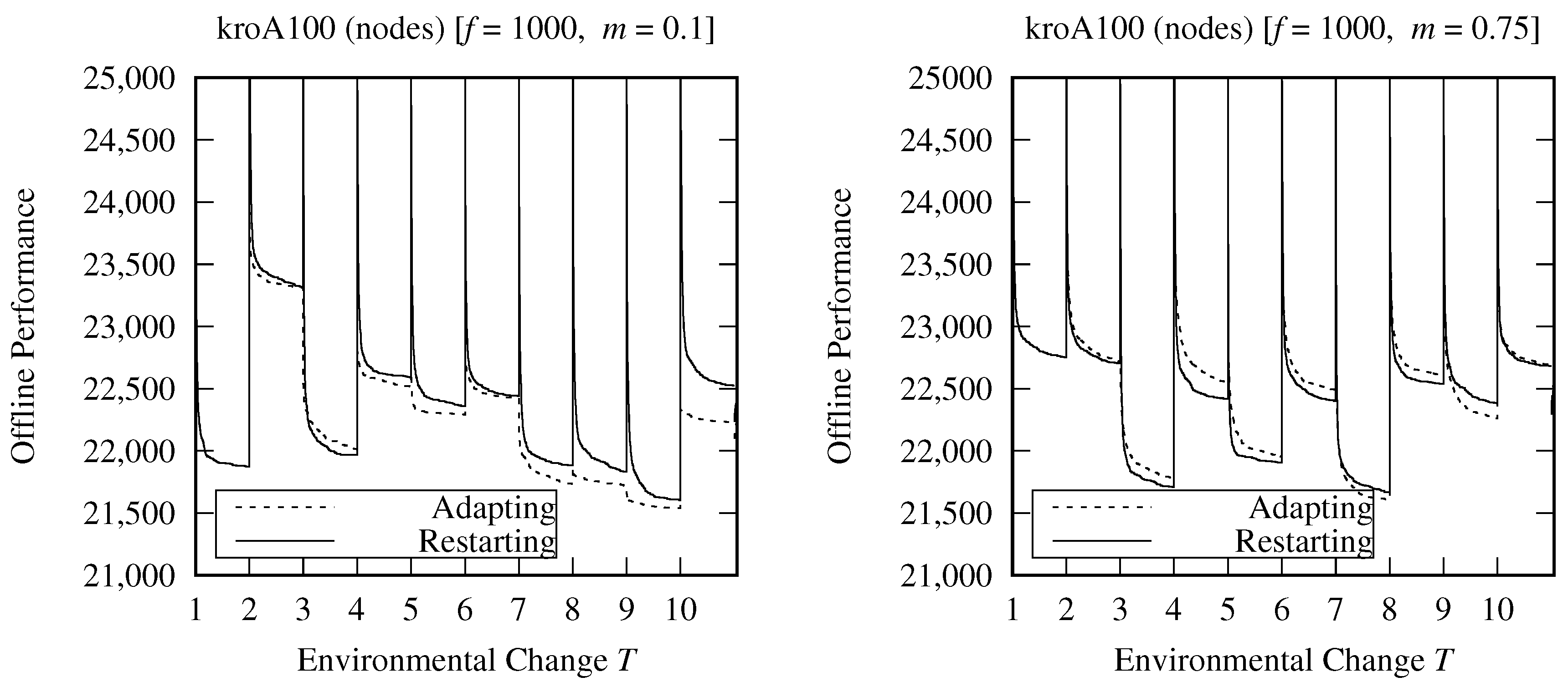
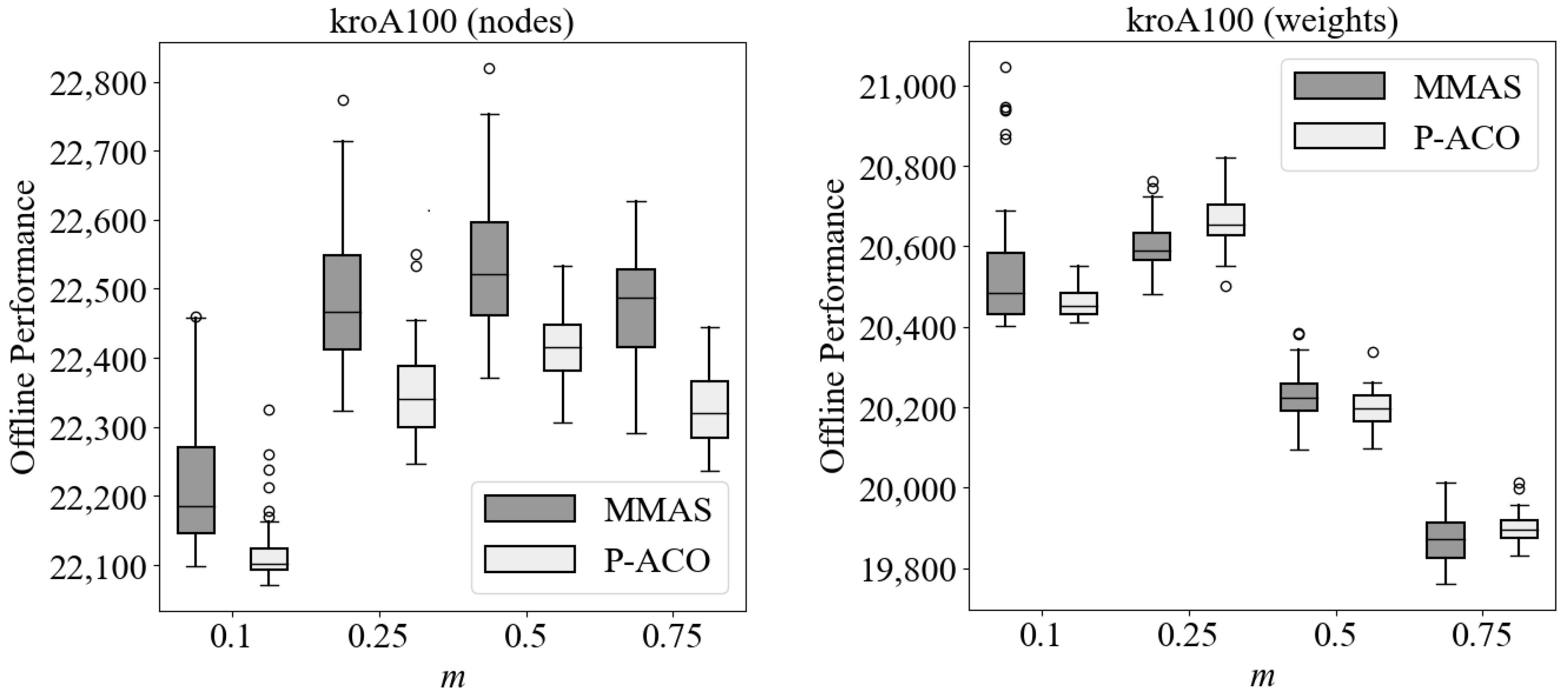
Figure 1 demonstrates the performance of MM AS with and without pheromone re-initialization and proves our claims above. Specifically, it can be easily observed that when the dynamic changes are small (i.e., m = 0.1 ), adapting to the changes maintains better offline performance (see Equation (9)) in most environmental changes (except when T = 3 ), whereas when the dynamic changes are severe (i.e., m = 0.75 ), re-initializing the pheromone trails maintains better offline performance in most environmental changes (except when T = 7 and T = 9 ). More details regarding the experimental setup of Figure 1 are given later in Section 4.
A more advanced way is to use the pheromone update policy of the population-based ACO (P-ACO) that has been specifically designed to address optimization problems with dynamic environments [13]. The overall P-ACO pheromone procedure is presented in Algorithm 2, lines 21–33. In particular, an archive, i.e., p o p ( t ) , of iteration-best ants is maintained. For every iteration t, the iteration-best ant enters p o p ( t ) , and a positive constant pheromone update is added to the trails associated with the arcs that belong to its solution as follows:
τ i j τ i j + Δ τ , ( i , j ) s i b ,
where Δ τ = ( τ m a x τ 0 ) / K is the constant pheromone value added, s i b is the solution of the iteration-best ant, K is the size of p o p ( t ) , and τ m a x and τ 0 are the maximum and initial pheromone trail values, respectively.
Whenever a dynamic change occurs, the solutions represented by the current ants in the population list may become invalid (e.g., when existing nodes are removed and replaced with new nodes). Therefore, these solutions are repaired heuristically using the KeepElite principle [33]. Specifically, the affected nodes are removed from the solution, reconnecting the successor and predecessor nodes. The new nodes are inserted in the best possible position of the solution, causing, in this way, the least increase in the solution quality. At the same time, the corresponding pheromone trails associated with the arcs of the affected nodes are updated.
When p o p ( t ) is full, the current iteration-best ant needs to replace an existing ant, say r, in  p o p ( t ) , following a negative constant update to its corresponding pheromone trails, which is defined as follows:
τ i j τ i j Δ τ , ( i , j ) s r ,
where Δ τ = ( τ m a x τ 0 ) / K is the constant deducted pheromone value (the same with the added value) and s r is the solution of the ant to be replaced, typically the oldest entry of the population list p o p ( t ) . Note that pheromone evaporation is not used in the P-ACO algorithm. However, it is able to adapt to the changes because outdated pheromone trails are removed directly from the population list.
The overall application of MM AS and P-ACO algorithms for the DTSP is described in Algorithm 3. It is worth mentioning that in both MM AS and P-ACO, the solution of the best-so-far ant is repaired using KeepElite, and the heuristic information is updated, reflecting the newly generated distances as in Equation (2), whenever a dynamic change occurs (see Algorithm 3, lines 16–33).
Algorithm 3 ACO for DTSP
  1:
t 0
  2:
C b s
  3:
for  ( i , j ) A do
  4:
    τ i j τ 0
  5:
    η i j 1 / d i j ( 0 )
  6:
end for
  7:
while termination condition not met do
  8:
   Construct Solutions(t)                  % Algorithm 1
  9:
    s i b find best ant at iteration t
10:
   if  ϕ ( s i b , t ) is better than ϕ ( s b s , t ) then
11:
      s b s s i b
12:
      C b s C i b
13:
   end if
14:
   Pheromone Update( t , s i b , s b s )      % Algorithm 2
15:
   if dynamic change occurs then
16:
     if  MM AS || P-ACO then
17:
        Repair s b s
18:
        for  ( i , j ) A do
19:
           η i j 1 / d i j ( T )
20:
        end for
21:
        if P-ACO then
22:
          for  ( i , j ) A do
23:
              τ i j τ 0
24:
          end for
25:
          for each ant k p o p ( t ) do
26:
             Repair s k
27:
             for each arc ( i , j ) s k do
28:
                τ i j τ i j + Δ τ
29:
             end for
30:
          end for
31:
        end if
32:
     end if
33:
   end if
34:
    t t + 1
35:
end while

4. Experimental Results

4.1. Experimental Setup

The dynamic benchmark generator, described in Section 2, is used to generate the DTSP test cases. The following three stationary TSP benchmark instances are obtained from TSPLIB (Available at http://comopt.ifi.uni-heidelberg.de/software/TSPLIB95/ (accessed on 3 April 2023)): kroA100, rat575, and pr1002. The magnitude of change m is set to slightly (i.e., m = 0.1 ), medium (i.e., m = 0.25 and m = 0.5 ), and severely (i.e., m = 0.75 ) changing environments. The frequency of change f is set to 10 n iterations (i.e., f = 1000 for kroA100, f = 5750 for rat575, and  f = 10,020 for pr1002) to allow sufficient time for the ACO algorithms to converge—and it is scalable for each problem instance. For each type of DTSP (i.e., weights or nodes changes), a total of four test cases are generated from each static benchmark instance. Ten environmental changes are allowed for each DTSP test case.
The modified offline performance [34] is used as the performance metric, which is defined as follows:
P ¯ o f f l i n e = 1 E t = 1 E ϕ ( s b s , t ) ,
where E is the number of observations taken, and  ϕ ( s b s , t ) is the solution quality value of the best-so-far solution since the last dynamic change.
The common ACO parameters of MM AS and P-ACO are set to α = 1 , β = 5 , and ω = 25 . The evaporation rate of MM AS is investigated with values ρ = { 0.1 , 0.2 , 0.5 , 0.8 } , and it is set to ρ = 0.8 . Furthermore, the exploitation strength of the decision rule is set to q 0 = 0.0 , and the initial pheromone trail value τ 0 = 1 / ρ C n n , where C n n = ϕ ( s n n , 0 ) is the solution quality generated by the nearest-neighbor heuristic. The maximum and minimum pheromone trail limits are set to τ m a x = 1 / ρ C b e s t and τ m i n = τ m a x 1 0.05 n / c a n d 1 · 0.05 n , respectively, where c a n d is the number of different choices available to an ant at each step. The frequency with which the best-so-far ant deposits pheromone occasionally is set for every 25 iterations [29]. The population list size of the P-ACO is investigated with values K = { 2 , 3 , 5 , 10 } , and it is set to K = 3 . Furthermore, the initial pheromone trail value is set to τ 0 = 1 / ( n 1 ) , the exploitation strength of the decision rule is set to q 0 = 0.5 , and the maximum pheromone trails limit is to τ m a x = 1 [35].

4.2. Statistical Comparisons Using Mean and Standard Deviation

Since ACO algorithms are non-deterministic stochastic metaheuristics, 50 independent runs were executed on the same set of random seed numbers to perform statistical comparisons. Table 1 and Table 2 shows the mean and standard deviation of the P ¯ o f f l i n e results obtained by the MM AS and P-ACO algorithms for the DTSP with node and weight changes, respectively. In  addition, the statistical test comparisons are reported using the Wilcoxon rank-sum statistical test with a significance level of 0.05. Figure 2, Figure 3 and Figure 4 show plots of P ¯ o f f l i n e against the environmental changes, for kroA100, rat575, and pr1002, respectively. From the comparisons, the following observations can be drawn.
First, P-ACO performs significantly better than MM AS in most DTSPs with node changes. This is because the P-ACO has been designed to address DTSPs with node changes. In particular, when ants are currently stored in the population list when a dynamic change occurs, they will be repaired heuristically using change-related information (i.e., the inserted and removed nodes). Therefore, a constant amount of pheromones will be removed directly from the outdated trails associated with the arcs connecting the nodes to be removed. At the same time, the pheromone trails associated with the arcs connecting the nodes to be inserted will receive a constant amount of pheromone. This specific pheromone update will have a direct effect on the solution construction of the next iteration. On the other hand, the pheromone evaporation of MM AS requires more iterations to express its effect (e.g., more than the frequency used in these experiments [10]). Also, the removal of outdated pheromone trails is not applied locally to the affected areas, as in the P-ACO, because the evaporation is applied globally on all arcs.
Second, MM AS performs significantly better than P-ACO in most DTSPs with weight changes. This is because repairing the ants stored in the population list has no effect when a dynamic change of this type occurs. In particular, the feasibility of the stored solutions is not affected as in the case of the DTSP with node changes. Only the solution quality will change (which will be re-evaluated); however, because a constant pheromone update is performed, it has no effect on the P-ACO’s behavior. However, since the pheromone trails in P-ACO are removed directly because of the constant pheromone removal, there is a higher risk of erasing knowledge from previous environments. On the other hand, the pheromone evaporation in MM AS is able to better adapt to these types of dynamic changes because the decrease in the pheromone trails is performed gradually.

4.3. Quantile Comparisons Using Peak, Average, and Bad-Case Performances

Although the mean and standard deviation values presented in the previous section are useful in performing statistical comparisons between ACO algorithms, they are not very informative [17]. For example, they do not provide any indication of the expected solution quality value in case ACO is executed once, which is the case in real-world applications. On the other hand, the quantiles of the distribution values (from multiple independent runs) address this issue as follows: if the quantile Q p of the solution quality value of an ACO algorithm is C b s , then the probability of achieving a solution quality value better or equal to C b s is greater than or equal to p. Table 3 and Table 4 show the quantiles Q 0.10 , Q 0.50 , and Q 0.90 of MM AS and P-ACO for the DTSP with node and weight changes, respectively. Quantile Q 0.10 indicates the peak performance, Q 0.50 indicates the average performance, and  Q 0.90 indicates the bad-case performance of algorithms. In addition, Figure 5, Figure 6 and Figure 7 show the box plots of MM AS and P-ACO drawn between the first and third quartile of the distribution on kroA100, rat575, and pr1002, respectively, for the different DTSP test cases.
Another issue that the use of quantiles may address is when the distribution of executing ACO algorithms multiple times is asymmetrical (i.e., having several outliers such as the distribution of MM AS in Figure 5 for kroA100 with weight changes, and P-ACO in Figure 6 for rat575 with weight changes), affecting the mean comparisons [17]. Therefore, the quantile Q 0.50 , that defines the median of the distribution, may be a more adequate choice to measure the average performance of ACO algorithms than the mean values shown in Section 4.2. This effect is demonstrated when comparing the mean results of ACO algorithms in Table 1 (and Table 2) with the corresponding median results in Table 3 (and Table 4). Specifically, it can be observed that the comparisons of the DTSP with weight changes are consistent, whereas the comparisons of the DTSP with node changes have several inconsistencies as follows. P-ACO has better mean values than MM AS in most DTSP cases of pr1002, while MM AS has better median values than P-ACO on the same DTSP cases. The difference regarding the distribution of P-ACO and MM AS can be observed in Figure 7, in which P-ACO has a more symmetrical and concentrated distribution than MM AS.
From the quantile comparisons in Table 3 and Table 4, it can also be observed that: first, the peak performances of both ACO algorithms are better, as expected, than  the average performance or bad-case performance, and second, the average performance (i.e., Q 0.50 ) comparisons in Table 4 for the DTSP with weight changes are consistent with the peak (i.e., Q 0.10 ) and bad-case (i.e., Q 0.90 ) performance comparisons since MM AS outperforms P-ACO in all cases. In contrast, when comparing the average performance results with the peak performance results for the DTSP with node changes in Table 3, there are some inconsistencies. For example, MM AS has a better peak performance than P-ACO on the pr1002 test cases, whereas P-ACO has a better average performance than MM AS on the same test cases.
In summary, MM AS may be a better choice for DTSP with weight changes when the independent execution is performed in parallel. This is because it has a better peak performance than P-ACO, and hence, it is expected to obtain a solution at least as good as Q 0.10 . In contrast, P-ACO may be a better choice when a single execution is performed because there are more chances in obtaining a solution as good as Q 0.50 .

5. Conclusions

In this work, two ACO variations are applied to optimization problems in a dynamic environment. The TSP is used as the base problem to systematically generate dynamic test cases. Two types of dynamic changes are considered: (1) when nodes change and (2) when weights change. From the experiments, the follow concluding remarks can be drawn. First, P-ACO performs significantly better than MM AS in most DTSPs with node changes. Second, MM AS is significantly better than P-ACO in DTSP with weight changes. Third, P-ACO has better average performance than MM AS in most DTSP with node changes. Fourth, MM AS has a better peak performance in most DTSPs with weight changes.
In general, complex problems arising in practical applications, such as training a neural network, require huge computational power. As a consequence, the computation power for optimizing complex problems as well as performing several independent executions (due to the stochastic nature of swarm and evolutionary computation algorithms) in parallel may not be available. Therefore, optimization algorithms with better average performances may be the best choice rather than optimization algorithms with better peak performance.
For future work, it will be interesting to apply and evaluate ACO algorithms in more practical applications, such as the agile earth observation satellites’ scheduling problem [36,37]. In fact, this particular problem can be solved as a constrained TSP [38] and consists of several unexpected environmental changes that may affect the scheduled tasks [39,40]. Hence, the adaptation capabilities and evaluation of the ACO demonstrated in this work may be suitable to address the aforementioned problem.

Author Contributions

Conceptualization, M.M.; methodology, M.M.; software, M.M.; validation, M.M. and M.N.A.; formal analysis, M.M. and M.N.A.; investigation, M.M.; resources, M.M.; data curation, M.M.; writing—original draft preparation, M.M.; writing—review and editing, M.M., M.N.A. and D.H.; visualization, M.M.; supervision, M.M.; funding acquisition, D.H. All authors have read and agreed to the published version of the manuscript.

Funding

This research was partially funded by the ‘EXCELSIOR’ project (European Union’s Horizon 2020 research and innovation programme), grant number “857510”; and the ‘AI-OBSERVER’ project (European Union’s Horizon Europe framework programme), grant number “101079468”.

Data Availability Statement

All data used in this research are provided in this article.

Acknowledgments

The authors acknowledge the “EXCELSIOR”: ERATOSTHENES: Excellence Research Centre for Earth Surveillance and Space-Based Monitoring of the Environment H2020 Widespread Teaming project (www.excelsior2020.eu, accessed on 26 November 2023). The “EXCELSIOR” project has received funding from the European Union’s Horizon 2020 Research and Innovation Programme under Grant Agreement No 857510, from the Government of the Republic of Cyprus through the Directorate General for the European Programmes, Coordination and Development and the Cyprus University of Technology. The authors acknowledge the “AI-OBSERVER” project funded by the European Union’s Horizon Europe Framework Programme HORIZON-WIDERA-2021-ACCESS-03 (Twinning) under the Grant Agreement No. 101079468.

Conflicts of Interest

The authors declare no conflict of interest.

References

  1. Dorigo, M.; Gambardella, L.M. Ant Colony System: A Cooperative Learning Approach to the Traveling Salesman Problem. IEEE Trans. Evol. Comput. 1997, 1, 53–66. [Google Scholar] [CrossRef]
  2. Dorigo, M.; Caro, G.D.; Gambardella, L.M. Ant Algorithms for Discrete Optimization. Artif. Life 1999, 5, 137–172. [Google Scholar] [CrossRef] [PubMed]
  3. Colorni, A.; Dorigo, M.; Maniezzo, V. Distributed optimization by ant colonies. In Proceedings of the European Conference on Artificial Life, Paris, France, 13 December 1991; pp. 134–142. [Google Scholar]
  4. Mavrovouniotis, M.; Ellinas, G.; Polycarpou, M. Electric Vehicle Charging Scheduling Using Ant Colony System. In Proceedings of the 2019 IEEE Congress on Evolutionary Computation (CEC), Wellington, New Zealand, 10–13 June 2019; pp. 2581–2588. [Google Scholar]
  5. Mavrovouniotis, M.; Yang, S. Dynamic vehicle routing: A memetic ant colony optimization approach. In Automated Scheduling and Planning; Studies in Computational Intelligence; Uyar, A., Ozcan, E., Urquhart, N., Eds.; Springer: Berlin/Heidelberg, Germany, 2013; pp. 283–301. Volume 505. [Google Scholar]
  6. Mavrovouniotis, M.; Li, C.; Ellinas, G.; Polycarpou, M. Parallel Ant Colony optimization for the Electric Vehicle Routing Problem. In Proceedings of the 2019 IEEE Symposium Series on Computational Intelligence (SSCI), Xiamen, China, 6–9 December 2019; pp. 1660–1667. [Google Scholar]
  7. Jin, Y.; Branke, J. Evolutionary optimization in uncertain environments–a survey. IEEE Trans. Evol. Comput. 2005, 9, 303–317. [Google Scholar] [CrossRef]
  8. Yang, S.; Jiang, Y.; Nguyen, T. Metaheuristics for dynamic combinatorial optimization problems. IMA J. Manag. Math. 2013, 24, 451–480. [Google Scholar] [CrossRef]
  9. Nguyen, T.; Yang, S.; Branke, J. Evolutionary Dynamic Optimization: A survey of the state of the Art. Swarm Evol. Comput. 2012, 6, 1–24. [Google Scholar] [CrossRef]
  10. Mavrovouniotis, M.; Yang, S.; Van, M.; Li, C.; Polycarpou, M. Ant Colony Optimization Algorithms for Dynamic Optimization: A Case Study of the Dynamic Travelling Salesperson Problem [Research Frontier]. IEEE Comput. Intell. Mag. 2020, 15, 52–63. [Google Scholar] [CrossRef]
  11. Mavrovouniotis, M.; Yang, S. Interactive and non-interactive hybrid immigrants schemes for ant algorithms in dynamic environments. In Proceedings of the 2014 IEEE Congress on Evolutionary Computation (CEC), Beijing, China, 6–11 July 2014; pp. 1542–1549. [Google Scholar]
  12. Mavrovouniotis, M.; Yang, S. An immigrants scheme based on environmental information for ant colony optimization for the dynamic travelling salesman problem. In Proceedings of the Artificial Evolution, Angers, France, 24–26 October 2012; Volume 7401, pp. 1–12. [Google Scholar]
  13. Guntsch, M.; Middendorf, M. Applying Population Based ACO to Dynamic Optimization Problems. In Proceedings of the Ant Algorithms, Brussels, Belgium, 12–14 September 2002; Volume 2463, pp. 111–122. [Google Scholar]
  14. Melo, L.; Pereira, F.; Costa, E. Multi-caste Ant Colony Algorithm for the Dynamic Traveling Salesperson Problem. In Proceedings of the Adaptive and Natural Computing Algorithms, Lausanne, Switzerland, 4–6 April 2013; Volume 7824, pp. 179–188. [Google Scholar]
  15. Mavrovouniotis, M.; Müller, F.M.; Yang, S. An ant colony optimization based memetic algorithm for the dynamic travelling salesman problem. In Proceedings of the 2015 Genetic and Evolutionary Computation Conference (GECCO15), Madrid, Spain, 11–15 July 2015; pp. 49–56. [Google Scholar]
  16. Stützle, T.; Hoos, H. Improvements on the Ant-System: Introducing the MAX-MIN Ant System. In Proceedings of the Artificial Neural Nets and Genetic Algorithms, Norwich, UK, 1997; pp. 245–249. [Google Scholar]
  17. Ivković, N.; Kudelić, R.; Črepinšek, M. Probability and Certainty in the Performance of Evolutionary and Swarm Optimization Algorithms. Mathematics 2022, 10, 4364. [Google Scholar] [CrossRef]
  18. Garey, M.; Johnson, D. Computer and Intractability: A Guide to the Theory of NP-Completeness; Freeman: San Francisco, CA, USA, 1979. [Google Scholar]
  19. Flood, M.M. The Traveling-Salesman Problem. Oper. Res. 1956, 4, 61–75. [Google Scholar] [CrossRef]
  20. Eyckelhof, C.; Snoek, M. Ant Systems for a Dynamic TSP. In Proceedings of the Ant Algorithms, Brussels, Belgium, 12–14 September 2002; Volume 2463, pp. 88–99. [Google Scholar]
  21. Liu, J. Rank-Based Ant Colony Optimization Applied to Dynamic Traveling Salesman Problems. Eng. Optim. 2005, 37, 831–847. [Google Scholar] [CrossRef]
  22. Mavrovouniotis, M.; Van, M.; Yang, S. Pheromone modification strategy for the dynamic travelling salesman problem with weight changes. In Proceedings of the 2017 IEEE Symposium Series on Computational Intelligence (SSCI), Honolulu, HI, USA, 27 November–1 December 2017; pp. 1577–1584. [Google Scholar]
  23. de Oliveira, S.M.; Bezerra, L.C.; Stützle, T.; Dorigo, M.; Wanner, E.F.; de Souza, S.R. A computational study on ant colony optimization for the traveling salesman problem with dynamic demands. Comput. Oper. Res. 2021, 135, 105359. [Google Scholar] [CrossRef]
  24. Dorigo, M. Ant colony optimization. Scholarpedia 2007, 2, 1461. [Google Scholar] [CrossRef]
  25. Dorigo, M.; Maniezzo, V.; Colorni, A. Ant system: Optimization by a colony of cooperating agents. IEEE Trans. Syst. Man Cybern. Part B Cybern. 1996, 26, 29–41. [Google Scholar] [CrossRef] [PubMed]
  26. Dorigo, M.; Birattari, M.; Stützle, T. Ant colony optimization. IEEE Comput. Intell. Mag. 2006, 1, 28–39. [Google Scholar] [CrossRef]
  27. Gambardella, L.M.; Dorigo, M. Ant-Q: A reinforcement learning approach to the traveling salesman problem. In Machine Learning Proceedings 1995; Prieditis, A., Russell, S., Eds.; Morgan Kaufmann: San Francisco, CA, USA, 1995; pp. 252–260. [Google Scholar]
  28. Stützle, T.; Hoos, H. MAX–MIN Ant System and local search for the traveling salesman problem. In Proceedings of the 1997 IEEE International Conference on Evolutionary Computation, Indianapolis, IN, USA, 13–16 April 1997; pp. 309–314. [Google Scholar]
  29. Stützle, T.; Hoos, H.H. MAX–MIN Ant System. Future Gener. Comput. Syst. 2000, 16, 889–914. [Google Scholar] [CrossRef]
  30. Bonabeau, E.; Dorigo, M.; Theraulaz, G. Swarm Intelligence: From Natural to Artificial Systems; Oxford University Press: New York, NY, USA, 1999. [Google Scholar]
  31. Richter, H. Detecting change in dynamic fitness landscapes. In Proceedings of the 2009 IEEE Congress on Evolutionary Computation, Trondheim, Norway, 18–21 May 2009; pp. 1613–1620. [Google Scholar]
  32. Angus, D.; Hendtlass, T. Ant Colony Optimisation Applied to a Dynamically Changing Problem. In Proceedings of the Developments in Applied Artificial Intelligence, Cairns, Australia, 17–20 June 2002; Volume 2358, pp. 618–627. [Google Scholar]
  33. Guntsch, M.; Middendorf, M.; Schmeck, H. An Ant Colony Optimization Approach to Dynamic TSP. In Proceedings of the 3rd Annual Conference on Genetic and Evolutionary Computation, GECCO’01, San Francisco, CA, USA, 7–11 July 2001; pp. 860–867. [Google Scholar]
  34. Branke, J.; Schmeck, H. Designing Evolutionary Algorithms for Dynamic Optimization Problems. In Advances in Evolutionary Computing; Ghosh, A., Tsutsui, S., Eds.; Natural Computing Series; Springer: Berlin/Heidelberg, Germany, 2003; pp. 239–262. [Google Scholar]
  35. Oliveira, S.; Hussin, M.S.; Roli, A.; Dorigo, M.; Stützle, T. Analysis of the population-based ant colony optimization algorithm for the TSP and the QAP. In Proceedings of the 2017 IEEE Congress on Evolutionary Computation (CEC), Donostia, Spain, 5–8 June 2017; pp. 1734–1741. [Google Scholar]
  36. Chen, X.; Reinelt, G.; Dai, G.; Wang, M. Priority-based and conflict-avoidance heuristics for multi-satellite scheduling. Appl. Soft Comput. 2018, 69, 177–191. [Google Scholar] [CrossRef]
  37. Wang, X.; Wu, G.; Xing, L.; Pedrycz, W. Agile Earth Observation Satellite Scheduling Over 20 Years: Formulations, Methods, and Future Directions. IEEE Syst. J. 2021, 15, 3881–3892. [Google Scholar] [CrossRef]
  38. Du, B.; Li, S.; She, Y.; Li, W.; Liao, H.; Wang, H. Area targets observation mission planning of agile satellite considering the drift angle constraint. J. Astron. Telesc. Instruments Syst. 2018, 4, 047002. [Google Scholar]
  39. Povéda, G.; Regnier-Coudert, O.; Teichteil-Königsbuch, F.; Dupont, G.; Arnold, A.; Guerra, J.; Picard, M. Evolutionary Approaches to Dynamic Earth Observation Satellites Mission Planning under Uncertainty. In Proceedings of the Genetic and Evolutionary Computation Conference, GECCO ’19, Prague, Czech Republic, 13–17 July 2019; pp. 1302–1310. [Google Scholar]
  40. He, L.; Liu, X.L.; Chen, Y.W.; Xing, L.N.; Liu, K. Hierarchical scheduling for real-time agile satellite task scheduling in a dynamic environment. Adv. Space Res. 2019, 63, 897–912. [Google Scholar] [CrossRef]
Figure 1. Offline performance results (averaged over 50 runs) of MM AS without pheromone re-initialization (Adapting) and of MM AS with pheromone re-initialization (Restarting) for each environmental change on kroA100 with nodes with small dynamic changes (left) and severe dynamic changes (right).
Algorithms 16 00545 g001
Figure 2. Offline performance results (averaged over 50 runs) of MM AS and P-ACO for each environmental change on kroA100 with node (left) and weight (right) changes.
Algorithms 16 00545 g002
Figure 3. Offline performance results (averaged over 50 runs) of MM AS and P-ACO for each environmental change on rat575 with node (left) and weight (right) changes.
Algorithms 16 00545 g003
Figure 4. Offline performance results (averaged over 50 runs) of MM AS and P-ACO for each environmental change on pr1002 with node (left) and weight (right) changes.
Algorithms 16 00545 g004
Figure 5. Box plots of MM AS and P-ACO drawn between the first ( Q 0.25 ) and third quartile ( Q 0.75 ) of the distribution on kroA100 with node (left) and weight (right) changes.
Algorithms 16 00545 g005
Figure 6. Box plots of MM AS and P-ACO drawn between the first ( Q 0.25 ) and third quartile ( Q 0.75 ) of the distribution on rat575 with node (left) and weight (right) changes.
Algorithms 16 00545 g006
Figure 7. Box plots of MM AS and P-ACO drawn between the first ( Q 0.25 ) and third quartile ( Q 0.75 ) of the distribution on pr1002 with node (left) and weight (right) changes.
Algorithms 16 00545 g007
Table 1. Mean and standard deviation results of ACO algorithms for the DTSP with node changes.
Algorithm
m
0.10.250.50.75
kroA100
MM AS22,223.86 ± 102.922,492.60 ± 108.122,537.36 ± 95.222,472.96 ± 70.7
P-ACO22,118.66 ± 49.022,350.54 ± 67.122,419.70 ± 54.722,320.62 ± 48.8
rat575
MM AS6573.22 ± 25.16577.54 ± 66.16399.26 ± 22.56401.76 ± 15.3
P-ACO6581.46 ± 25.96443.86 ± 20.46566.00 ± 43.86392.60 ± 19.8
pr1002
MM AS305,793.32 ± 1719.4315,315.60 ± 1633.72314,533.80 ± 1364.8315,447.28 ± 1419.8
P-ACO308,342.64 ± 733.1315,763.52 ± 456.0313,705.60 ± 445.2315,500.44 ± 490.4
Bold values indicate statistical significance.
Table 2. Mean and standard deviation results of ACO algorithms for the DTSP with weight changes.
Algorithm
m
0.10.250.50.75
kroA100
MM AS20,543.36 ± 164.720,600.40 ± 62.020,222.00 ± 60.619,869.66 ± 58.2
P-ACO20,462.34 ± 36.420,663.38 ± 64.720,196.60 ± 44.719,900.18 ± 37.9
rat575
MM AS6621.04 ± 23.46465.78 ± 23.16404.72 ± 22.16399.72 ± 12.7
P-ACO6758.06 ± 70.56675.62 ± 25.36643.98 ± 15.06618.88 ± 13.2
pr1002
MM AS266,132.52 ± 1625.4264,653.36 ± 1902.2268,062.60 ± 1104.2268,531.12 ± 1255.6
P-ACO282,904.76 ± 592.3276.911.88 ± 394.2275,933.72 ± 382.7275,841.04 ± 494.7
Bold values indicate statistical significance.
Table 3. Experimental results of ACO algorithms for the DTSP with node changes.
AlgorithmkroA100rat575pr1002
m 0.1 0.25 0.5 0.75 0.1 0.25 0.5 0.75 0.1 0.25 0.5 0.75
Q 0.10
MM AS22,12722,39022,44022,3856573645963756381302,494311,643311,175312,291
P-ACO22,08422,26622,35622,2686546641863976367307,513315,147313,007314,951
Q 0.50
MM AS22,18622,46722,52022,4866570648363956402306,249315,903314,514316,560
P-ACO22,10222,34122,41622,3196583644564326390308,586315,880313,964315,455
Q 0.90
MM AS22,40022,67022,67622,5566613651864316420309,279318,927317,478318,266
P-ACO27,21222,43222,50622,3866610646764816419309,059316,302314,222316,100
Bold values indicate the best results of each comparison.
Table 4. Experimental results of ACO algorithms for the DTSP with weight changes.
AlgorithmkroA100rat575pr1002
m 0.1 0.25 0.5 0.75 0.1 0.25 0.5 0.75 0.1 0.25 0.5 0.75
Q 0.10
MM AS20,41520,53120,14719,8046594649363806383260,009258,675266,618267,049
P-ACO20,42420,59020,14719,854665866436624660328,2195276,460275,443275,157
Q 0.50
MM AS20,48320,59020,22319,8736618646564026399267,186265,953268,035268,321
P-ACO20,45320,65420,19619,8956767668066446620282,958276,900275,998275,900
Q 0.90
MM AS20,88120,68920,30819,9446658649964396417270,615269,053269,799270,295
P-ACO20,51920,75320,24519,9566833670666626634283,574277,404276,372276,496
Bold values indicate the best results of each comparison.
Disclaimer/Publisher’s Note: The statements, opinions and data contained in all publications are solely those of the individual author(s) and contributor(s) and not of MDPI and/or the editor(s). MDPI and/or the editor(s) disclaim responsibility for any injury to people or property resulting from any ideas, methods, instructions or products referred to in the content.

