Two Kadane Algorithms for the Maximum Sum Subarray Problem

Abstract

The maximum sum subarray problem is to find a contiguous subarray with the largest sum. The history of algorithms to address this problem is recounted, culminating in what is known as Kadane’s algorithm. However, that algorithm is not the algorithm Kadane intended. Nonetheless, the algorithm known as Kadane’s has found many uses, some of which are recounted here. The algorithm Kadane intended is reported here, and compared to the algorithm attributed to Kadane. They are both linear in time, employ just a few words of memory, and use a dynamic programming structure. The results proved here show that these two algorithms differ only in the case of an input consisting of only negative numbers. In that case, the algorithm Kadane intended is more informative than the algorithm attributed to him.

1. History

In the late 1970s, Jon Bentley, Michael Shamos (both Computer Science), and I (Statistics) jointly taught a seminar course at Carnegie Mellon on the stochastic analysis of algorithms. The idea was to examine the relative usefulness of worst-case analysis (growing from minimax ideas of von Neumann and Morgenstern [1]) and average case analysis (growing from Savage’s [2] Bayesian ideas). Although worst-case analyses were the dominant paradigm in computer science, they seemed too pessimistic. For example, linear programming (Dantzig) [3] has a poor worst-case analysis (Klee and Minty) [4], but had been used successfully on very large problems.

The course was loosely structured, in part to encourage discussion about whatever technical issues people wanted to discuss. One day, Shamos took the floor to talk about a problem he and Bentley had been discussing. Ulf Grenander at Brown had been studying how to analyze two-dimensional array data. The maximum likelihood estimate under his model required finding a contiguous area with high likelihood. To simplify the problem in the hope of better understanding its structure, he proposed a one-dimensional problem: given a vector of numbers, find the contiguous subvector with the largest sum. Grenander knew that a brute force method was of order $n^3$, and had constructed an $n^2$ algorithm. Shamos had devised a divide-and-conquer n log n algorithm, and Bentley and Shamos reported that they were having difficulty proving that n log n was the best possible rate for this problem. (The details of these algorithms are given in Bentley [5].)

I had never heard of this problem before, but it felt to me that Shamos’ algorithm was ignoring the contiguity constraint rather than using it as part of the solution. So I said “I wouldn’t do it that way, I’d do it this way”. I cannot reconstruct the description I gave of my proposed algorithm, but it used contiguity in an essential way to implement a dynamic programming-type algorithm. This idea was linear in n, as it scanned the input a single time. Furthermore, it required only a handful of memory locations. So this explained why Bentley and Shamos were having difficulty proving that $nlogn$ was the best possible rate: it is not.

Bentley [5] recounts this history, and gives a linear algorithm he attributes to me. In broad outline, it is a method similar to what I proposed in class. However, a key detail is different.

The remainder of this paper is organized as follows: Section 2 gives my way of thinking about the problem, and the algorithm I thought I was proposing. Section 3 gives Bentley’s version and Section 4 compares the algorithms. Section 5 concludes.

2. Growing Champions

There are two simple conditions that the adjacent subsequences with the largest sum must have:

(a)

A maximal adjacent subsequence cannot have a starting sub-subsequence with a negative sum. Eliminating such a starting sub-subsequence and starting over must result in a larger sum for the subsequence, so the original subsequence cannot be optimal.

(b)

After eliminating starting sub-subsequences with negative sums, the ensuing sub-subsequence must start non-negatively, so including it in the subsequence must increase (zeros do not affect the sum) the resulting sum. Thus, an optimal subsequence must start immediately after the elimination of starting sub-subsequences with negative sums.

The algorithm is designed to exploit these ideas.

The Champ step eliminates negative starts (see (a) above) and then begins immediately (see (b) above).

Suppose the algorithm reports S as the largest sum among contiguous intervals. A user might want to know at least one starting and ending index of the interval whose sum is S. Since Algorithm 1 is constructive, it can be modified to record the interval as it advances. This is implemented in Algorithm 2.

Algorithm 1 Linear algorithm based on Champ

Algorithm 2 Algorithm 1 modified to report the start and end of the first interval whose sum is maximum

The sum $S=\mathrm{MaxSoFar}\left(\mathrm{N}\right)$ is unique, but the Start and End values are not. As the algorithm is written, the Start and End values are those that pertain to the first subarray whose sum is S.

A user might want to know even more: the start and end of every interval whose sum is maximum. This might be inadvisable. For example, if the input vector is all zeros, the required storage for all possible optimal intervals is of order $n^2$.

How do we know that Algorithm 1 (2) is correct? Every interval satisfying (a) and (b) is offered to MaxSoFar. Since the optimal interval must satisfy (a) and (b), the value of MaxSoFar after step N is optimal.

These algorithms were designed with the thought that the input vector would include both positive and negative elements. If the input is entirely positive, then the optimal contiguous sequence is the entire input, and the sum of the input is the optimal sum. However, what happens with an entirely negative input? There are two possible kinds of answer a user might desire. The first is the largest of the input numbers (smallest in absolute value). Algorithms 1 and 2 deliver this result without change. The second kind of answer a user might want is the empty set. This can be offered by adding a line at the end of those algorithms (outside the loop) to report the empty set (designated however one wishes) if BestSoFar(N) is negative.

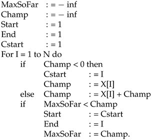
3. The Linear Algorithm Bentley Gave Me Credit for

This algorithm recursively calculates “BestEndingHere” at each stage. Formally, it looks like this:

As in Algorithm 1, Algorithm 3 honors (a) by restarting in MaxEndingHere, and (b) by restarting immediately.

Algorithm 3 Same as Algorithm 4 in Bentley [5]

The next question is whether Algorithm 3 can be modified to give the start and end positions of an optimal subsequence. The following algorithm does that.

Algorithm 4 Algorithm 3 modified to report the start and end of an optimal subsequence

The correctness of Algorithm 3 can be seen by induction. If MaxEndingHere at I-1 is correct, then so is MaxEndingHere at I.

An input vector that has only negative numbers leads, using Algorithm 3, to a MaxSoFar of zero, and the empty set. In this particular, it differs in behavior from Algorithm 1. A result of 0 could also occur if the input is non-positive and includes at least one 0. Hence, an Algorithm 3 result of 0 is ambiguous.

Is this algorithm merely a toy? No, it has been used in applications. Its origin came from efforts to find two-dimensional regions of high response in images [5]. The two-dimensional case is substantially more difficult than the one-dimensional case because the input is not simply ordered. Nonetheless, some of the algorithms proposed for the two-dimensional case use Algorithm 3 as a subroutine [6,7,8,9]. The time complexity of these algorithms for an $r\times c$ input is ${\left[min(r,c)\right]}^2+max(r,c)$. An application of these methods to optical and radio astronomy is given in [10]. Of course there are analogous problems for arrays of arbitrary dimensions, but one has to expect algorithms to be slower and demand more memory as the dimensions increase.

The algorithm is also used in computational biology, for example, in [11,12,13]. These applications make use of the linear speed on long DNA chains.

Additionally, electrical bio-engineers have found it useful. The R-peak is one of the parameters used in the analysis of electrocardiogram (ECG) data. In a study of a prototype of a wearable ECG system, Xiang et al. [14] use a modification of the algorithm to capture and compress R-peak data.

Computer scientists have used the algorithm to explore string matching, which has many uses [15].

While these applications show that the algorithm is useful in certain problems, such applications are only part of the story. What explains that Leetcode has had 6.9 million downloads of the maximum subarray problem [16]?

The first answer, I believe, is its widespread use as an interview question for coders seeking employment. Leetcode introduces themselves as “the best platform to help you advance your skills, expand your knowledge and prepare for technical interviews." Why would this be an attractive question to test a candidate coder? The problem is easy to state. The algorithm is simple to code, if the candidate understands it. Additionally, there are various ways of disguising it, such as proposing an array of positive numbers, and asking for the subarray with the largest product.

There is a second answer as well. The algorithm is an application of dynamic programming. For teaching purposes, it can be introduced as a simple example of dynamic programming, a powerful method when it applies [17].

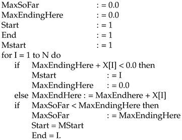
4. Comparing Algorithms 1 and 3

These algorithms look very similar. The driving mechanism of Algorithm 1 is

$$\mathrm{Champ}=\mathrm{X}\left[\mathrm{I}\right]+\mathrm{Max}(0.0,\mathrm{Champ}),$$

(1)

while that of Algorithm 3 is

$$\mathrm{MaxEndingHere}=\mathrm{Max}(0.0,\mathrm{MaxEndingHere}+\mathrm{X}[\mathrm{I}\left]\right).$$

(2)

To make them look even more similar, (1) can be rewritten as

$$\mathrm{Champ}=\mathrm{Max}\left(\mathrm{X}\right[\mathrm{I}],\mathrm{Champ}+\mathrm{X}[\mathrm{I}\left]\right).$$

(3)

Nonetheless, they are different. The relationship between the two algorithms is given in the following proposition:

$$\mathrm{MaxEndingHere}=\mathrm{Max}(0,\mathrm{Champ}).$$

(4)

The proof of (4) is given in Appendix A.

Corollary to Proposition: If the input array X has at least one positive element, then the maximum sum subarrays found by Algorithms 1 and 3 are equal. The proof of the corollary is also in Appendix A. The corollary shows that Algorithms 1 and 3 can differ only in the case of an all non-positive input.

Table 1. Comparison of Algorithms 1 and 3.

	Algorithm 1	Algorithm 3
Time	0 (n)	0 (n)
Space	0 (1)	0 (1)
Correct?	Yes	Yes
Modify to report start and end	Algorithm 2	Algorithm 4
Negative input	Either empty set or
	largest element	Empty set only

compares the two algorithms.

I slightly prefer Algorithms 1 and 2 to Algorithms 3 and 4 because they handle the all-negative-input case more smoothly.

5. Discussion

Memories are tricky things. Bentley (private communication) was writing their column some five years after the seminar. He believes that at the time of the seminar he understood my algorithm to be Algorithm 1, but that his later reconstruction of it resulted in Algorithm 3. That it took 40 years to recognize that such a misunderstanding had occurred is entirely on me.

We now have two similar but different light-weight algorithms for the maximum subarray problem. Even though algorithmically they are virtually identical, they reflect different ways of thinking about the maximum subarray problem. That there are two is a gain in our knowledge, and raises new questions. Are there other such algorithms that are similarly light-weight, or are these two unique in some sense? Can the ideas behind these algorithms aid in the two-dimensional problem of Grenander, either with an exact algorithm or heuristically? Algorithms are continuously fascinating.

References

1. von Neumann, J.; Morgenstern, O. Theory of Games and Economic Behavior; Princeton University Press: Princeton, NJ, USA, 1944. [Google Scholar]
2. Savage, L. Foundations of Statistics; J. Wiley and Sons: New York, NY, USA, 1954. [Google Scholar]
3. Dantzig, G. Linear Programming and Extensions; Princeton University Press: Princeton, NJ, USA, 1963. [Google Scholar]
4. Klee, V.; Minty, G.J. How good is the simplex algorithm? In Inequalities III, Proceedings of the Third Symposium on Inequalities, Los Angeles, CA, USA, 1–9 September 1969; Dedicated to the Memory of Theodore S. Motzkin; Oved, S., Ed.; Academic Press: New York, NY, USA; London, UK, 1972; pp. 159–175. [Google Scholar]
5. Bentley, J. Algorithm Design Techniques. Commun. ACM 1984, 27, 865–871. [Google Scholar] [CrossRef]
6. Maximum Sum Rectangle in a 2D Matrix. Available online: https://www.geeksforgeeks.org/maximum-sum-rectangle-in-a-2d-matrix-dp-27 (accessed on 2 November 2023).
7. Maximum Sum Rectangle in a 2D Matrix—Kadane’s Algorithm Application (Dynamic Programming). Available online: https://www.youtube.com/watch?V=FgseNO-6Gk (accessed on 2 November 2023).
8. Ray, T. Maximum Sum Rectangular Submatrix in Matrix Dynamic Programming/2D Kadane. Available online: https://www.youtube.com/watch?v=yCQN096CwWM (accessed on 2 November 2023).
9. Saleh, S.; Abdellah, M.; Abdel Raouf, A.; Kadah, Y. High Performance CUDA-based Implementation for the 2D Version of the Maximum Subarray Problem (MSP). In Proceedings of the 2012 Cairo International Biomedical Engineering Conference, Giza, Egypt, 20–21 December 2012. [Google Scholar]
10. Waddell, S.; Takaoka, T.; Read, T.; Candy, R. Maximum subarray algorithms for use in optical and radio astronomy. In Proceedings of the SPIE 8500 Image Reconstruction from Incomplete Data VII, San Diego, CA, USA, 12–16 August 2012. [Google Scholar] [CrossRef]
11. Rakocevic, G.; Semenyuk, V.; Lee, W.; Spencer, J.; Browning, J.; Johnson, I.J.; Arsenijevic, V.; Nadj, J.; Ghose, K.; Suciu, M.C.; et al. Fast and accurate genomic analyses using genome graphs. Nat. Genet. 2019, 51, 354–362. [Google Scholar] [CrossRef] [PubMed]
12. Zhao, J.; Song, X.; Wang, K. IncScore: Alignment-free identification of long noncoding RNA from assembled novel transcripts. Sci. Rep. 2016, 6, 34838. [Google Scholar] [CrossRef] [PubMed]
13. Wu, J.; Lee, W.P.; Ward, A.; Walker, J.A.; Konkel, M.K.; Batzer, M.A.; Gabor, T. Tangram: A comprehensive toolbox for mobile element insertion detection. BMC Genom. 2014, 15, 795. [Google Scholar] [CrossRef] [PubMed]
14. Xiang, J.; Dong, Y.; Xue, X.; Xiang, H. Transactions on Biomedical Circuits and Systems; IEEE: New York, NY, USA, 2019; Volume 13, pp. 68–79. [Google Scholar]
15. Aygun, R. Using Maximum Sum Subarrays for Approximate String Matching. Ann. Data Sci. 2017, 4, 503–531. [Google Scholar] [CrossRef]
16. Available online: https://leetcode.com/problems/maximum-subarray/ (accessed on 2 November 2023).
17. Miriello, B. Kadane’s Algorithm: Gateway to Dynamic Programming. 2020. Available online: https://levelup.gitconnected.com/kadanes-algorithm-gateway-to-dynamic-programming-26e95ec13c7f (accessed on 2 November 2023).