Article

Supervised Methods for Modeling Spatiotemporal Glacier Variations by Quantification of the Area and Terminus of Mountain Glaciers Using Remote Sensing

by
Edmund Robbins
1,†,
Thu Thu Hlaing
1,†,
Jonathan Webb
2 and
Nezamoddin N. Kachouie
1,*,†
1
Department of Mathematics and Systems Engineering, Florida Institute of Technology, Melbourne, FL 32901, USA
2
Department of Mathematics and Statistical Science, University of Idaho, Moscow, ID 83844, USA
*
Author to whom correspondence should be addressed.
These authors contributed equally to this work.
Algorithms 2023, 16(10), 486; https://doi.org/10.3390/a16100486
Submission received: 30 August 2023 / Revised: 9 October 2023 / Accepted: 12 October 2023 / Published: 19 October 2023
(This article belongs to the Special Issue Supervised and Unsupervised Classification Algorithms (2nd Edition))

Abstract

:
Glaciers are important indictors of climate change as changes in glaciers physical features such as their area is in response to measurable evidence of fluctuating climate factors such as temperature, precipitation, and CO2. Although a general retreat of mountain glacier systems has been identified in relation to centennial trends toward warmer temperatures, there is the potential to extract a great deal more information regarding regional variations in climate from the mapping of the time history of the terminus position or surface area of the glaciers. The remote nature of glaciers renders direct measurement impractical on anything other than a local scale. Considering the sheer number of mountain glaciers around the globe, ground measurements of terminus position are only available for a small percentage of glaciers and ground measurements of glacier area are rare. In this project, changes in the terminal point and area of Franz Josef and Gorner glaciers were quantified in response to climate factors using satellite imagery taken by Landsat at regular intervals. Two supervised learning methods including a parametric method (multiple regression) and a nonparametric method (generalized additive model) were implemented to identify climate factors that impact glacier changes. Local temperature, CO2, and precipitation were identified as significant factors for predicting changes in both Franz Josef and Gorner glaciers. Spatiotemporal quantification of glacier change is an essential task to model glacier variations in response to global and local climate factors. This work provided valuable insights on quantification of surface area of glaciers using satellite imagery with potential implementation of a generic approach.

1. Introduction

The mountain cryosphere and the glaciers found around the globe have a non-trivial impact on humanity. On a fundamental level, the glaciers scattered throughout the globe, provide a large segment of the world’s residents with a source of freshwater. Populations residing in arid regions, typically near mountains often depend on run off from melting glaciers for their water during the drier and warmer parts of the year. River systems meandering through portions of Asia are sustained from ice and snowmelt located in the Himalayas and the glaciers within the mountain range, this is particularly true in late summer when a predominant factor contributing to river flow comes from melting glaciers [1] provides a supplementary source of water during the sustained dry periods experienced in this urban region [2]. The socio-political impacts due to the loss of mountain glaciers have the potential to be significant on both the ecological and global political level [3]. The recognition of these contingencies has spurred increased interest and research into the study of the mountain cryosphere and the health of the glacier it contains.
Stepping into the issue of glacier recession one quickly realizes the enormity of the undertaking this problem set. The first roadblock is the substantial number of glaciers that can be found around the globe (Figure 1). The Global Land Ice Measurements from Space (GLIMS) Glacier Database currently has 604,986 unique glacier outline entries [4,5]. Investigation of the spatial data demonstrates that many individual glaciers are but one component of a complex subsection of a larger glacier network (Figure 1). Additionally, the remote, and in some cases, denied locations, coupled with austere conditions found in the vicinity of glaciers places emphasis on finding alternatives to the in-situ measurements of changes taken on the ground. An example would be the country of North Korea, obtaining access to glaciers here may prove challenging or impossible.
One candidate for a collection method which finds extensive use in the existing literature is remote sensing, and more specifically the use of satellite imagery. Remote sensing is a broad-based term that encompasses a diverse number of platforms which include both spaceborne platforms on orbit and air breathing aerial platforms which include assets like drones or aircraft equipped with different sensor technology. The existing datasets and databases contain multiple decades of useful images from which to extract information. Within these images the features of principal interest are the location of the glacier’s terminal point (Figure 2) and its change through time. The proper identification of which allows for the estimation of the recession velocity along with the changing area of the glacier or glaciers of interest. Found within the extant literature, are numerous methods for estimating changes in the location of a glacier’s terminus using optical based image data and for estimating changes in glacial area [6,7,8,9].
Previous research on methods of glacial recession and on the identification of glacial termini are vast. The work has produced numerous methodological processes using a variety of diverse techniques (Figure 2). Surveying these efforts, one can glean that while some of the methods will work well on single efforts or one-off projects, for instance a study of one particular glacier, others are more suitable for larger scale analysis and have the potential to be easily automated and generalizable. Given the size of the global glacier inventory is a desirable quality for global scale of modeling. Previous research using commonly employed methods to track changes in the termini of glaciers has shown a common theme. This commonality is the reduction of what is in the final analysis, a three- dimensional (3-D) spatial phenomena being projected down to a zero-dimensional (0-D) spatial value for the terminus location to evaluate the distance the glacier has advanced/retreated along its path of motion. This dimensionality reduction provides a level of efficiency in the analysis of the glacier motion and is a useful model simplification when it is appropriate. A comparison of standard methods including the center-line, bow, rectilinear-box, curvilinear-box, and extrapolated is provided by Lea et al. 2014. Each of the above-mentioned methodologies is subject to its own advantages and weaknesses and the use of any one of the methods involves considerations of glacial geometry along with the aim of the study being undertaken [10].
Other work applies a more general approach to terminus estimation which relies heavily on optical imagery. An advantage of which is to avoid specific geometric dependencies of a particular glacier. The method exploits the properties of the multiband attributes of satellite imagery and the flexibility of Nonparametric Regression [7]. Taking advantage of the return times of the LANDSAT satellite platform, this method uses selected spectral bands of the images to identify which regions of the spectrum produce the largest intensity changes along the path of the glacier. This intensity change is indicative of the transition from soil, vegetation, and debris of the mountain landscape to the ice of the glacier. These intensity changes are collected through time as this process is repeated on a series of images. On each image a glacier path is manually drawn, this path is simply a hand drawn curve. Then along the length of this path the intensity of each pixel is collected. Using the derivatives and the inflection points of the collected intensity values to identify the terminal points of the glacier, the method can capture the glacier movement against a ground truth, based on direct measurements.
A major drawback to this method is its dependency on an investigator drawing the path of the glacier manually. As was mentioned previously this would make the method problematic in large scale glacier networks, or global glacier studies. It would also prevent, in its current state, an automated implementation given the dependency on a human drawn path to derive the intensity profile. It is with the final goal of limiting or eliminating manual input that this papers current methodology was developed. In addition to increasing ease of automation, robust and flexible models for estimating glacier variations in response to global and local climate factors is developed by either detection of the glacier terminal point or quantification of the glacier area.
The objectives of this research are to implement a generic method for quantifying glacier area and locating its terminus and model their variations in response to climate factors using both parametric and nonparametric supervised techniques. The geometry of individual glaciers has been estimated using remote sensing techniques to include various semi-automated image analysis techniques such as supervised classification, edge detection, and region segmentation in an attempt to develop a pipeline for quantification of glacier changes that could be potentially applicable to a large set of glaciers around the globe.

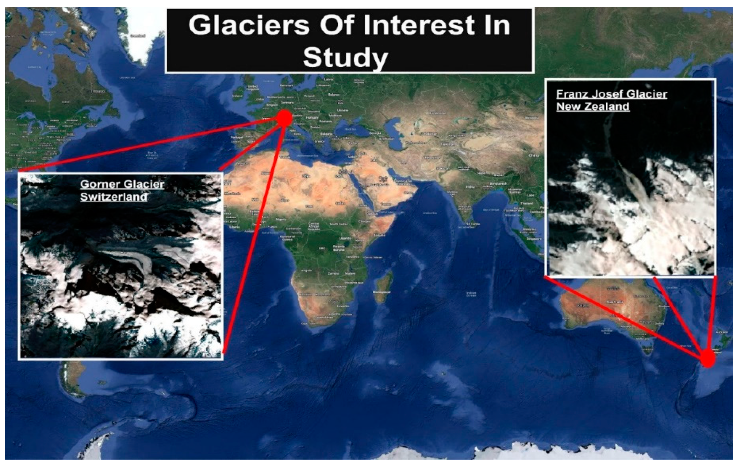
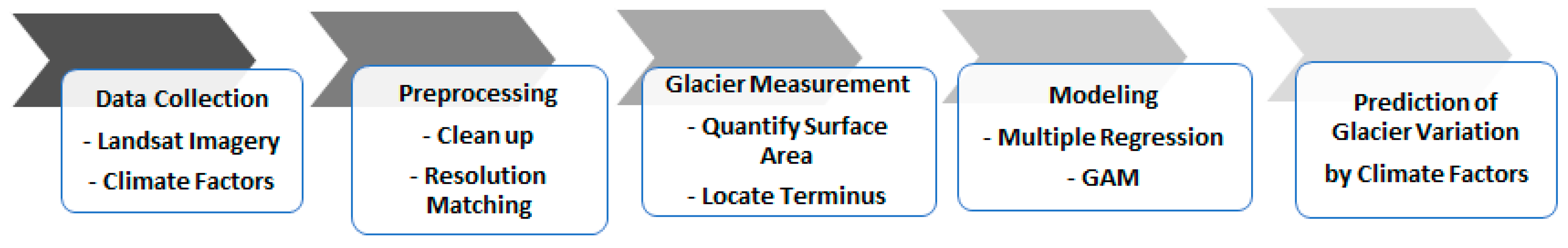
2. Data Collection and Preprocessing

Two distinct types of data were employed to study the glacier recession by quantifying changes in the terminal point and area of Gorner and Franz Josef glaciers (Figure 3). These are two similar but spatially distant mountain glaciers. One set of data consists of satellite imagery, multiple images of spatial locations taken over time. The other data type is a univariate time series of environmental sensor recordings of multiple climate factors collected by various international agencies. Each of the data sets presents its own challenges from a data wrangling perspective given the diversity of values, measurement scales, and potential usefulness of the attributes unique to each data type.

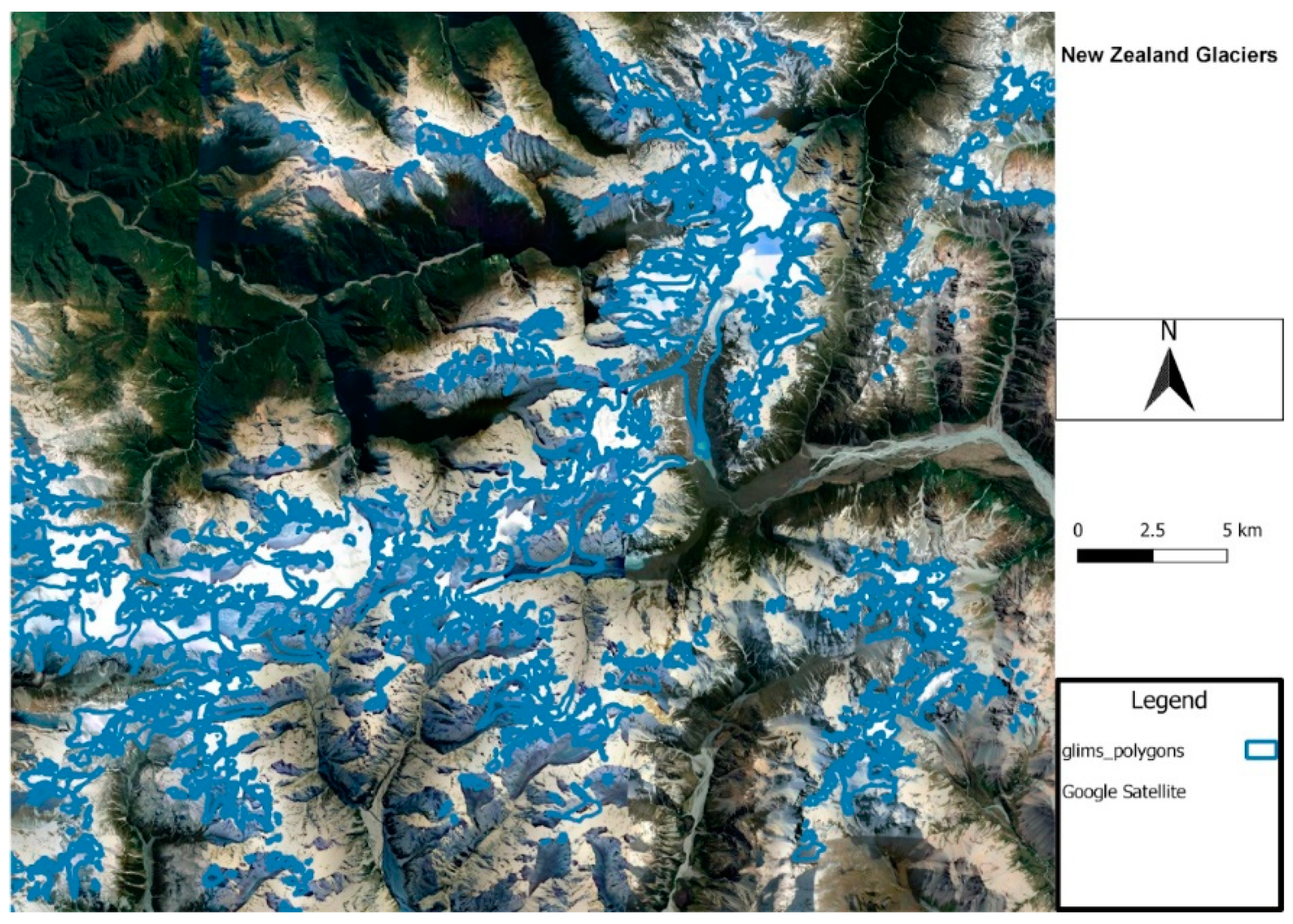
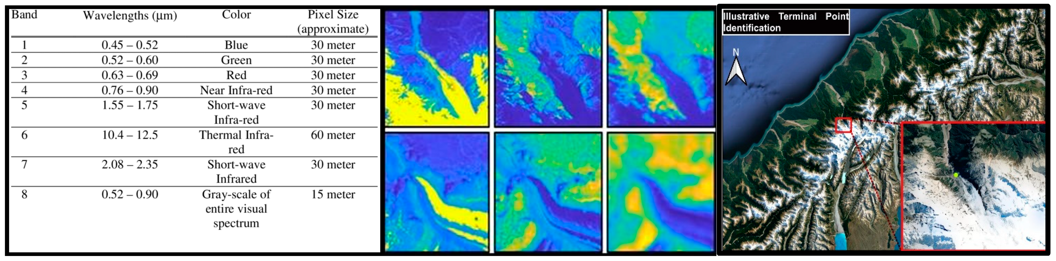
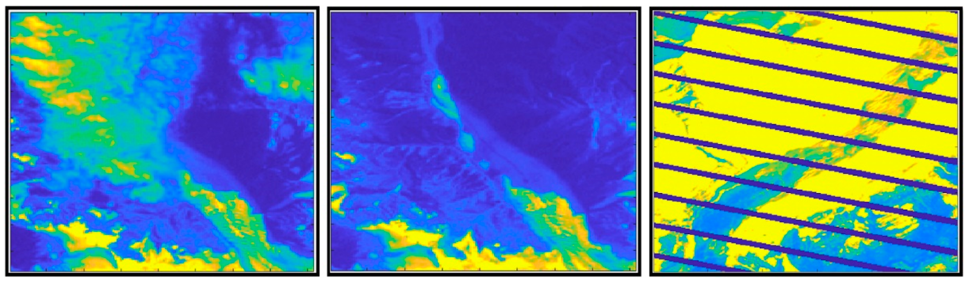
2.1. Landsat Imagery

The main source of imagery used in this study is satellite imagery of the glaciers of interest gathered exclusively via the Landsat program publicly available through the National Aeronautics and Space Administration’s (NASA) [11]. The Landsat data is stored in online databases and is freely accessible and downloadable via the web. The Landsat images along with the metadata (and much more) are available via the United States Geological Survey’s Earth Explorer webpage found at https://earthexplorer.usgs.gov/ (accessed on 16 February 2021). It must be pointed out that, Sentinel program sponsored by European Space Agency provides satellite imagery with better resolution (in some spectral bands) taken by Sentinel-2 satellite. However, the Sentinel program began in 2015 and an inventory of only about 8 years of satellite imagery is available through this program. In contrast, the Landsat program started in 1972, provides more than 5 decades of data available. Moreover, satellite imagery with better resolutions is only available commercially for a much shorter period than a decade.
The images of each glacier are captured at specific dates based on the glacier’s geographic coordinates. Landsat has a 16-day return time, and the data is collected over several decades. The data has been publicly available since 2008 which has made it an attractive database of satellite imagery for scientists performing multidecade studies. In the preprocessing step of this study, we removed those scenes where the glaciers were obscured by clouds or mountain shades, and scenes with degraded imaging due to sensor malfunctioning. An example of image degradation can be found in the Landsat 7 (one of the multiple Landsat platforms with available data) image products. After launch, the Scan Line Corrector (SLC) went off line and due to this malfunction images will contain a zig-zag pattern. This becomes an issue when the pattern intersects with the object of interest as it is depicted in Figure 4.
The Landsat images are collected with a multispectral sensor. This capability implies that each of the images contains several spectral bands. Each of these spectral bands has its own wavelength range of the electromagnetic spectrum. Multispectral imaging capability enables different views of the same scene highlighting features of interest that could be better viewed in created image in a specific band.
Figure 5 shows the specific breakdown of a typical multispectral Landsat 7 image into its spectral bands as well as band specific images in false color along with terminus localization process. In this analysis the dataset was created from a collection of Landsat 7 and 8 images for both glaciers under consideration. The initial data pull consisted of 511 images in total for both glaciers, 263 for Franz Josef and 248 for Gorner. All of the original images fall in the date range January 2000 through November 2021. After cleaning the data for images where the glacier was obscured by clouds or shadows the final data sets for each glacier were as follows: Franz Josef data range is August 2000 through August 2021 and in this time frame 93 useful images were retained, while for Gorner the date range is May 2000 through October 2021 with 97 useful images retained.

2.2. Climate Factor Data

The climate factor data, which is used extensively in the modeling and prediction of the glacier variations, is time series data collected by several different sensors. The specific factors selected for the analysis were temperature in degrees Celsius, Carbon Dioxide (CO2) concentration in parts per million (ppm) and Precipitation in millimeters (mm). Each of these factors were collected by the appropriate national agencies with daily sampling frequency in the regions containing the glaciers in this study.
Daily climate data was collected from the weather station closest to Franz Josef and Gorner glaciers from the National Oceanic and Atmospheric Administration Climate Data Online platform available at https://www.ncdc.noaa.gov/cdo-web/datasets/GHCND/stations/GHCND:NZ000936150/detail (accessed on 7 July 2022). The data for Franz Josef was taken from the Hokitika Aerodrome weather station in New Zealand and spans the two decades from 1989 to 2009. For the Gorner glacier, the dataset was from the Sion weather station in Switzerland spanning from 1985 to 2009. The dataset contains daily information on minimum, maximum, and average temperate, and precipitation. To attain comparable resolution for the response, i.e., glacier variations estimated using spatiotemporal satellite imagery, and the predictors, i.e., climate factors, monthly data was calculated by averaging observed daily climate factors in the data preprocessing phase.
To assess the predictive viability of CO2 on glacier variations in the modeling process, the monthly Mauna Loa CO2 average data was sourced from NOAA. The sourced data contains monthly average CO2 levels from March 1958 to May 2021 recorded at the Mauna Loa station in Hawaii. The data is a proxy for many other human activities that contribute to climate change and the warming temperatures on the globe. Local temperature for each glacier was sourced from the closest regional station. An overall monthly global average temperature was also calculated in order to assess the overall temperature variations. A monthly data set was utilized from NOAA which contains samples of the monthly average temperature from January 1880 to December 2021. The result is a data set which contains a total of six predictors measured at both the global and local levels. Next, glacier variations (estimated either by detected terminus or by quantified area) will be modeled in response to monthly measurements of the predictors of interest (aforementioned data) for identification of potential relationship between temporal glacier variations and climate factors.

3. Methods

Due to the limitations of the previous methods for identification of glacier terminal points, along with the estimation of area, different techniques are required to improve the analytical process [10]. This work is a combination of image processing techniques with parametric and nonparametric statistical methods to model glacier change. In this section, a novel method, both in its breadth of analysis (area and terminal point) and generalizability (not designed for a specific glacier), will be discussed. First the investigative processes for quantifying changes in the terminal point and area variation of mountain glaciers will be developed, followed by the results of a preliminary application on two similar but spatially distant mountain glaciers (Figure 3). While both glaciers namely Franz Josef in New Zealand and Gorner in Switzerland share the characteristic of being mountain glaciers, they differ by being thousands of miles apart and in opposite hemispheres of the globe. This selection was deliberate in order to prevent the development of a model or a method that would rely on the characteristics of one specific glacier or geographical and climatological conditions found in one specific region.
The glacier termini are manually marked in the satellite imagery using a graphical user interface (GUI) developed in MATLAB R 2021b. After the identification of the terminal point the glacier area will be estimated via the application of several standard image processing techniques. This process is replicated over a time series of Landsat images. The results of both the terminal point locations and the estimated areas are stored for use as dependent variables in a model using climate factors as predictors to describe the variation in the glaciers attributes of interest (area and terminal point change). The overall intent of the modeling process is to construct a predictive and interpretable model for the variations of mountain glaciers due to global climate change and its effects. The schematics of the analytical process are displayed In Figure 6. The first step is data collection and preprocessing where Landsat imagery and climate data are collected, cleaned up, and preprocessed. This step also includes quantification of glacier area and localization of glacier terminus. Next, two different statistical approaches are taken, a parametric technique (multiple regression), and a nonparametric method (GAM). Both statistical approaches are applied to model glacier change. The glacier variation is once modeled using changes in spatiotemporal location of glacier terminus, and again by quantification of changes in glacier area over time.

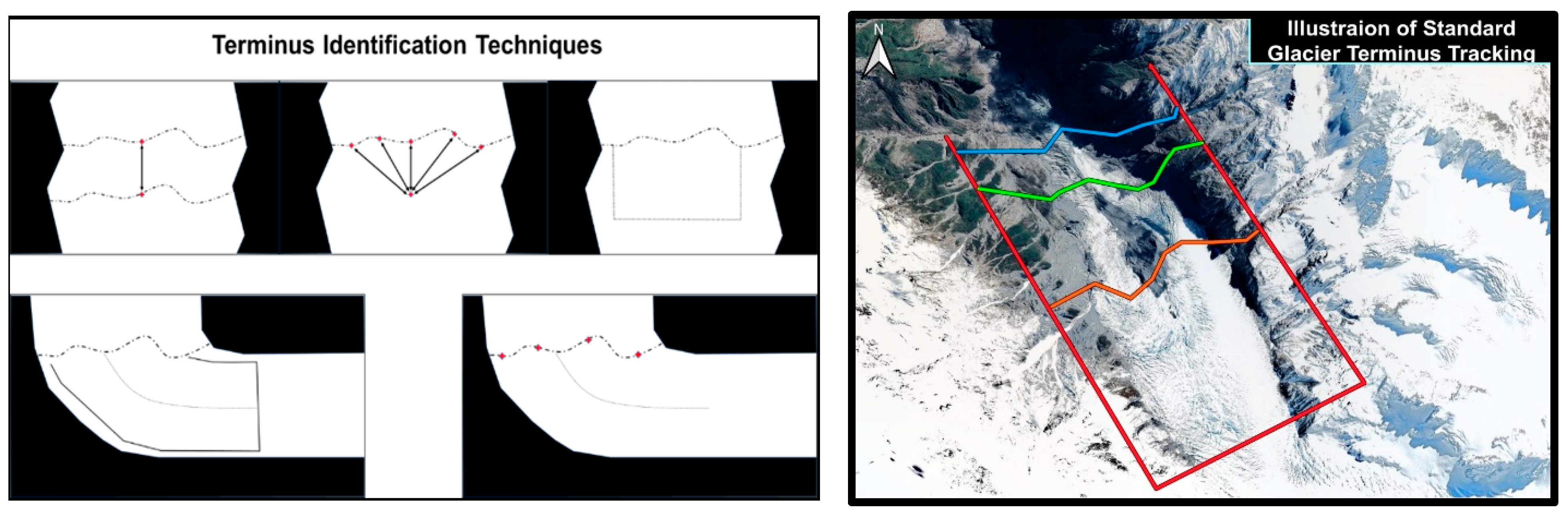
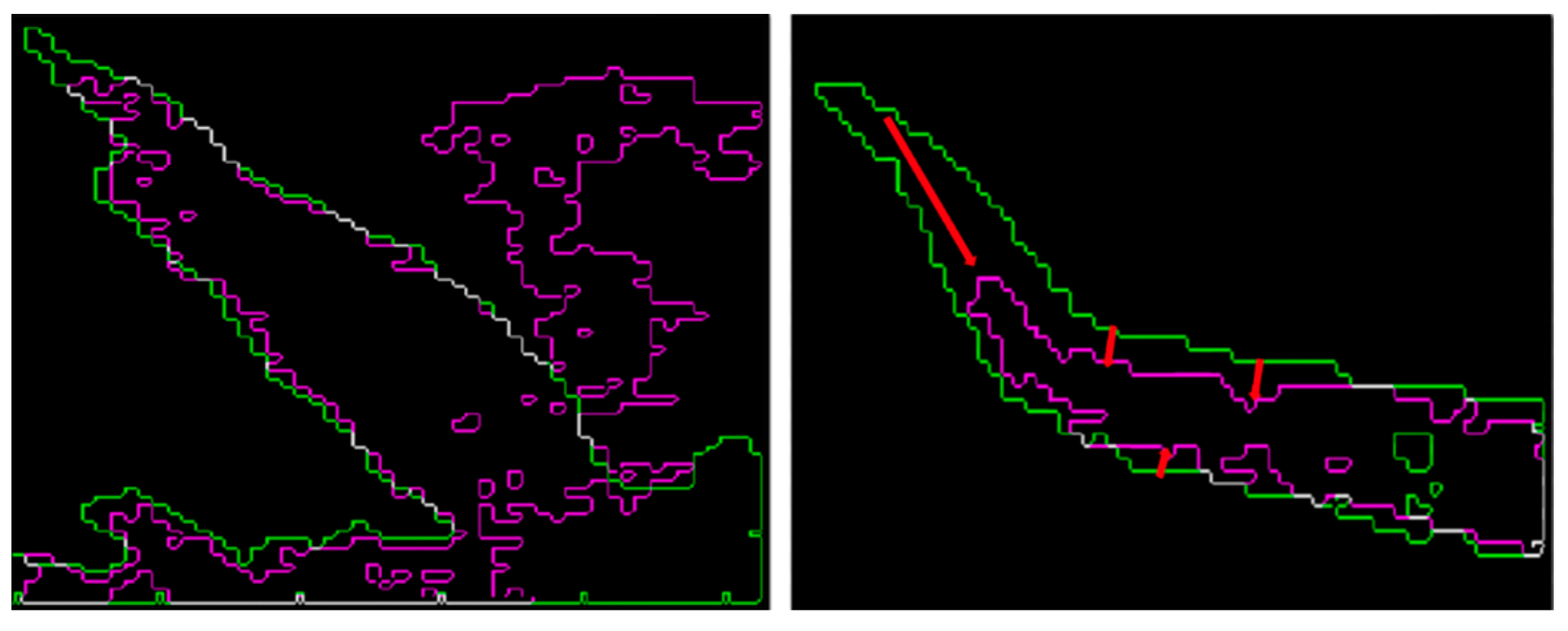
3.1. Quantification of Glacier Area and Terminus

Terminal point was located using a suit of image processing techniques over temporal sequence of images collected for each glacier. A graphical user interface was developed to zoom on the glacier’s geographical location on the image using glacier’s latitude and longitude. A bonding box as region of interest (ROI) encompassing the glacier’s area was drawn. The ROI was used to crop the glacier through entire sequence of original Landsat images. Terminal point location was then marked in each cropped image of the sequence.
Because only two glaciers were studied in this project, the manual terminus detection was an effective and rapid approach to locate the terminus and mark it by a single pixel on the glacier image. This manual detection method allowed a swift process of a large sequence of images for each glacier by avoiding issues such as partial obstruction of the glacier in the image.
Although an expedient method was developed for the identification of the terminus location, segmentation of glacier area proved to be a more challenging problem. This difficulty stem from the fact that finding the entire outline of the glacier is a two-dimensional problem in contrast with the detection of the terminal point that is a zero-dimensional task. The segmentation of cropped image to glacier and non-glacier segments with sharp boundaries is rather challenging due mainly to debris and mud blending into the ice near glacier’s boundaries.
Region growing and edge detection methods were preliminary attempted to segment the area of the glacier. Each of these methods were slightly successful to segment the glacier area. Region growing method creates homogenous regions based upon a specific threshold, while edge detection looks for abrupt changes in pixel intensity to identify an edge. A mutual challenge among both segmentation methods is to find the threshold for optimal segmentation of glacier boundary in each image in the sequence, one by one. Hence, a hybrid method was implemented by combination of region growing and edge detection techniques. Figure 7 shows some partially successful application of this hybrid Region Growing-Edge Detection approach to both glaciers in this study. Some regions containing both glacier and non-glacier areas can be observed in Figure 7(Left).
To further improve the segmentation results, a multi-level thresholding technique (Otsu’s method) was applied. Otsu’s method finds the optimum global threshold for the image segmentation by maximizing the between-class variance of the pixel intensities in the partitioned regions, here glacier vs. non-glacier. It demonstrated limited success in producing somewhat detailed depictions of the glacier in some images, but often could not produce sufficient separation between glacier and neighboring non-glacier areas.
The final approach contained three steps and outperformed the previous methods that were used for glacier segmentation in this study. In the first step, the images were cropped to remove as much of the glacier’s surroundings as possible. This cropping process has the virtue of reducing the surrounding non-glacier features to improve the segmentation results. The second step was to binarize the cropped image for preliminary segmentation of image to glacier and non-glacier partitions. The final step was the application of Otsu’s method for a detailed segmentation by finding the optimal global threshold. Different glacial regions in the binarized image were compared (by counting the number of pixels in each) to choose the region comprising the largest connected glacier area. The selective cropping in the first step greatly facilitated the performance. The main advantage of this technique was the combination of initial and final elimination of non-glacier areas.

3.2. Statistical Modeling

Beyond trying to identify glacier terminal points and glacial areas, the central point of the analysis is to identify the association between glacier terminus variation (as well as glacier area variation) and larger global dynamics specifically global warming driven by climate change. To this end, several potential models were developed to assess and analyze the potential association between the response and predictors.

3.2.1. Multiple Regression

First, multiple regression was implemented for modeling glacier variation using climate factors. For each glacier two separate models were constructed, one for each of the measured response variables, i.e., terminal point and glacier area. The general form of multiple regression model is:
y = B 0 + B 1 x 1 + B 2 x 2 + + B K x K + ε
where B i s are the unknown coefficients, x i s are the observed values of the predictors, and ε is the Gaussian error term. The multiple regression to model terminus location is:
d = B 0 + B 1 · C O 2 + B 2 · T M I N + B 3 · T M A X + B 4 · P R C P + B 5 · G l o b a l _ T e m p + ε
where d is temporal change of terminus (distance), TMIN is minimum local temperature, TMAX is maximum local temperature, G l o b a l _ T e m p is average global temperature, and PRCP is average precipitation. In a similar way, the multiple regression to model glacier area is:
a = B 0 + B 1 · C O 2 + B 2 · T M I N + B 3 · T M A X + B 4 · P R C P + B 5 · G l o b a l _ T e m p + ε
where a is glacier area.

3.2.2. Generalized Additive Model (GAM)

Because of the observed non-linear trends in glacier variations, the more advanced method of generalized additive models (GAMs) was implemented. GAM is a powerful nonparametric method that can potentially discover the complex nonlinear trends in the glacier variations. GAMs are more flexible than linear models and more interpretable than deep learning methods. GAM is essentially an additive model of nonparametric smooth functions [12,13,14]
g ( E Y X ) = f 0 + j = 1 K f j x j
where f ( x ) is a smooth function of predictor X , and Y is the response variable with a distribution belongs to the exponential family (ex. Gaussian, Binomial, Gamma, etc.). The main advantage of GAM is its capability to model highly complex and nonlinear relationships. The consideration and the associated tradeoff between the simplicity of a model and its interpretability. GAMs relax the restriction that the relationship must be a simple weighted sum, like in the multiple regression model, and instead assume that the outcome can be modeled by a sum of arbitrary smooth functions of each predictor variable.
The function g (   ) in the GAM model (Equation (4)) is known as the link function. The GAM links the sum of the smoothed predictors with the mean value of the assumed distribution using the link function g (   ) , which can be chosen flexibly depending on the problem under consideration. In addition to the Exponential family of distributions and the link functions, the third essential component to the GAM is the smoothing functions f j x j for the predictor variables in the model. This implies that the predictor variables become smooth curves by some function f. This is achieved for each of the functions f j x j in the GAM by using a basis of splines to create the nonparametric smooths using the Restricted Maximum likelihood method [14,15,16]. The GAM method employed in the current research regresses the terminus change by:
d = f C O 2 + f T M I N + f T M A X + f P R C P + f ( G l o b a l _ T e m p ) + ε
and the area change in the glaciers against the climate factors:
a = f C O 2 + f T M I N + f T M A X + f P R C P + f ( G l o b a l _ T e m p ) + ε
In both GAM models in Equations (5) and (6), the distribution selected from the exponential family is the Gaussian. This distributional assumption leads to the link function being the identity function. The basis functions for the nonparametric smoothing are Thin-Plate Splines where the dimension of the basis is varied from two to four basis functions over selected permutations of predictors in the model. The smoothing selection method REML is applied for smoothness selection. This leads to the functional form of the applied GAM for the glacier recession analysis. Subsets and permutations of the smoothed predictors will be evaluated against the full model using the Akaike Information Criterion (AIC) for model selection. The top performing GAM for each independent variable, terminal point distance, and area will be the model with lowest AIC value.

4. Results

After quantification of glacier area and locating its terminus, a univariate time series for the changes in Franz Josef and Gorner glacier’s terminal point and area were created from the collected Landsat image sequences. The climate data provides the independent variables for both the multiple regression and the GAM while the area, and location data are used as the response variable. Multiple regression and GAM were used for modeling the glacier variations. As depicted in Figure 8, it can be observed that the two glaciers have differing behaviors over the time. Franz Josef having a period where the glacier was advancing while Gorner was in a continuous state of retreat during the same period (1985–2010). The optimal multiple regression based on AIC for modeling Franz Josef variations was a combination of local temperature, global temperature, CO2, and average precipitation for terminal point as response, and only local temperature and average precipitation for area as response (Table 1). Local temperature and CO2 were identified as the impactful factors by multiple regression to model Gorner glacier variations using terminal point, while with glacier area as response, local temperature and global temperature were only impactful predictors identified by the model (Table 1). The optimal GAM for modeling Franz Josef variations was a combination of local temperature, CO2, and average precipitation using either terminal point or glacier area as response (Table 2). Local temperature, average precipitation, and CO2 were identified as the impactful factors by GAM to model Gorner glacier variations using terminal point, while with glacier area as response the global temperature was also included in the model (Table 2).
Figure 8(Top) displays a time series for the changes to the terminal point for Franz Josef (left) and Gorner (right) glaciers from the years 2000 to 2021. According to the left-hand side of Figure 8(Top), the time series for Franz Josef’s shows that the terminal point has oscillated between advancing and receding in the beginning years of 2000–2010. However, after the year 2000, it has been continuously receding; by 2021, the terminal point had receded close to 800 m by 2021 in comparison to its starting point in 2000. For Gorner glacier on the right-hand side of Figure 8(Top), the time series displays a continuous pattern of decline over the years from 2000 to 2021. By 2021, the terminal point has receded close to 500 m in comparison to its starting point in 2000.
When trying to measure the physical variations to both glaciers through their terminal point location, the data reflects that both glaciers have been receding significantly. As for the changes in area, for Franz Josef, the time series in Figure 8(Bottom) displays a similar oscillating behavior show in the corresponding one for terminal point, but overall, the area has decreased in 2009 when compared to 1989. The time series for Gorner glacier on the right-hand side of Figure 8(Bottom) continues to display a more straightforward receding effect as the area has been continuously decreasing from 1985 to 2009.

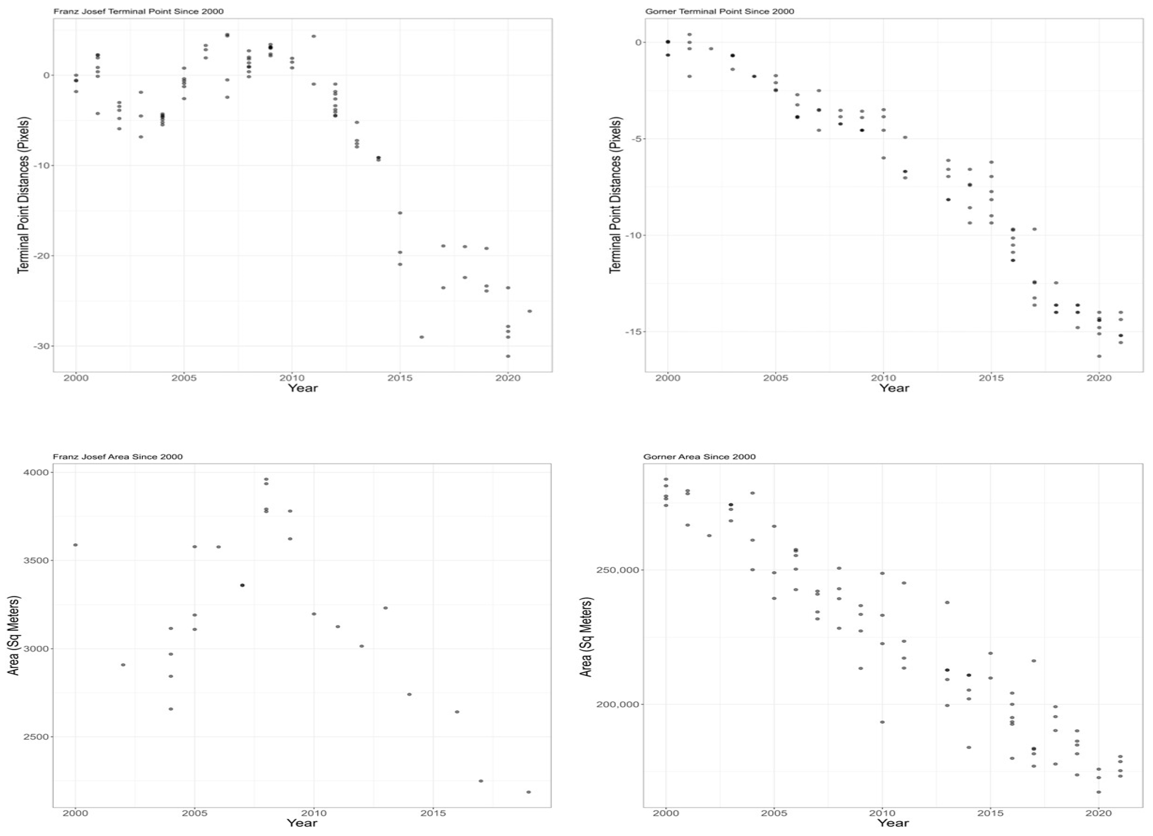
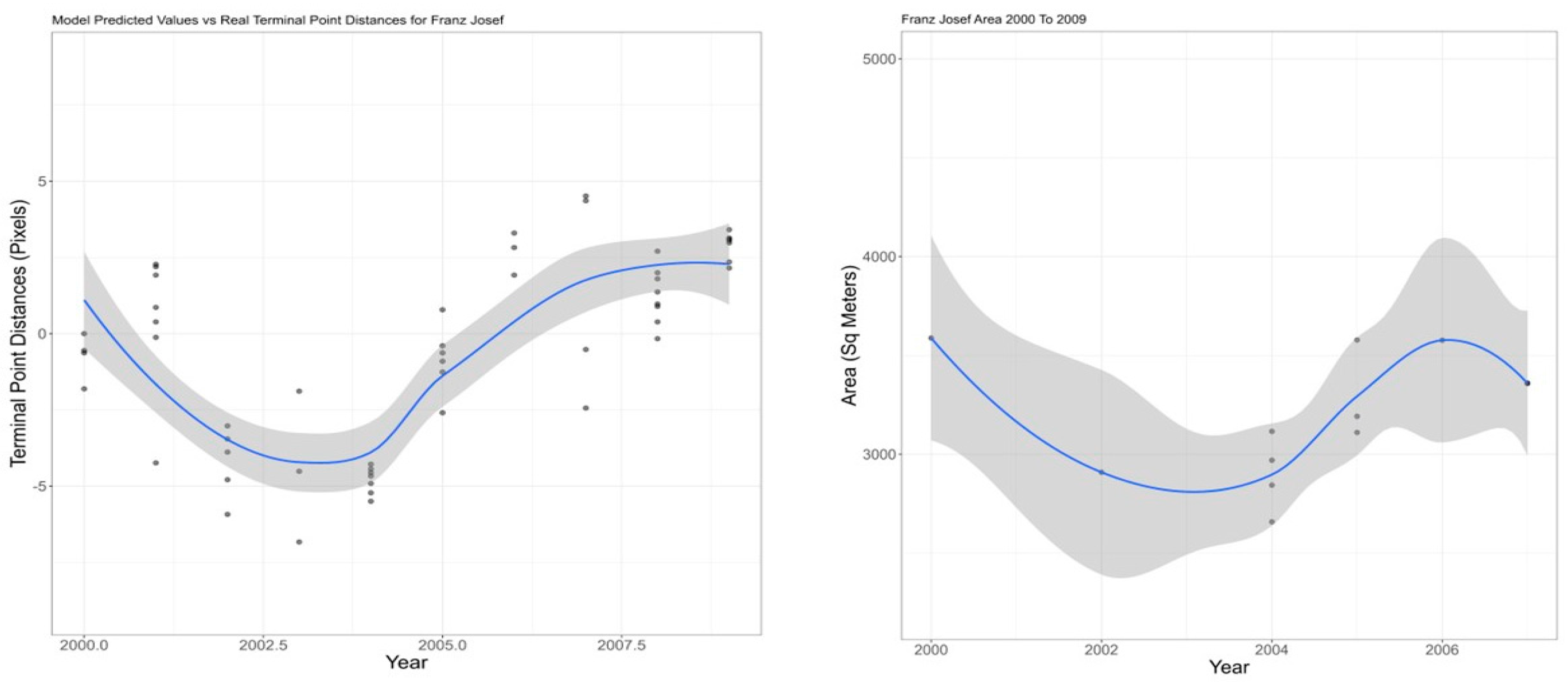
4.1. Modeling Variations in Franz Josef Terminal Point and Area Using Multiple Regression Model

Multiple regressions and generalized additive models introduced within the methods sections were explored to find which model could best explain the variations of both glacier’s terminal point and area presented above using climate factors. The best performing multiple regression to model Franz Josef’s terminus variations was a linear combination of precipitation, monthly average maximum temperature, global temperature, and CO2 with highest adjusted R 2 of 0.64, the lowest Akaike information criterion (AIC) of 555, and the lowest Singular Bayesian Information Criteria (SBIC) of 308 (Table 1a). The best multiple regression to model the variations in the area of Franz Josef could only achieve R 2 of 0.40 (Table 1b).

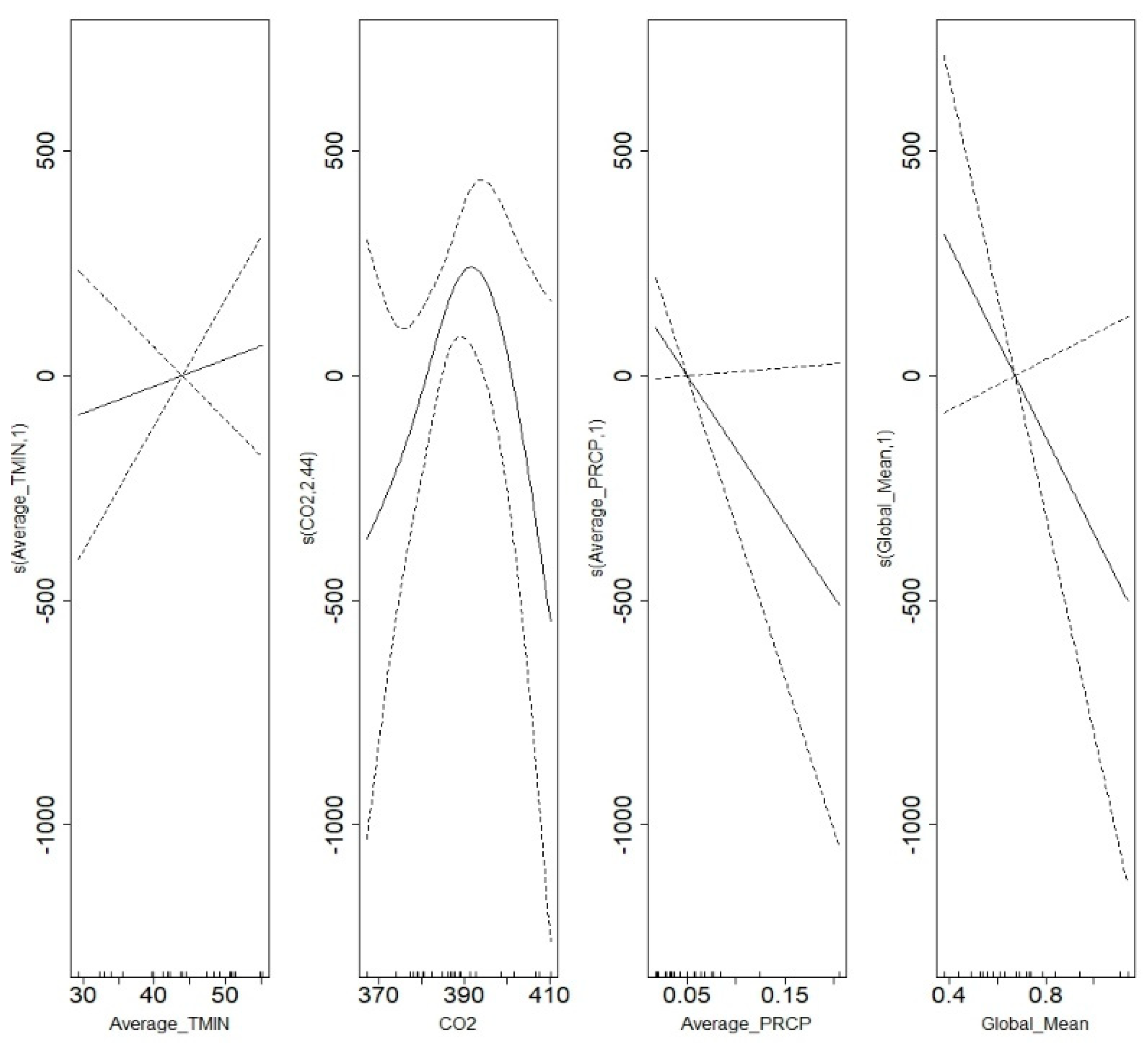
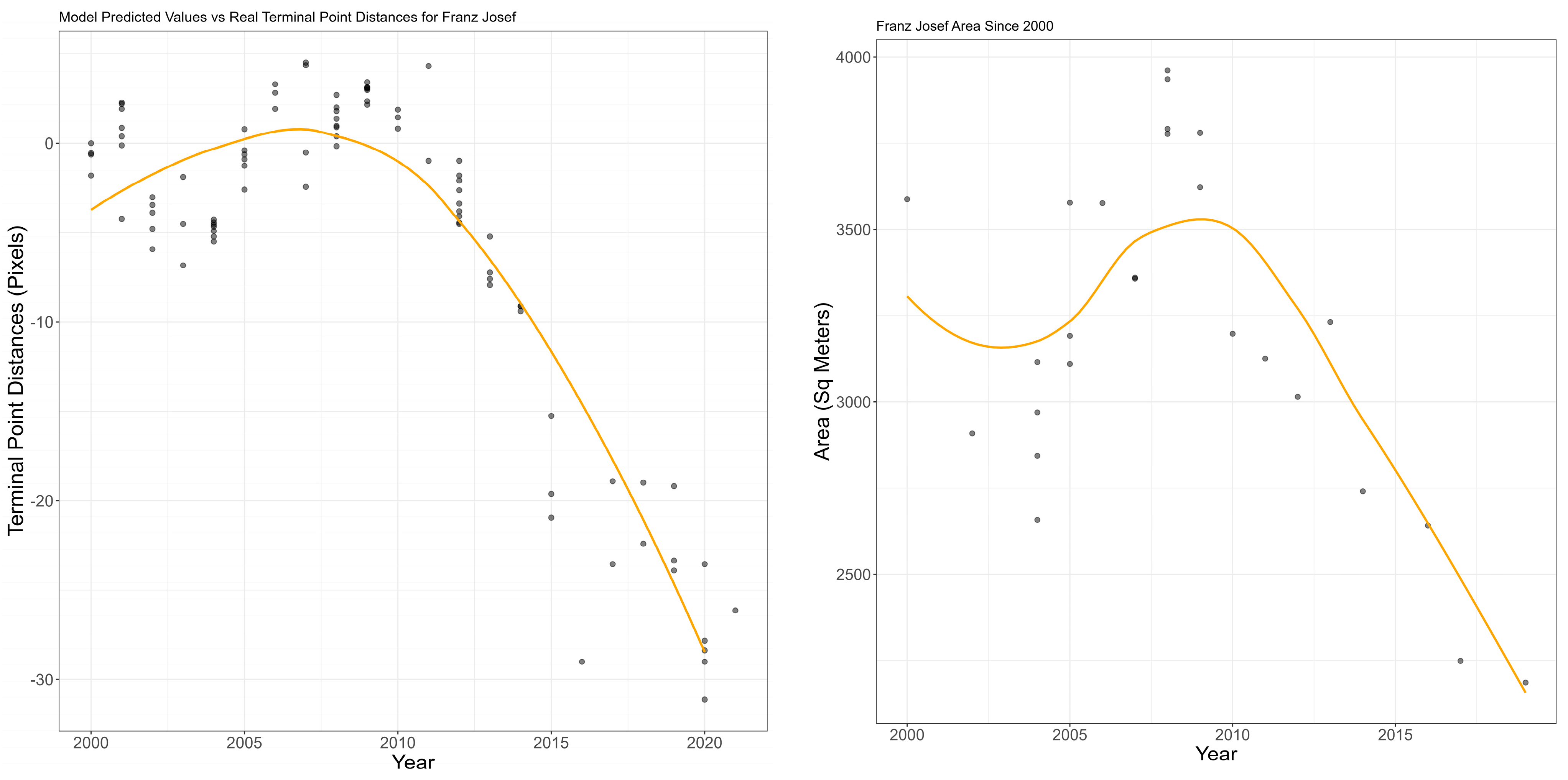
4.2. Modeling Franz Josef Terminal Point’s Variations Using Generalized Additive Model

Next, generalized additive models were implemented to address the shortcomings of multiple regression to model nonlinear trends. General additive models using different combinations of predictors were implemented and compared to find the significant predictors that could explain the variations in Franz Josef’s terminus. The best overall model was the linear combination of the smooth functions of average global mean, monthly average local minimum temperature, precipitation, and CO2 depicted in Figure 9(Left). The GAM had the highest adjusted R 2 of 0.85 and the lowest AIC of 481 (Table 2a), while the multiple regression only had the highest adjusted R 2 of 0.64 (Table 1a). As mentioned in the Methods section general additive models are the linear combination of nonparametric smooth functions. A visual representation of the smoothed function of the climate variables used within the model can be seen in Appendix B. The dashed lines within the figure represent the confidence intervals for each smoothed function. Model’s predicted output for the variation of Franz Josef’s area based on measured data is depicted in Figure 9(Left) and Figure 10(Left). When looking at how the model performed in terms of explaining the variations, it seemed to perform adequately, as the model shows a trend of recession followed by an advancement. Therefore, the observation of Franz Josef’s terminal point demonstrates that in overall Franz Josef has advanced between 2000 and 2009.

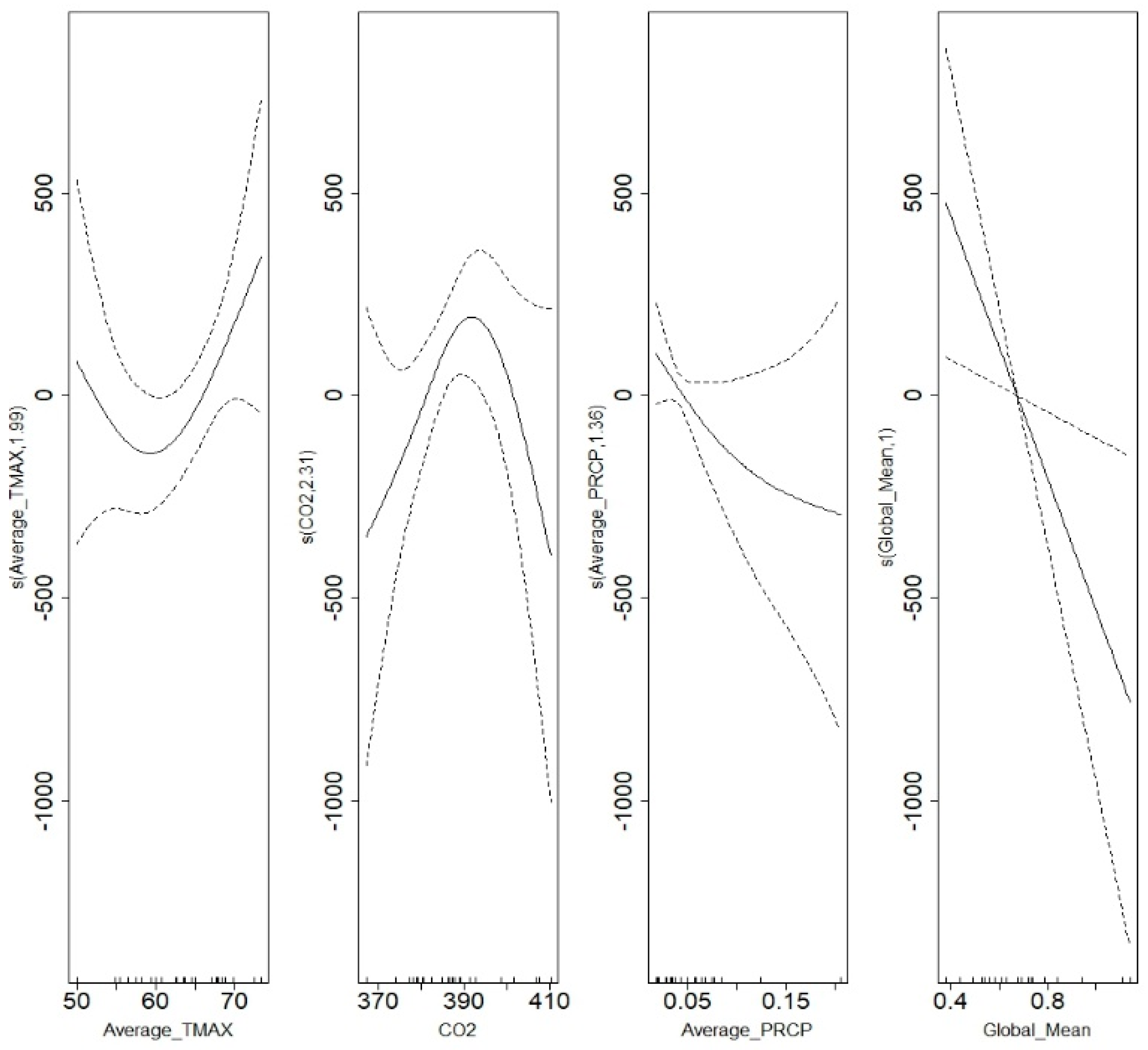
4.3. Modeling Variations in Area of Franz Josef Using Generalized Additive Model

To understand more about the behavior of Franz Josef glacier during this decade, variations of its area were also investigated. The best multiple regression model was able to only explain below half of variations with adjusted R 2 of 0.4. However, the best GAM was able to explain about 62% of the variability using average global mean, monthly average local maximum temperature, precipitation, and CO2 depicted in Figure 9(Right) and Figure 10(Right). A visual representation of the 4 smoothed functions contained with the GAM are displayed in Appendix B.
While the general shape of the local temperature and CO2 predictors have change, the precipitation and global temperature functions still remain liner. When comparing the model’s predicted outputs to the measured data (Figure 10(Right)), the model is shown to accurately capture the general trend of the data. In addition, when comparing this graph to the graph of Franz Josef’s model outputs for terminal point measurements (Figure 10(Left)), they look very similar. Both graphs seem to decrease from 2000–2004, and then increase right afterwards, which indicate that Franz Josef was actually advancing from 2004–2009 as shown by the increase in area and terminal point position.
This is abnormal behavior as the majority of glaciers around the globe were retreating during this time period. However, for exceptional cases such as the glaciers in New Zealand, there were periods of advancement in terms of both the area and terminal point as a result of the increased precipitation. As we can see in the Figure 10, the trend marked in orange is the smoothed function of the model’s predicted values, while the points are the measured data. From 2000 to 2009. The advancement that was observed in the Figure 9 can be seen in Figure 10 as well, however after the advancement, there is continuous recession. The model was able to generally explain the variations within the terminal point and area for Franz Josef glacier for the past two decades.

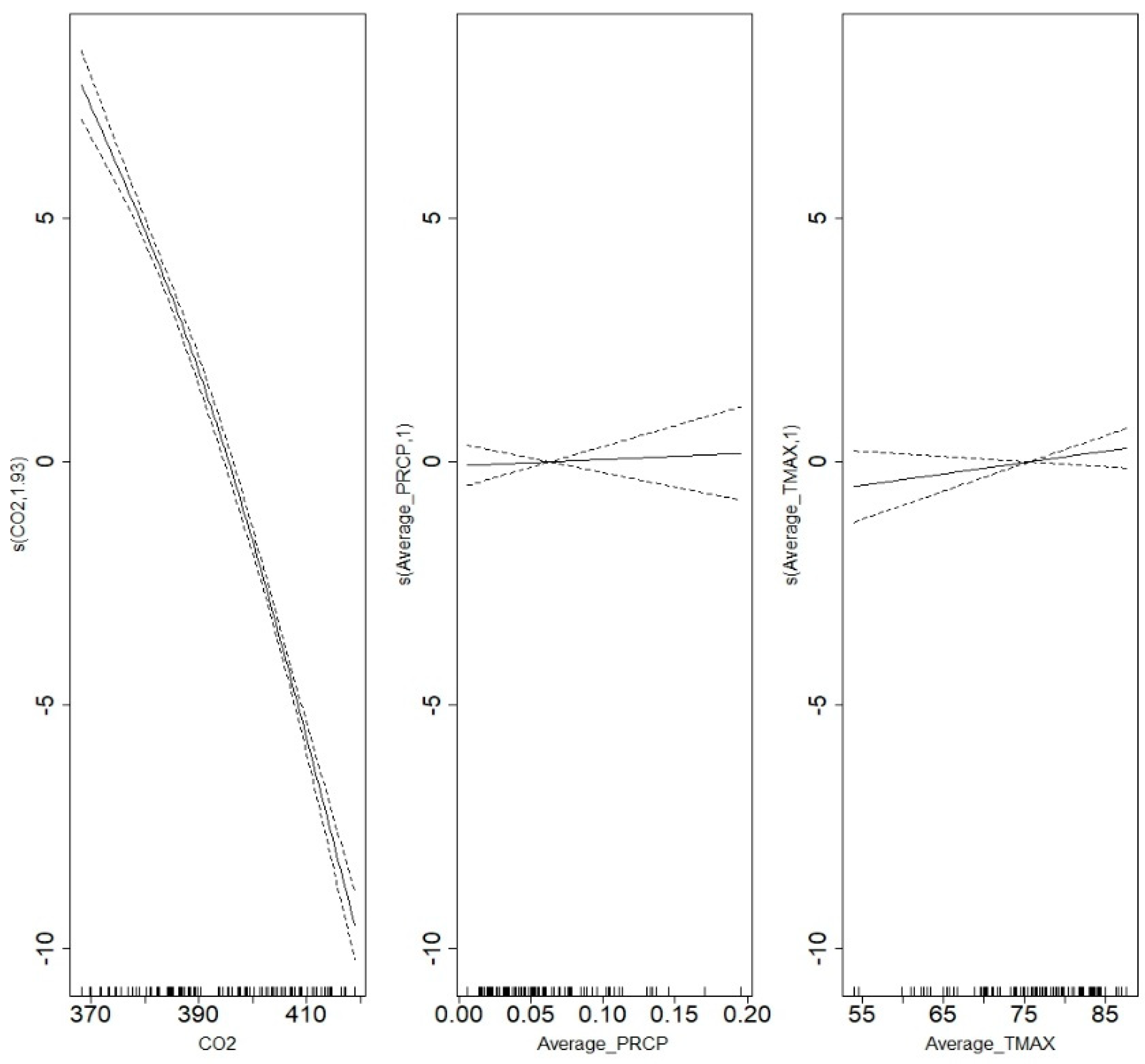
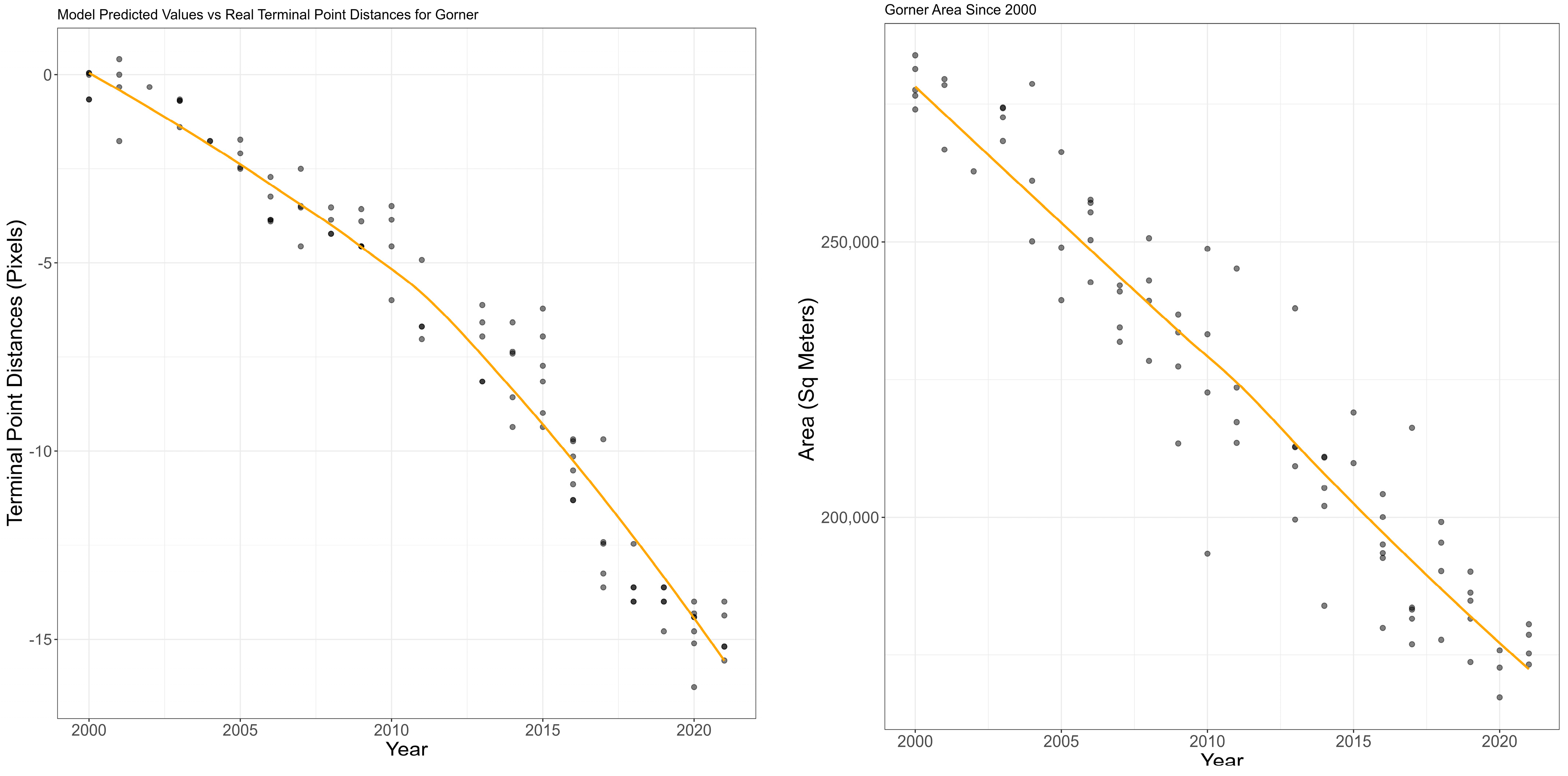
4.4. Variations in Gorner’s Terminal Point

Now that Franz Josef physical variations have been explained using general additive models, the following procedure will be done for Gorner glacier. The adjusted R 2 for the best multiple regression was 0.93 (Table 1c). Several general additive models were created taking into account different combination of climate factors. The best performing additive model was the linear combination of the smoothed function of monthly average maximum local temperature, precipitation and CO2 (Figure 11(Left)) with an adjusted R 2 of 0.94 and an AIC of 324 (Table 2c). A visual representation of the shapes of the smoothed function of the climate factors in the model can be seen in Appendix B. The confidence intervals for these three smoothed functions are narrow and closely follow the functions themselves, which indicate that the current function is performing accurately.
Both visual observation of predicted trend in Figure 11 and the adjusted R 2 for this model indicate that this model can robustly explain the variations of Gorner’s terminal point. To further confirm this, a comparison of the model’s output (yellow) for the variations of Gorner terminal point to the measured data (circles) is shown in Figure 11. As seen by a close look at the predicted trend in comparison with the measured data points, evidently the model performs well in explaining the glacier variation. Overall, the general additive model produced robust results for explaining the temporal glacier variations.

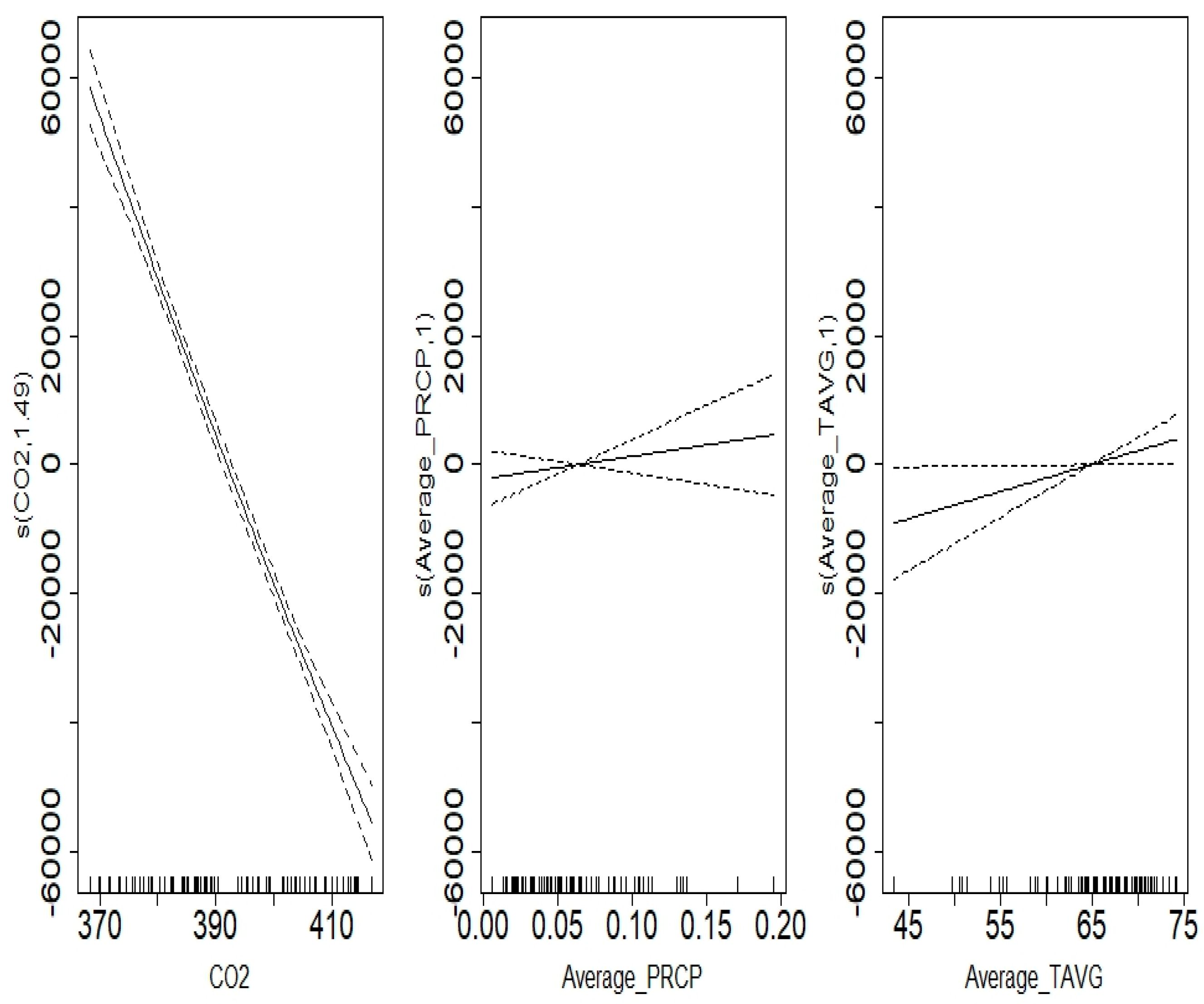
4.5. Variations in Gorner’s Area

Finally, we modeled the variations in the area of Gorner glacier. The best performing multiple regression model achieved an adjusted R 2 of 0.89. In comparison, the best performing generalized additive model for the changes in the area of Gorner glacier was a linear combination of the smoothed functions of monthly average of local temperature, precipitation, and CO2 (Figure 11(Right)). This model achieved an adjusted R 2 of 0.89 and an AIC of 1794 (Table 1d). It did not demonstrate an improvement in comparison with the best multiple regression model with the same adjusted R 2 of 0.89. However, GAM could better decipher the relation between the glacier variations and climate factors. The general additive model was comprised of three different smoothed function of climate factors, which can be seen in Appendix B. The smoothed functions provided robust model as seen by how close the confidence intervals (dashed lines) are to the actual smoothed functions. The model did have an adjusted R 2 of 0.89, so it can be indicated that the model produced promising results to explain the glacier variations.
By investigating different models in this study, it was concluded that GAM outperformed multiple regression in modeling temporal variations of the glacier’s terminal point and area. The proposed general additive models in this research were able to explain the variations fairly accurately using climate factors. Smoothed functions of temperature, local precipitation, and CO2 were identified as significant predictors in all implemented GAMs in this study, and it can be concluded that there is a strong relationship between the glacier’s temporal physical variations (for both Franz Josef and Gorner) and the climate factors.

5. Discussion

Two separate response variables representing glacier changes were quantified using Landsat imagery. First, spatial location of glacier terminus was traced over time as a proxy to glacier change. Second, glacier area was measured over time to quantify glacier variations. Response variables modeled using multiple regression and GAM. GAM could better model the nonlinear glacier variations. Global CO2 level, temperature (both local and global), and precipitation were identified as significant factors to model glacier variations. The results of this study agree with the previous research emphasizing the importance of local climate factors [17,18]. These finding are in line with what is currently known about the physics of glacier motion. The interaction between the climate factors could impact the glacier changes and potentially may help to better understand the complex dynamics of global climate subtleties.
As a proxy, spatiotemporal variation of glacier’s terminal point, offers valuable insights about glacier change. However, terminus variations do not provide sensible quantification of changes in the glacier’s size. Hence, quantification of glacier surface area by the proposed approach in this paper, provides essential insights about glacier’s size by measuring its surface area, in comparison with the previous works measuring terminus variations such as [19,20,21,22,23,24,25,26].
Moreover, due to the non-linear trends in the glacier variations, GAM could substantially improve the modeling of glacier’s variation using climate factors. The relation between glacier change and climate factors cannot be deciphered by linear models such as multiple regression. Hence, by the additional flexibility of a nonparametric approach, GAM could discover the nonlinear trends in the glacier variations that could not be inferred using linear models in the previous works [7,8,9].
Although the proposed semi-automated image segmentation pipeline is a promising approach, it still requires user’s input to customize it for different glaciers as distribution of pixel intensities changes in different scenes and over different spectral bands. This can prevent broad application to a large number of glaciers. Nevertheless, this study provides some proof of concept and valuable insights about complexity of this challenging problem. The segmentation can possibly be improved by the inclusion of processed bands using fusion of multiple Landsat spectral bands. Moreover, the computational cost of the entire process demands for an efficient data cleaning process in the preprocessing phase. Considering the scale and coverage of Landsat imagery along with the large number of glaciers around the globe, the clean-up process is not a trivial task.

6. Conclusions

Human communities rely on glaciers for water supply, agriculture, and drinking water. Rising temperatures due to the climate change cause mountain glaciers to melt and changes the water availability. Hence, modeling glacier variations in response to climate change is a pressing issue. Given that each glacier system is likely to be distinct both in the climate variations that it has experienced and in its response to these variations, a generic model may not be pertinent to model spatiotemporal variations of different glaciers. Moreover, historical measures of surface area or terminus location is essential to predict future spatiotemporal variations of glaciers. However, direct ground measurement is not feasible due to the remote nature of glaciers. Satellite imagery provides a practical approach to measure glacier area or to locate glacier terminus over time through remote sensing.
This work is in continuation of our previous works and is motivated by expedited recession of many glaciers around the globe while there is not a readily automated or semi-automated system available to quantify variations of a large number of mountain glaciers. In this work, a semi-automated pipeline was introduced to quantify glaciers in multispectral Landsat imagery. Data are gathered as a time sequence of spatially registered multispectral satellite imagery. The geometry of individual glaciers has been obtained using various image processing techniques including supervised classification, edge detection, and region segmentation. Then, two supervised learning methods including a parametric method (multiple regression) and a nonparametric method (generalized additive model) were implemented to identify climate factors that can impact glacier changes. This model can be customized for individual glaciers as the terminus position or surface area of individual glacier systems depend strongly on local basin geometry and local variations in temperature and precipitation. There are limiting factors to the accuracy of the predicted response including the resolution of satellite imagery, the visibility of the glacier in the images, the frequency of imaging, and the signal to noise ratio of satellite sensors. Several factors contribute to partial loss of contrast and variability in the quantified response value. Among them, some can be visually recognized such as the clouds and mountain shades. But some others are more intangible such as debris atop glacial ice, snow, and variations in humidity.

Author Contributions

Conceptualization, E.R., T.T.H., J.W. and N.N.K.; methodology, E.R., T.T.H., J.W. and N.N.K.; software, E.R., T.T.H., J.W. and N.N.K.; validation, E.R. and N.N.K.; formal analysis, E.R., T.T.H. and N.N.K.; investigation, E.R., T.T.H., J.W. and N.N.K.; resources, N.N.K.; data curation, E.R., T.T.H., J.W. and N.N.K.; writing—original draft preparation, E.R., T.T.H., J.W. and N.N.K.; writing—review and editing, E.R. and N.N.K.; visualization, E.R., T.T.H., J.W. and N.N.K.; supervision, N.N.K.; project administration, N.N.K.; funding acquisition, N.N.K. All authors have read and agreed to the published version of the manuscript.

Funding

This work was done as part of a REU (Research Experiences for Undergraduates) Statistical Models with Applications to Geoscience awarded by NSF (Grant # 1950768).

Data Availability Statement

MATLAB and R code is available upon reasonable request.

Conflicts of Interest

Authors declare no competing interest.

Appendix A

GAM Summary Tables
Gorner Area GAM
Area ~ s(Average_TAVG) + s(CO2) + s(Average_PRCP) + s(Global_Mean)
Parametric coefficients:EstimateStd ErrorT valuePr (>|T|)
Intercept225,4841279176.32.00 × 10−16
Smooth Termsedfref defFp-Value
s(Average_TAVG)113.1140.0817
s(CO2)1.1861.34796.12.00 × 10−16
s(Average_PRCP)110.4190.5194
s(Global_Mean)114.9440.0292
ModelAICDevianceAdj R2
1706.99689.388.7
Area ~ s(Average_TMAX) + s(CO2) + s(Average_PRCP) + s(Global_Mean)
Parametric coefficients:EstimateStd ErrorT valuePr (>|T|)
Intercept225,4841279176.32.00 × 10−16
Smooth Termsedfref defFp-Value
s(Average_TMAX)112.8660.0935
s(CO2)1.2951.52583.0512.00 × 10−16
s(Average_PRCP)110.5620.4555
s(Global_Mean)115.0840.0271
ModelAICDevianceAdj R2
1707.22389.388.7
Area ~ s(Average_TMIN) + s(CO2) + s(Average_PRCP) + s(Global_Mean)
Parametric coefficients:EstimateStd ErrorT valuePr (>|T|)
Intercept225,4841285175.52.00 × 10−16
Smooth Termsedfref defFp-Value
s(Average_TMIN)112.0940.1521
s(CO2)1.3271.57678.7222.00 × 10−16
s(Average_PRCP)110.3470.5578
s(Global_Mean)115.3530.0235
ModelAICDevianceAdj R2
1708.02989.288.6
Area ~ s(Average_TAVG) + s(CO2) + s(Global_Mean)
Parametric coefficients:EstimateStd ErrorT valuePr (>|T|)
Intercept225,4841273177.22.00 × 10−16
Smooth Termsedfref defFp-Value
s(Average_TAVG)113.730.0572
s(CO2)1.2671.46387.0252.00 × 10−16
s(Global_Mean)115.2920.0241
ModelAICDevianceAdj R2
1705.02989.288.8
Area ~ s(CO2) + s(Global_Mean)
Parametric coefficients:EstimateStd ErrorT valuePr (>|T|)
Intercept225,4841287175.32.00 × 10−16
Smooth Termsedfref defFp-Value
s(CO2)1.6481.87668.222.00 × 10−16
s(Global_Mean)119.240.00324
ModelAICDevianceAdj R2
1706.64388.988.5
Area ~ s(CO2) + s(Average_PRCP) + s(Global_Mean)
Parametric coefficients:EstimateStd ErrorT valuePr (>|T|)
Intercept225,4841286175.42.00 × 10−16
Smooth Termsedfref defFp-Value
s(Average_PRCP)1.1181.2221.0930.35734
s(CO2)1.6151.85269.4932.00 × 10−16
s(Global_Mean)118.0220.00591
ModelAICDevianceAdj R2
1707.75989.188.5
Gorner Area GAM
Area ~ s(CO2) + s(Average_PRCP) + s(Average_TAVG)
Parametric coefficients:EstimateStd ErrorT valuePr (>|T|)
Intercept223,1441262176.82.00 × 10−16
Smooth Termsedfref defFp-Value
s(Average_PRCP)110.9890.3232
s(CO2)1.4921.742364.2482.00 × 10−16
s(Average_TAVG)114.3560.0401
ModelAICDevianceAdj R2
1794.75989.488.9
Area ~ s(Global_Mean) + s(Average_PRCP) + s(Average_TAVG)
Parametric coefficients:EstimateStd ErrorT valuePr (>|T|)
Intercept225,4853150104.92.00 × 10−16
Smooth Termsedfref defFp-Value
s(Average_PRCP)110.0650.8
s(Global_Mean)11165.5232.00 × 10−16
s(Average_TAVG)111.1250.292
ModelAICDevianceAdj R2
1787.6569.268
Gorner Terminal Point Distance GAM
Distance ~ s(Average_TMIN) + s(CO2) + s(Average_PRCP) + s(Global_Mean)
Parametric coefficients:EstimateStd ErrorT valuePr (>|T|)
Intercept−6.91790.1306−52.962.00 × 10−16
Smooth Termsedfref defFp-Value
s(Average_TMIN)1.4851.8180.6230.616
s(CO2)2.5032.823111.8732.00 × 10−16
s(Average_PRCP)110.0370.848
s(Global_Mean)2.212.5980.8790.535
ModelAICDevianceAdj R2
310.161793.993.4
Distance ~ s(Average_TMAX) + s(CO2) + s(Average_PRCP) + s(Global_Mean)
Parametric coefficients:EstimateStd ErrorT valuePr (>|T|)
Intercept−6.91790.1306−52.982.00 × 10−16
Smooth Termsedfref defFp-Value
s(Average_TMAX)111.5420.218
s(CO2)2.5322.842114.9372.00 × 10−16
s(Average_PRCP)11.0010.0430.838
s(Global_Mean)2.0552.4560.6610.67
ModelAICDevianceAdj R2
308.907893.493.9
Distance ~ s(Average_TAVG) + s(CO2) + s(Average_PRCP) + s(Global_Mean)
Parametric coefficients:EstimateStd ErrorT valuePr (>|T|)
Intercept−6.91790.1308−52.92.00 × 10−16
Smooth Termsedfref defFp-Value
s(Average_TAVG)1.0011.0021.1730.282
s(CO2)2.5282.84113.3042.00 × 10−16
s(Average_PRCP)110.0270.871
s(Global_Mean)2.0972.960.7210.635
ModelAICDevianceAdj R2
309.216593.993.4
Distance ~ s(CO2) + s(Global_Mean)
Parametric coefficients:EstimateStd ErrorT valuePr (>|T|)
Intercept-6.91790.1319−52.442.00 × 10−16
Smooth Termsedfref defFp-Value
s(CO2)1.9381.996190.1092.00 × 10−16
s(Global_Mean)110.8780.351
ModelAICDevianceAdj R2
306.055893.593.3
Distance ~ s(CO2) + s(Average_PRCP) + s(Global_Mean)
Parametric coefficients:EstimateStd ErrorT valuePr (>|T|)
Intercept−6.91790.1325−52.22.00 × 10−16
Smooth Termsedfref defFp-Value
s(CO2)1.9381.996185.6692.00 × 10−16
s(Average_PRCP)110.1820.67
s(Global_Mean)110.7130.401
ModelAICDevianceAdj R2
307.84693.593.2
Gorner Terminal Point Distance GAM
Distance ~ s(CO2) + s(Average_PRCP) + s(Average_TMAX)
Parametric coefficients:EstimateStd ErrorT valuePr (>|T|)
Intercept−7.33180.1289−56.872.00 × 10−16
Smooth Termsedfref defFp-Value
s(Average_TMAX)111.9080.17
s(CO2)1.9331.995701.2552.00 × 10−16
s(Average_PRCP)110.1320.717
ModelAICDevianceAdj R2
324.239493.7
Distance ~ s(Global_Mean,) + s(Average_PRCP) + s(Average_TMAX)
Parametric coefficients:EstimateStd ErrorT valuePr (>|T|)
Intercept−6.91790.2971−23.292.00 × 10−16
Smooth Termsedfref defFp-Value
s(Average_TMAX)115.180.0253
s(Average_PRCP)110.5420.4636
s(Global_Mean)11176.0892.00 × 10−16
ModelAICDevianceAdj R2
453.73156765.9
Franz Josef Area GAM
Area ~ s(Average_TMIN) + s(CO2) + s(Average_PRCP) + s(Global_Mean)
Parametric coefficients:EstimateStd ErrorT valuePr (>|T|)
Intercept32126450.192.00 × 10−16
Smooth Termsedfref defFp-Value
s(Average_TMIN)110.2950.5929
s(CO2)2.4422.7742.55 × 10−2
s(Average_PRCP)113.6040.0721
s(Global_Mean)112.5080.1289
ModelAICDevianceAdj R2
382.896264.554.7
Franz Josef Area GAM
Area ~ s(Average_TMAX) + s(CO2) + s(Average_PRCP) + s(Global_Mean)
Parametric coefficients:EstimateStd ErrorT valuePr (>|T|)
Intercept3211.9658.7754.652.00 × 10−16
Smooth Termsedfref defFp-Value
s(Average_TMAX)1.9882.41.6710.186
s(CO2)2.3112.65446.33 × 10−2
s(Average_PRCP)1.3631.6071.1670.2345
s(Global_Mean)116.2320.0224
ModelAICDevianceAdj R2
380.574371.961.8
Area ~ s(Average_TMAX) + s(CO2) + s(Average_PRCP) + s(Global_Mean)
Parametric coefficients:EstimateStd ErrorT valuePr (>|T|)
Intercept3211.9664.3349.932.00 × 10−16
Smooth Termsedfref defFp-Value
s(Average_TAVG)110.110.7441
s(CO2)2.4332.76342.94 × 10−2
s(Average_PRCP)113.3630.0816
s(Global_Mean)112.2640.148
ModelAICDevianceAdj R2
383.161464.154.2
Area ~ s(Average_TMAX) + s(CO2) + s(Average_PRCP)
Parametric coefficients:EstimateStd ErrorT valuePr (>|T|)
Intercept3211.9670.7145.422.00 × 10−16
Smooth Termsedfref defFp-Value
s(Average_TMAX)110.0490.82713
s(CO2)1.9221.994101.08 × 10−3
s(Average_PRCP)111.4660.23938
ModelAICDevianceAdj R2
386.47553.344.6
Area ~ s(CO2) + s(Average_PRCP)
Parametric coefficients:EstimateStd ErrorT valuePr (>|T|)
Intercept3211.9669.1446.452.00 × 10−16
Smooth Termsedfref defFp-Value
s(CO2)1.9271.995117.85 × 104
s(Average_PRCP)111.770.196995
ModelAICDevianceAdj R2
384.509653.347.1
Area ~ s(Global_Mean) + s(CO2) + s(Average_PRCP)
Parametric coefficients:EstimateStd ErrorT valuePr (>|T|)
Intercept3211.9664.5849.732.00 × 10−16
Smooth Termsedfref defFp-Value
s(Global_Mean)114.4960.046
s(CO2)1.9051.99151.92 × 10−2
s(Average_PRCP)1.2091.3742.9410.1213
ModelAICDevianceAdj R2
382.266361.453.8
Franz Josef Terminal Point Distance GAM
Distance ~ s(Average_TMIN) + s(CO2) + s(Average_PRCP) + s(Global_Mean)
Parametric coefficients:EstimateStd ErrorT valuePr (>|T|)
Intercept-5.48940.3898−14.12.00 × 10−16
Smooth Termsedfref defFp-Value
s(Average_TMIN)1.2741.493.4560.073
s(CO2)2.8682.98747.0242.00 × 10−16
s(Average_PRCP)110.0460.8303
s(Global_Mean)115.4290.0223
ModelAICDevianceAdj R2
480.79986.185
Distance ~ s(CO2) + s(Global_Mean)
Parametric coefficients:EstimateStd ErrorT valuePr (>|T|)
Intercept−5.26720.3834−13.742.00 × 10−16
Smooth Termsedfref defFp-Value
s(CO2)1.991274.2922.00 × 10−16
s(Global_Mean)1.251.4373.9050.0283
ModelAICDevianceAdj R2
500.76684.984.3
Distance ~ s(Average_TMIN) + s(CO2) + s(Global_Mean)
Parametric coefficients:EstimateStd ErrorT valuePr (>|T|)
Intercept−5.26720.3738−14.092.00 × 10−16
Smooth Termsedfref defFp-Value
s(Average_TMIN)1.2081.3723.6620.0336
s(CO2)1.991275.3182.00 × 10−16
s(Global_Mean)115.5750.0204
ModelAICDevianceAdj R2
497.056885.885.1
Distance ~ s(CO2) + s(Average_PRCP) + s(Global_Mean)
Parametric coefficients:EstimateStd ErrorT valuePr (>|T|)
Intercept−5.48940.3984−13.782.00 × 10−16
Smooth Termsedfref defFp-Value
s(CO2)1.991.99970.4182.00 × 10−16
s(Average_PRCP)110.0860.7705
s(Global_Mean)1.3541.5822.680.0608
ModelAICDevianceAdj R2
482.936985.184.3
Distance ~ s(CO2) + s(Average_PRCP) + s(Average_TMIN)
Parametric coefficients:EstimateStd ErrorT valuePr (>|T|)
Intercept−5.72410.3942−14.522.00 × 10−16
Smooth Termsedfref defFp-Value
s(Average_TMIN)1.4711.7212.9720.0414
s(CO2)22225.6292.00 × 10−16
s(Average_PRCP)110.0010.9839
ModelAICDevianceAdj R2
487.699785.985.1

Appendix B

Modeling Franz Josef TerminusAlgorithms 16 00486 i001
Modeling Franz Josef AreaAlgorithms 16 00486 i002
Modeling Gorner TerminusAlgorithms 16 00486 i003
Modeling Gorner AreaAlgorithms 16 00486 i004

References

  1. Bhattacharya, A.; Bolch, T.; Mukherjee, K.; King, O.; Menounos, B.; Kapitsa, V.; Neckel, N.; Yang, W.; Yao, T. High Mountain Asian glacier response to climate revealed by multi-temporal satellite observations since the 1960s. Nat. Commun. 2021, 12, 4133. [Google Scholar] [CrossRef] [PubMed]
  2. Bolivia’s Tuni Glacier Is Disappearing, and So Is the Water It Supplies. Reuters. 2021. Available online: https://www.reuters.com/article/us-bolivia-environment-glacier/bolivias-tuni-glacier-is-disappearing-and-so-is-the-water-it-supplies-idUSKBN29929U (accessed on 20 October 2022).
  3. Laghari, J. Climate change: Melting glaciers bring energy uncertainty. Nature 2013, 502, 617–618. [Google Scholar] [CrossRef] [PubMed]
  4. GLIMS; NSIDC. Global Land Ice Measurements from Space Glacier Database; International GLIMS Community and the National Snow and Ice Data Center: Boulder, CO, USA, 2005; updated 2018. [Google Scholar] [CrossRef]
  5. Raup, B.; Racoviteanu, A.; Khalsa, S.J.; Helm, C.; Armstrong, R.; Arnaud, Y. The GLIMS geospatial glacier database: A new tool for studying glacier change. Glob. Planet. Chang. 2007, 56, 101–110. [Google Scholar] [CrossRef]
  6. Chen, L.; Zhang, W.; Yi, Y.; Zhang, Z.; Chao, S. Long time-series glacier outlines in the three-rivers headwater region from 1986 to 2021 based on deep learning. IEEE J. Sel. Top. Appl. Earth Obs. Remote Sens. 2022, 15, 5734–5752. [Google Scholar] [CrossRef]
  7. Kachouie, N.N.; Gerke, T.; Huybers, P.; Schwartzman, A. Nonparametric regression for estimation of spatiotemporal mountain glacier retreat from satellite images. IEEE Trans. Geosci. Remote Sens. 2014, 53, 1135–1149. [Google Scholar] [CrossRef]
  8. Kachouie, N.N.; Huybers, P.; Schwartzman, A. Localization of mountain glacier termini in Landsat multi-spectral images. Pattern Recognit. Lett. 2013, 34, 94–106. [Google Scholar] [CrossRef]
  9. Onyejekwe, O.; Holman, B.; Kachouie, N.N. Multivariate models for predicting glacier termini. Environ. Earth Sci. 2017, 76, 807. [Google Scholar] [CrossRef]
  10. Lea, J.M.; Mair, D.W.; Rea, B.R. Evaluation of existing and new methods of tracking glacier terminus change. J. Glaciol. 2014, 60, 323–332. [Google Scholar] [CrossRef]
  11. Landsat 8 Data Users, Handbook|U.S. Geological Survey. Available online: https://www.usgs.gov/landsat-missions/landsat-8-data-users-handbook (accessed on 9 October 2023).
  12. Hastie, T.; Tibshirani, R. Generalized Additive Models. Stat. Sci. 1986, 1, 297–310. Available online: https://www.jstor.org/stable/2245459 (accessed on 9 October 2023). [CrossRef]
  13. Marra, G.; Wood, S.N. Practical variable selection for generalized additive models. Comput. Stat. Data Anal. 2011, 55, 2372–2387. [Google Scholar] [CrossRef]
  14. Wood, S.N. Generalized Additive Models: An Introduction with R; CRC Press: Boca Raton, FL, USA, 2017. [Google Scholar]
  15. Nychka, D. Bayesian confidence intervals for smoothing splines. J. Am. Stat. Assoc. 1988, 83, 1134–1143. [Google Scholar] [CrossRef]
  16. Patterson, H.D.; Thompson, R. Recovery of inter-block information when block sizes are unequal. Biometrika 1971, 58, 545–554. [Google Scholar] [CrossRef]
  17. Sutton, R.; Suckling, E.; Hawkins, E. What Does Global Mean Temperature Tell Us about Local Climate? Philos. Trans. R. Soc. A 2015, 373, 20140426. [Google Scholar] [CrossRef] [PubMed]
  18. Hooke, R.L. Principles of Glacier Mechanics; Cambridge University Press: Cambridge, UK, 2019. [Google Scholar]
  19. Moon, T.; Joughin, I. Changes in ice front position on Greenland’s outlet glaciers from 1992 to 2007. J. Geophys. Res. Earth Surf. 2008, 113. [Google Scholar] [CrossRef]
  20. Cuffey, K.M.; Paterson, W.S. The Physics of Glaciers; Academic Press: Cambridge, MA, USA, 2010. [Google Scholar]
  21. Robson, B.A.; Bolch, T.; MacDonell, S.; Hölbling, D.; Rastner, P.; Schaffer, N. Automated detection of rock glaciers using deep learning and object-based image analysis. Remote Sens. Environ. 2020, 250, 112033. [Google Scholar] [CrossRef]
  22. Ren, J.; Jing, Z.; Pu, J.; Qin, X. Glacier variations and climate change in the central Himalaya over the past few decades. Ann. Glaciol. 2006, 43, 218–222. [Google Scholar] [CrossRef]
  23. Lovell, A.M.; Stokes, C.R.; Jamieson, S.S. Sub-decadal variations in outlet glacier terminus positions in Victoria Land, Oates Land and George V Land, East Antarctica (1972–2013). Antarct. Sci. 2017, 29, 468–483. [Google Scholar] [CrossRef]
  24. Schild, K.M.; Hamilton, G.S. Seasonal variations of outlet glacier terminus position in Greenland. J. Glaciol. 2013, 59, 759–770. [Google Scholar] [CrossRef]
  25. Meng, Q.; Chen, X.; Huang, X.; Huang, Y.; Peng, Y.; Zhang, Y.; Zhen, J. Monitoring glacier terminus and surface velocity changes over different time scales using massive imagery analysis and offset tracking at the Hoh Xil World Heritage Site, Qinghai-Tibet Plateau. Int. J. Appl. Earth Obs. Geoinf. 2022, 112, 102913. [Google Scholar] [CrossRef]
  26. Yang, R.; Hock, R.; Kang, S.; Guo, W.; Shangguan, D.; Jiang, Z.; Zhang, Q. Glacier surface speed variations on the Kenai Peninsula, Alaska, 2014–2019. J. Geophys. Res. Earth Surf. 2022, 127, e2022JF006599. [Google Scholar] [CrossRef]
Figure 1. Regional Glacier Network Overview.
Algorithms 16 00486 g001
Figure 2. (Left panel) Illustrative Terminal point identification methods. Top: (left) Center-Line method; (middle) Bow method (right) Rectilinear Box method. Bottom: (left) Curvilinear Box method; (right) Extrapolated Center-Line method. (Right panel) Illustrative Terminal point tracking method.
Algorithms 16 00486 g002
Figure 3. Glaciers of Interest. Left: Gorner. Right: Franz Josef.
Algorithms 16 00486 g003
Figure 4. Example of Landsat images removed from dataset shown in false colors. Cloudy and invisible (Left); Covered by mountain shadow (Middle); Sensor malfunction (Right).
Algorithms 16 00486 g004
Figure 5. (Left) Multispectral band information for images taken by Landsat 7. (Middle) Top Franz Josef; Bottom: Gorner; from left to right: Band 1, Band 5, Band 6 shown in false colors. (Right) Terminal Identification process.
Algorithms 16 00486 g005
Figure 6. Schematic of Proposed Method.
Algorithms 16 00486 g006
Figure 7. (Left) Two scenes of the Franz Josef glacier superimposed (green, 1990; purple, 2009); (Right) Two scenes of the Gorner glacier superimposed (green, 1984; purple, 2009). Red arrows highlight the recession.
Algorithms 16 00486 g007
Figure 8. (Top) Time Series for the terminus variations 2000 to 2021 (pixel resolution is 30 meters). (Bottom) Time series for the area variations 2000 to 2021.
Algorithms 16 00486 g008
Figure 9. (Left) Generalized Additive Model for Franz Josef Terminus 2000 to 2009 (pixel resolution is 30 meters). (Right) Generalized Additive Model for Franz Josef Area 2000 to 2009. Measured (circles), trend (blue), and confidence interval (gray shade).
Algorithms 16 00486 g009
Figure 10. (Left) Generalized Additive Model for Franz Josef Terminus 2000 to 2021 (pixel resolution is 30 meters). (Right) Generalized Additive Model for Franz Josef Area 2000 to 2021. Measured (circles) and trend (yellow).
Algorithms 16 00486 g010
Figure 11. (Left) Generalized Additive Model for Gorner Terminus 2000 to 2021 (pixel resolution is 30 meters). (Right) Generalized Additive Model for Gorner Area 2000 to 2021. Measured (circles) and trend (yellow).
Algorithms 16 00486 g011
Table 1. Multiple Regression Models. (a) Terminal Point of Franz Josef as Response. (b) Area of Franz Josef as Response. (c) Terminal Point of Gorner as Response. (d) Area of Gorner as Response.
(a)
Franz Josef Terminal Point
Model Index Predictors
1CO2
2CO2 Global_Mean
3CO2 Average_TMAX Global_Mean
4Average_PRCP CO2 Average_TMAX Global_Mean
Subsets Regression
ModelR-SquareAdj. R-SquarePred. R-SquareC(p)AICSBICSBCMSEPFPEHSPAPC
10.580.570.5619.07599338607349538.820.430.44
20.640.630.611.93577319587287132.590.360.39
30.650.630.612.21577319590284732.650.360.39
40.650.640.615.00555308569277933.770.390.39
(b)
Franz Josef Area
Model Index Predictors
1Global_Mean
2Average_TMAX Global_Mean
3Average_PRCP Average_TMAX Global_Mean
4Average_PRCP CO2 Average_TMAX Global_Mean
Subsets Regression
ModelR-SquareAdj. R-SquarePred. R-SquareC(p)AICSBICSBCMSEPFPEHSPAPC
10.340.310.244.743893153934,213,050174,46070430.77
20.430.380.273.023873143923,792,603162,35166160.72
30.470.400.263.253873153933,667,00862,05266870.72
40.480.380.205.003893173963,805,281173,37472700.77
(c)
Gorner Terminal Point
Model Index Predictors
1CO2
2CO2 Average_TMAX
3Average_PRCP CO2 Average_TMAX
4Average_PRCP CO2 Average_TMAX Global_Mean
Subsets Regression
ModelR-SquareAdj. R-SquarePred. R-SquareC(p)AICSBICSBCMSEPFPEHSPAPC
10.930.930.93−2.00333613411741.850.01950.07
20.930.930.93−0.82334623441741.870.01970.07
30.930.930.931.18336643491761.910.02020.08
40.92 0.920.915.00323653381722.000.02230.09
(d)
Gorner Area
Model Index Predictors
1CO2
2CO2 Average_TMAX
3Average_PRCP CO2 Average_TMAX
4Average_PRCP CO2 Average_TMAX Global_Mean
Subsets Regression
ModelR-SquareAdj. R-SquarePred. R-SquareC(p)AICSBICSBCMSEPFPEHSPAPC
10.880.880.8810.517981562180511,904,380,369146,881,2581,792,8150.12
20.890.890.886.017941558180311,200,129,510139,795,8551,707,8380.12
30.890.890.886.717941559180611,145,284,672140,706,3261,720,9880.12
40.890.890.885.017061483172110,264,439,570138,078,1491,778,8930.12
Table 2. Generalized Additive: Models. (a) Terminal Point of Franz Josef as Response. (b) Area of Franz Josef as Response. (c) Terminal Point of Gorner as Response. (d) Area of Gorner as Response. Find the complete set of models in Appendix A.
(a)
Franz Josef Terminal Point Distance GAM
Distance ~ s(Average_TMIN) + s(CO2) + s(Average_PRCP) + s(Global_Mean)
Parametric coefficients:Estimate Std ErrorT valuePr (>|T|)
Intercept−5.48940.3898−14.12 × 10⁻¹⁶
Smooth Terms EDFREF DEFFp-Value
s(Average_TMIN) 1.2741.493.4560.073
s(CO2)2.8682.98747.0242 × 10−16
s(Average_PRCP) 110.0460.8303
s(Global_Mean) 115.4290.0223
ModelAIC Deviance Adj R2
480.79986.185
(b)
Franz Josef Area GAM
Area ~ s(Average_TMAX) + s(CO2) + s(Average_PRCP) + s(Global_Mean)
Parametric coefficients:Estimate Std ErrorT valuePr (>|T|)
Intercept3211.9658.7754.652 × 10−16
Smooth Terms EDFREF DEFFp-Value
s(Average_TMAX) 1.9882.41.6710.186
s(CO2)2.3112.65446.33 × 10−2
s(Average_PRCP) 1.3631.6071.1670.2345
s(Global_Mean) 116.2320.0224
ModelAIC Deviance Adj R2
380.574371.961.8
(c)
Gorner Terminal Point Distance GAM
Distance ~ s(CO2) + s(Average_PRCP) + s(Average_TMAX)
Parametric coefficients:Estimate Std ErrorT valuePr (>|T|)
Intercept−7.33180.1289−56.872 × 10⁻¹⁶
Smooth Terms EDFREF DEFFp-Value
s(Average_TMAX)111.9080.17
s(CO2)1.9331.995701.2552 × 10−16
s(Average_PRCP) 110.1320.717
ModelAIC Deviance Adj R2
324.239493.7
(d)
Gorner Area GAM
Area ~ s(CO2) + s(Average_PRCP) + s(Average_TAVG)
Parametric coefficients:Estimate Std ErrorT valuePr (>|T|)
Intercept223,1441262176.82 × 10−16
Smooth Terms EDFREF DEFFp-Value
s(Average_PRCP) 110.9890.3232
s(CO2)1.4921.742364.2482 × 10−16
s(Average_TAVG) 114.3560.0401
ModelAIC Deviance Adj R2
1794.75989.488.9
Disclaimer/Publisher’s Note: The statements, opinions and data contained in all publications are solely those of the individual author(s) and contributor(s) and not of MDPI and/or the editor(s). MDPI and/or the editor(s) disclaim responsibility for any injury to people or property resulting from any ideas, methods, instructions or products referred to in the content.

