Manifold Explorer: Satellite Image Labelling and Clustering Tool with Using Deep Convolutional Autoencoders

Abstract

We present a novel approach to providing greater insight into the characteristics of an unlabelled dataset, increasing the efficiency with which labelled datasets can be created. We leverage dimension-reduction techniques in combination with autoencoders to create an efficient feature representation for image tiles derived from remote sensing satellite imagery. The proposed methodology consists of two main stages. Firstly, an autoencoder network is utilised to reduce the high-dimensional image tile data into a compact and expressive latentfeature representation. Subsequently, features are further reduced to a two-dimensional embedding space using the manifold learning algorithm Uniform Manifold Approximation and Projection (UMAP) and t-distributed Stochastic Neighbour Embedding (t-SNE). This step enables the visualization of the image tile clusters in a 2D plot, providing an intuitive and interactive representation that can be used to aid rapid and geographically distributed image labelling. To facilitate the labelling process, our approach allows users to interact with the 2D visualization and label clusters based on their domain knowledge. In cases where certain classes are not effectively separated, users can re-apply dimension reduction to interactively refine subsets of clusters and achieve better class separation, enabling a comprehensively labelled dataset. We evaluate the proposed approach on real-world remote sensing satellite image datasets and demonstrate its effectiveness in achieving accurate and efficient image tile clustering and labelling. Users actively participate in the labelling process through our interactive approach, leading to enhanced relevance of the labelled data, by allowing domain experts to contribute their expertise and enrich the dataset for improved downstream analysis and applications.

1. Introduction

Rapid growth in remote sensing (RS) technologies and deployed satellite missions has led to substantially large remote sensing imagery datasets. A single remote sensing mission can have multiple different apparatuses that simultaneously and continuously collect data. For example, the Sentinel 2 satellite missions are comprised of two launched satellites (Sentinel 2A and 2B) collecting multi-spectral images, with the latter producing 1.6 terabytes of data per day. The diversity and complexity of RS data give validity and definition to the RS big data problem [1]. Many techniques used to explore and categorise these images for downstream analysis require previously labelled samples to be able to train and test algorithms on unseen imagery. Increasing the volume and diversity of labelled samples gives more confidence that we can attribute to any given algorithm as it has been tested on a more diverse sample range. However, acquiring a sufficiently large and accurately labelled dataset of images for any given RS technology and technique requires immense effort from an RS expert analyst [2].

Ultimately, this results in a significant problem of sorting data of interest from the ever-growing volume and diversity of image datasets. Producing labelled images for analysis requires a large effort from remote sensing specialists when considering temporal differences for one location, which is then compounded by involving multiple locations. Providing context to images by binning them into categories or labels from a human perspective is to understand the physical matter and contextual arrangement of pixels within an image. The physical matter of any individual pixel can be discerned by the reflected wavelengths of light detected by the studied imaging platform, e.g., for a red green and blue image, plant matter is green. Increasing the diversity of detected wavelengths from a simple RGB composite image can improve our understanding of materials, which is why modern satellite missions include infrared detection capabilities facilitating the use of hand-crafted feature extraction methods such as Normalized Difference Water Index (NDWI) [3] and Normalized Difference Vegetation Index (NDVI) [4]. However, such techniques ignore the geographical arrangement and contextual information within an image, as certain features are often located near each other, e.g., buildings and roads, mountains and tributaries, etc. [5]. Images that have the same physical matter or arrangement similar to a known sample will have a similar value from a hand-crafted feature. To discern whether the score is similar or not, techniques like K-means clustering, SVM, LDA or GMM’s are utilised [6,7]. Expanding these techniques to accommodate unseen samples or non-trivial problems could require clustering all old and new samples again, in addition to redefining the hand-crafted features to include the new subtleties within the data [8].

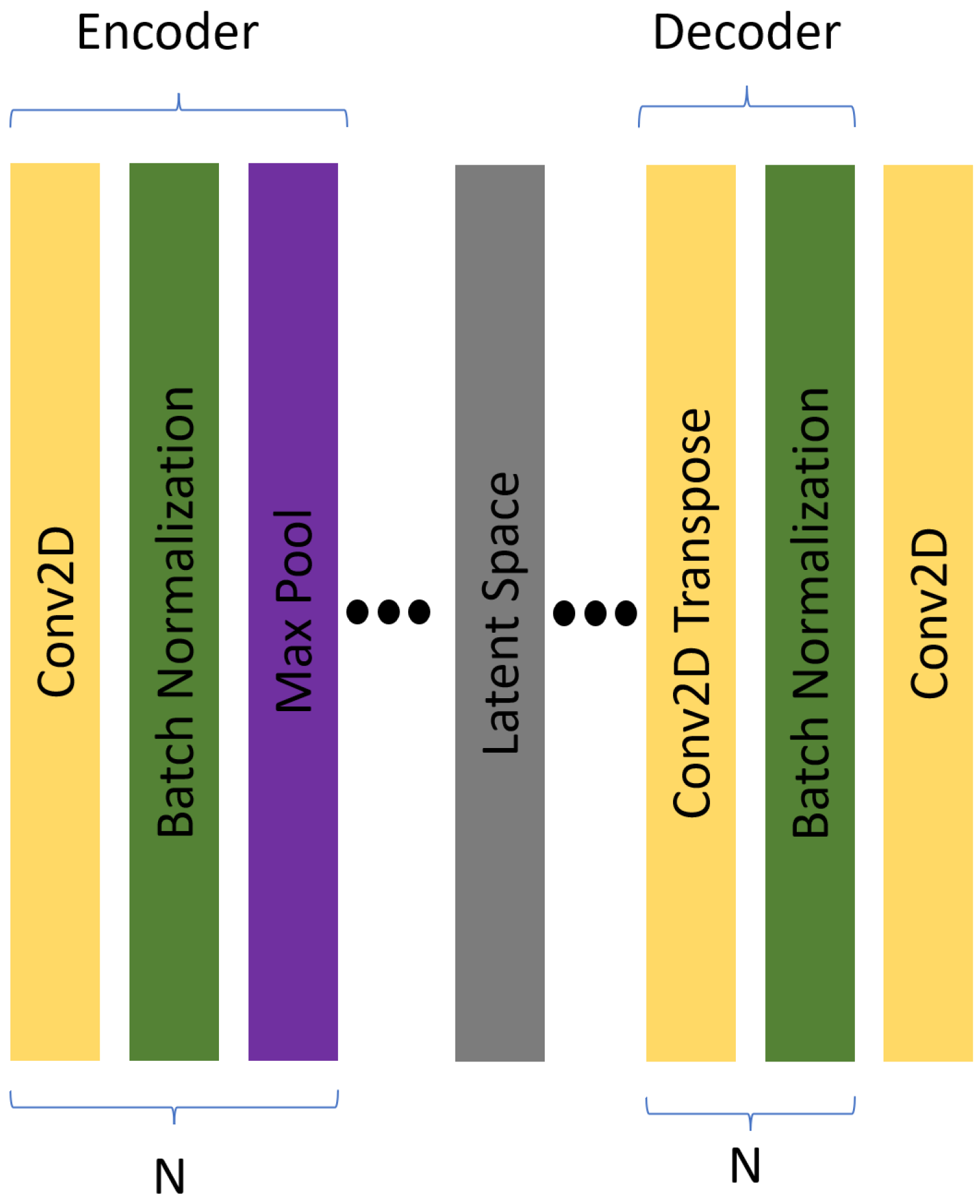
These hand-crafted features have in recent years been replaced by the use of deep convolutional neural network (DCNN) techniques. A DCNN produces optimised filters for the analysis of images based on the textures present creating complex non-linear representations. Building on Stacked Auto Encoders (SAE) [9] convolutional autoencoders add spatial learning abilities by introducing learnt filters and activation maps, allowing the model to learn local texture representations and inter-channel information. This architectural design for feature representation has demonstrated considerable success in remote sensing, as evidenced by various studies [10,11,12,13]. There are many variants of AEs that have also been utilised, such as Variational AEs (VAEs), that replace the latent space with a distribution instead that have been used in, for example, image captioning [14], desertification [15] or biomass prediction [16].

Querying images for similarity can be seen in the field of Image Retrieval (IR) within the RS field [17]. IR algorithms apply a form of top K retrieval, where K denotes the number of samples to be retrieved. Solutions for encoding functions within IR also utilise AE architectures for unsupervised feature extraction [18]. However, this approach limits the user to a variable number of images returned and requires an initial query image. In order to consider all images within a dataset there are further dimensionality reduction techniques that find manifolds of similar images. This approach has been considered with regard to time-series data [19,20] and time-series clustering [21].

Manifold projection involves mapping high-dimensional data into lower dimensions and can be formulated as attempting to keep pairwise distances as defined in the higher dimensional space as similar as possible to pairwise distances within the lower dimensional space, such as classical multi-dimensional scaling (MDS) [22]. Dimensions in this context refer to the number of variables representing the information. Different approaches to reduction may look to find low-dimensional representations of nonlinear manifolds or patterns in high-dimensional space [23]. For singular manifold representation, common algorithms include MDS, isometric mapping (ISOMAP), and locally linear neighbourhood (LLE) [24,25]. When considering multiple manifolds in high dimensional space, efficiency dictates comparing pairwise points in local space rather than the global pairwise distance between all points. A similarity matrix can be created that focuses on connecting similar neighbours and an assumption that many short paths (small geodesic distances) between points indicates these points are likely part of the same underlying structure in the data. Existing algorithms that do so for multiple manifolds include variations of ISOMAP, LLE, Hessian LLE or Laplacian Eigenmaps, each with varying suitability to certain tasks and limitations [26].

Stochastic Neighbourhood Embedding (SNE) computes the locality between points in a neighbourhood converting samples into probabilistic samples based on the Euclidean distance [27]. The low-dimensional embedding is created by enforcing the low-dimensional probabilities to be similar to the higher-dimensional embeddings. SNE proved capable of preserving local neighbourhoods in lower dimensional space; however, it suffered from many points overlapping in the projection, referred to as the crowding problem [28]. t-SNE was introduced to allow for effective visualization of multiple, related, high-dimensional manifolds by revealing structures at many different scales [29]. To overcome the crowding problem t-SNE was introduced where a long tail distribution was introduced to the lower dimensions, in contrast, the use of a heavy tail distribution has been shown to tighten clusters [29,30].

UMAP [31] is similar to t-SNE, in that both use gradient descent to optimize the embedding space. UMAP construction is based on a fuzzy graph approach of the high dimensional embedding in an attempt to accurately represent the topology. The low-dimensional embedding is then optimised to conform to the high-dimensional graphs and weights. UMAP aims to provide a more global context to the low-dimensional embedding comparatively to t-SNE, which can be attributed to the initialization of the low dimensional embedding space created by a fuzzy graph [32]. Many recent papers debate the similarities and differences between these two algorithms. In summary, both t-SNE and UMAP produce similar results when given similar initial conditions and both have been shown to be sensitive to starting parameters and low embedding [33].

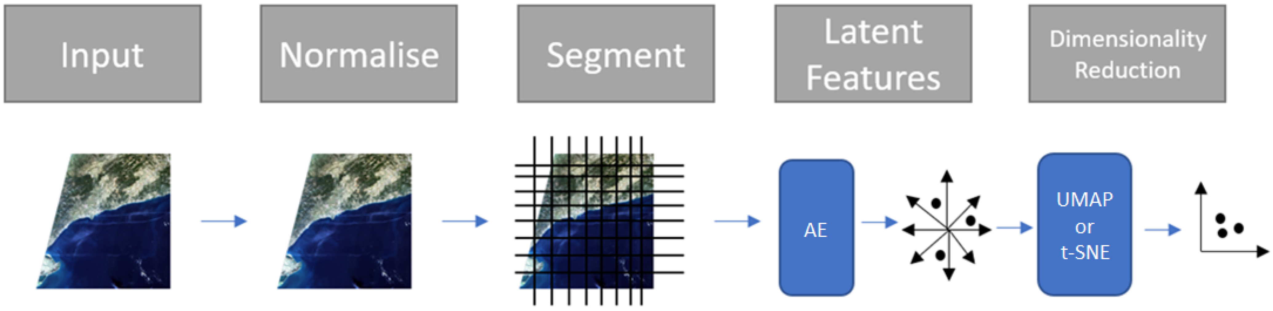
Our approach presents the user with a mass labelling interface enabling them to explore a dataset of satellite images. Class labels can be applied to multiple images at a time during user selection of those images in the interface. The classes are determined by the user and correspond to the visual features they want to extract, separate or label. Our interactive approach, utilising manifold projection, allows similar images to be selected simultaneously, which aids labelling. The use of visualisation techniques highlights different geographical features within images and how they relate to the trained filters of a CNN. Any complex dataset results in a lossy representation for both AI models and manifold projection, when regarding all features and variations, hindering a user from simply selecting and labelling large volumes of data with ease. As models require considerable time for training, we look to reduce the impact of information lost in manifold projection by utilising interactive visualisations. By allowing the user to interact with how these projections work, they can control and tease out better class separation from their fixed model, thus enabling a greater labelling throughput. This is discussed in more detail with examples in the next sections.

2. Materials and Methods

2.1. Materials

We use the public Sentinel 2 water edges dataset (SWED) [34], which contains multiple coastal geographic locations, comprised of 16 labelled $\mathrm{10,980}\times \mathrm{10,980}$ tiles (the large Sentinel 2 images are known as tiles). The images were selected to have minimal coverage of clouds with no preprocessing apart from bottom-of-atmosphere correction [35]. This dataset is rich in contrast and variety of physical coastal features in each geographical location with the addition of multiple fine-grained physical features such as jetties and bridges. The hypothesis is that we can see the transition of features and the evolution of the manifold with respect to both small features and larger geographical changes. Including water and land also introduces the complexity of the feature transition between both. Most papers within the domain of satellite imagery utilise datasets that are geographical location- or feature-specific as also expressed by the authors of the SWED dataset [34] who also find that water and coastline mapping is restricted to singular regions in the literature as one of their motivations to publish a dataset rich in variety. As the dataset contains a wide range of features, we can also explore the relationship of geographical features and their similarity in regards to how a CNN differentiates them. The atmospheric conditions around the world drastically change the reflection intensity recorded by a satellite for similar features.

2.2. Methods

We use the pipeline as depicted in Figure 1 where after pre-processing, we train an autoencoder to provide the latent features on which we apply dimension reduction to produce an embedding space that supports an interactive user interface.

2.2.1. Preprocessing

Each tile extracted from a Sentinel 2 product is $\mathrm{10,980}\times \mathrm{10,980}$ at 10 m resolution, meaning each pixel represents 10 m${}^2$ of the Earth’s surface area. We divide each image into 256 by 256 patches to balance computational efficiency and local feature representation. As we do not utilise a sliding window approach, there is a remainder of 228 discarded pixels along the right and bottom border. Opting for smaller patch sizes could increase the performance of the AE as fewer geographic features are present. While relatively large, the selection of patch size encapsulates enough local context to be discernible without the need to reference neighbouring patches and achieves a good visual representation within the final visualisation tool. The final dataset comprises 1764 images for each tile and a total of 28,224 images across all 16 locations. Sentinel 2 products are recorded in 13 different wavelengths all at varying spatial resolution. In our analysis, we focused exclusively on the red, green, blue, and near-infrared bands as they all record in the highest spatial resolution of 10 m.

2.2.2. Autoencoder Architecture

Each encoder within this architecture consists of a convolutional layer followed by batch normalisation, and max-pooling. Stacking these encoder blocks together forms a Stacked Autoencoder (SAE). The convolutional layers use a 3 × 3 kernel and ReLU for activation. At the end of the encoder is a dense layer for the conversion of feature maps to vectors enabling extraction of the latent space variables. The decoder combines up-sampling within the convolutional layer. The decoder is mirrored in the number of, N, units stacked to create the full decoder allowing the network to generate high-resolution feature maps, see Figure 2. The encoder and decoder are independent models and therefore share no information apart from the loss incurred during reconstruction whilst training.

The encoder consists of 5 blocks. The initial layer starts with 256 filters, halving for each subsequent layer. Each max-pooling layer scales the image by a factor of 2. The latent space, represented by the dense layer, has 1024 units. Training data are categorized into 10 groups based on the water content in each image, where to handle the significant difference in reflectance between water and land features, we weight the training batches based on the water content. We calculate the water content using the McFeeters Normalized Difference Water Index (NDWI) [36], which measures the difference between the green and near-infrared bands. As we aim to introduce an unsupervised pipeline we chose to not utilise the labels for water in the SWED dataset. The difference between ground truth and NDWI labels when binned was similar apart from noise introduced by clouds. The model is trained on mostly land content and validated on a set equally balanced between water and land. Data augmentation adds further variation using rotated images and adding salt and pepper noise, adjusting random pixels either to 0 or 1, to improve model generalisation. The optimal point in training is reached when the test loss matches the validation loss for 10 epochs, with the validation loss typically being lower due to more uniform textural information being present in water. The latent space vector provided by the autoencoder of size 1024 is passed on to subsequent stages of our pipeline.

2.2.3. Dimensionality Reduction

Further dimensionality reduction to two-dimensional embedding space is conducted with respect to the latent space produced by the autoencoder using t-SNE and UMAP. We chose two dimensions for simplicity and ease of downstream visualisation and interaction [37]. We use the Barnes–Hut approximation of t-SNE for its much faster computational advantages [38]. In addition, we implemented the algorithm with variable tail distribution in low dimensions to both overcome the overcrowding problem and the ability to make it heavy-tailed for tighter clusters. Our implementation enables user interaction with the number of iterations and to replay iterations by recording each iteration’s variables. The user can navigate between optimisation steps for any patterns that are presented earlier [39]. Data can be labelled at any optimisation step, with those labels then available to previous and future iterations. The first process of t-SNE is to optimise the embeddings with a lower learning rate and once it achieves an embedding that does not change for a few iterations, variable on data content and size, the learning rate is increased to expand and optimise the embedding. Visualising earlier iterations of t-SNE would allow a user to explore any emerging clusters without needing to wait for the finished process. As time complexity increases with dataset size earlier iterations may provide expedient clusters to the user. Finally, we added the ability to change the perplexity parameter of t-SNE for the user to assign depending on if they require more global or local attention. We defined a custom version of t-SNE based on existing libraries for implementation. The resulting Python scripts are embedded into our application.

We do not make any changes to UMAP and therefore refer to the original paper for the implementation [31]. We do however allow the user to input parameters such as minimum distance and the N nearest neighbours that UMAP should compute. Both parameters govern how the initial fuzzy graph is computed by UMAP and therefore can change the visualisation and its ability to show coherent clusters or manifolds.

2.2.4. Visualisation

Figure 3 presents the graphical UI for exploring the data and applying class labels to the satellite tiles. The main feature (D) is the two-dimensional embedding of the data in the form of a scatter plot. A content browser (F) displays the 256 by 256 image patch associated with each point. A map view (E) plots the location of each tile. Other windows (A–C) display, respectively, the data set explorer, t-SNE parameter interaction (in this case) and the class labels.

After a data set has been chosen the initial view is displayed. For each dataset embedding, there are two forms of visualizations presented to the user, UMAP or t-SNE, each can be navigated from Manifold Explorer. Each embedding in the two-dimensional scatter plot shows with respect to the reduction technique the manifolds and patterns within the high-dimensional space for the dataset provided. Points between clusters or within a line show the transition between similar images as the features evolve for the particular manifold. For t-SNE embeddings, we included the ability for the user to customize the parameter and iterations displayed within its own contained user interface. Each embedding is accessed by interacting with a slider to swap between each iteration.

The ability to zoom and filter regions of interest is implemented with a box selection method. The box can be drawn to any size and translated on the x, and y-axis by dragging. As points are selected, the content browser and map are updated. As all images are georeferenced, the map will have a small red marker in the geographical location of all selected samples for added context to labelling decisions. The content browser also updates to show an RGB composite of the selected images, which is how the user understands the contents of the manifold. Given the small pixel resolution of satellite images, we also included two sliders to change the image size and padding between samples.

Labelling is also conducted through the selection box. Selecting scatter points and pressing a number will label all points to the respective label. Selecting an image in the content browser will display a sub-menu where the user can select the label for the specific image.

We also implement an analogy of version control where a dataset can be branched into multiple subsets, each in a sand-boxed environment consisting of the same interface. The user can explore and label the subset and then merge the branch back into the original dataset with an interface to choose the labels to merge.

3. Results

Accurate classification of remote sensing satellite images plays a crucial role in various applications, such as mapping, urban planning, and environmental monitoring. Key to the creation of robust and accurate image classification algorithms is the creation of large, geographically distributed labelled datasets that represent the complexity and diversity of the Earth’s surface. The creation of such labelled datasets is time-consuming, resource intensive and uncertain, as it is difficult for remote sensing analysts to easily quantify and understand the complexity and diversity present within a geographically distributed unlabelled dataset.

Labelling satellite images is necessary for both producing up-to-date maps and creating new labelled datasets for training new models. Finding selective images that contain desired features for a new training dataset can be a daunting task considering the volume of tiles over time and geographical location. Training models on satellite images incur a large cost in both training and finding suitable data to train on.

The inputs to our labelling application are the satellite images that need to be given class labels, a trained model (e.g., the autoencoder we use for testing), and any prior labels (e.g., saved from a previous labelling exercise). The output will be class labels for the images.

A key point is that the pre-trained model may provide good cluster coherency, but often there will be out-of-class samples that will negatively impact the labelling experience and hence the time to undertake labelling. Our interface helps this by allowing the user to explore the manifold by creating user directed two-dimensional embeddings from the high-dimensional embedding. The user can control the development of the embeddings, use the branch and merge feature (discussed later), switch between embedding types (UMAP or t-SNE) and extrapolate class labels forwards and backwards through embedding iterations.

The case study is provided in cooperation with the UK Hydrographic Office. Our approach can be used with various applications in mind. For example, to quickly label similar samples we aim to bring large numbers of tiles with similar features together in the interface to apply a single class label in bulk. Another example would be to build a data set with a good distribution of rich and diverse features, where in that case we may focus on cluster boundaries to provide images with combinations of different features and differences from the cluster.

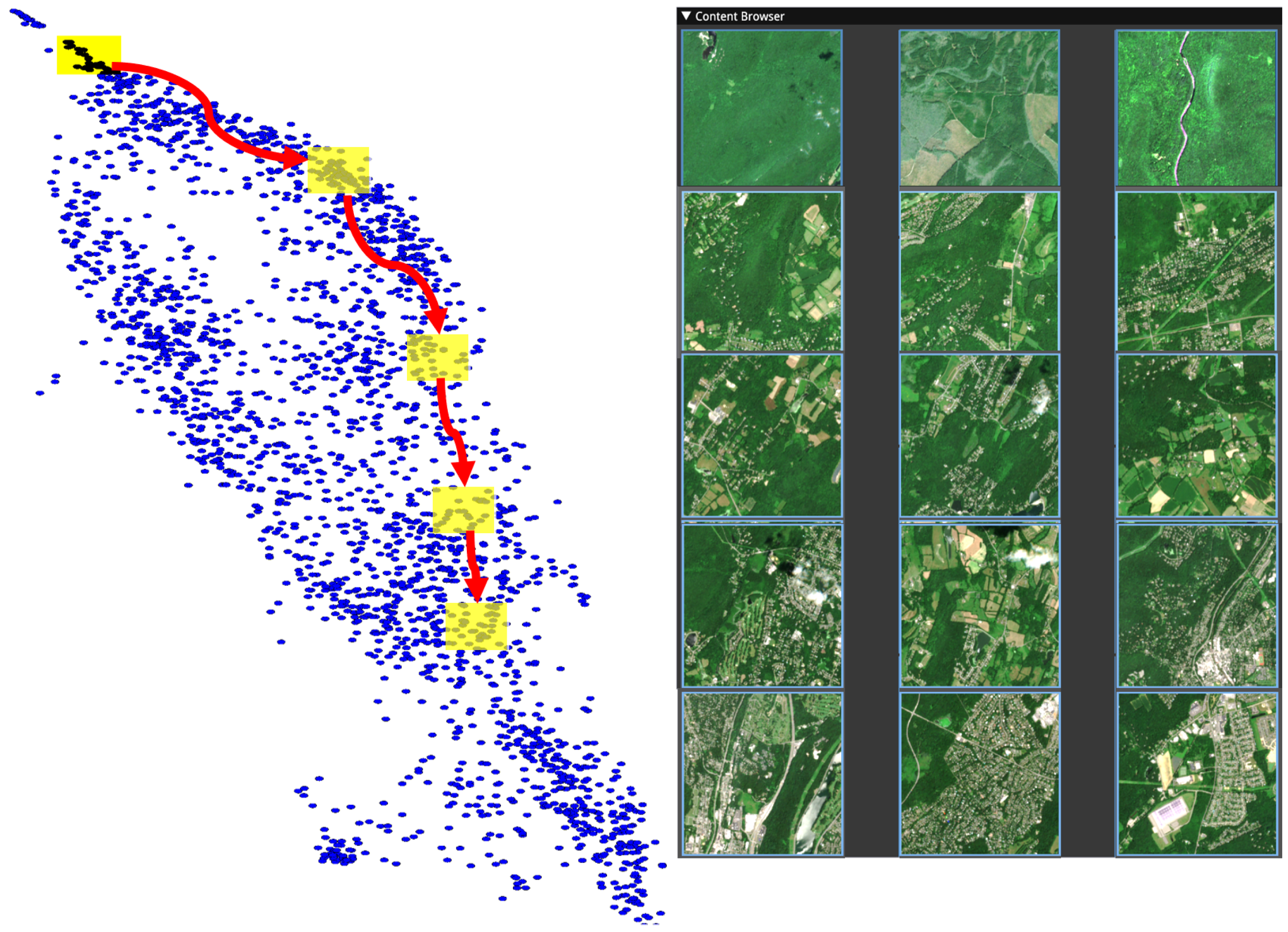
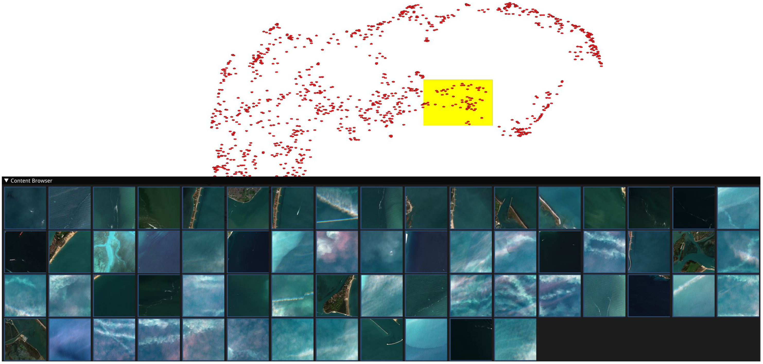
Manifold exploration: We explain how the user interacts with a two dimensional embedding to gain an understanding of the higher-dimensional manifold and to label multiple images simultaneously with a class label. The user draws a selection box of a desired size over the plot (yellow box in Figure 4). Each point within the selection corresponds to one image, which is displayed in the image browser and located on the map. All images within a selection can be given the same class label. If any images are not part of the class, they can be individually reset or set to a different class using the image browser. The user can navigate the scatter plot by scaling and translating.

The user drags the selection box so that points exit and neighbouring points enter the box. This simultaneously updates the image browser and map view, thus allowing the user to explore and become familiar with the structure of the manifold. Fine movement can help produce views where all images are consistent with one label, allowing a single label to be rapidly given to all points in the selection. In Figure 4, the user follows a path as indicated by the red arrows and yellow boxes, and sample images along the manifold from within the yellow boxes are presented in rows respective to the sampling region. These demonstrate how this model and two-dimensional embedding have placed images from the manifold. The block of images on the right shows three representative images from each of the indicated selection areas demonstrating the smooth evolution of the manifold from forest to urban land cover. 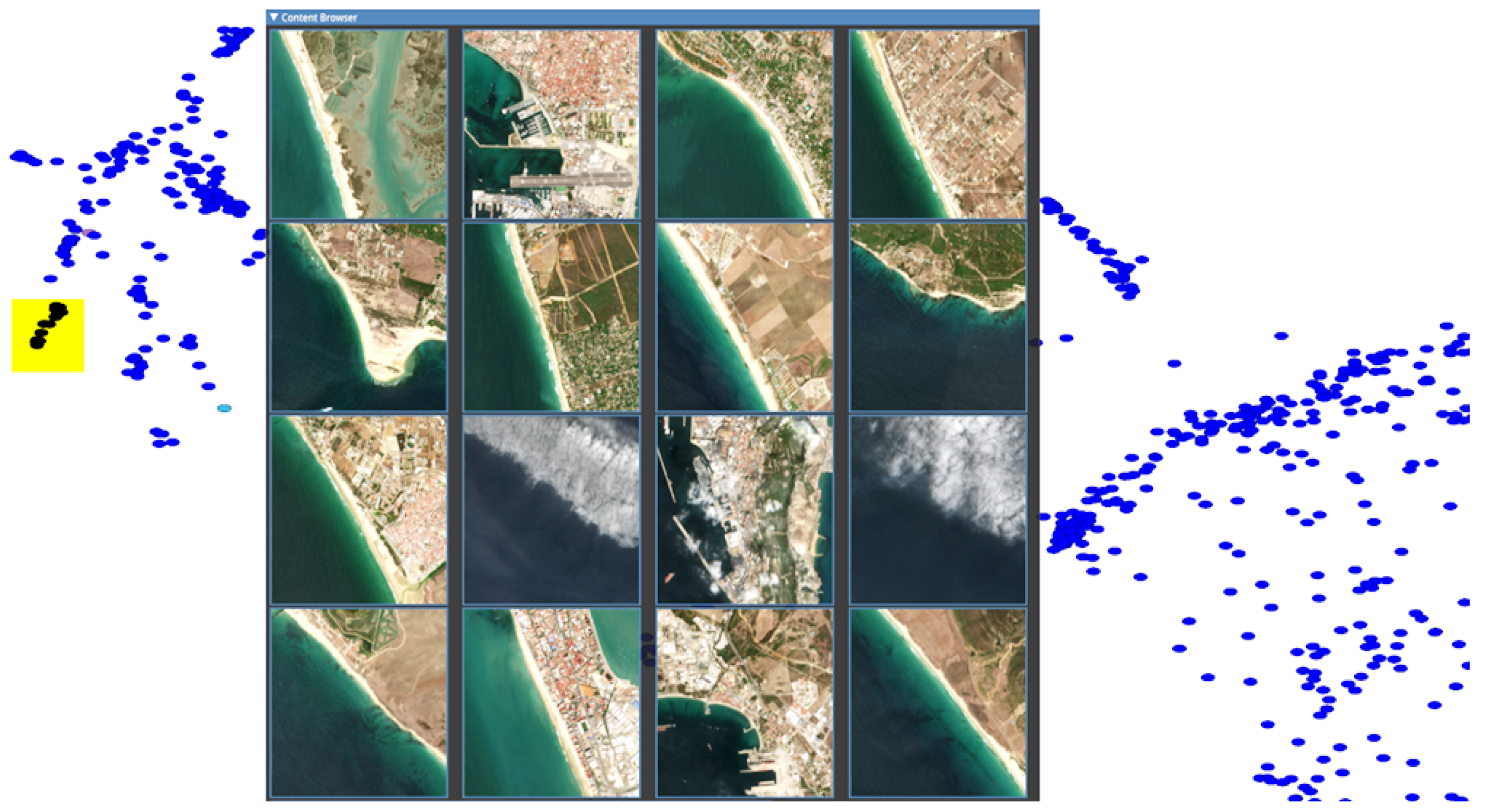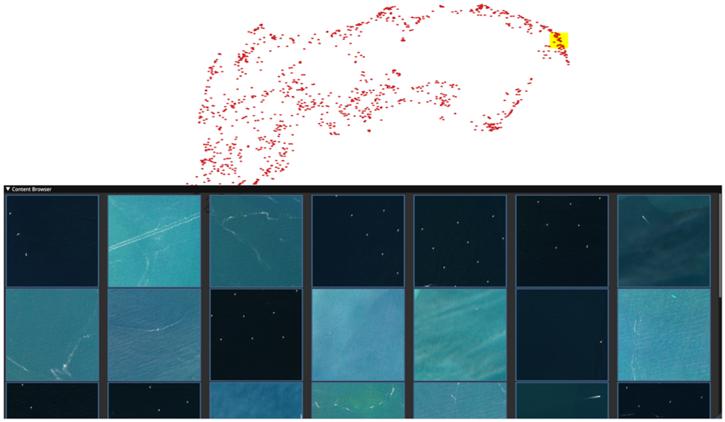Figure 5 shows 16 images in the browser window over the top of the scatterplot view. The images are from a small cluster on the left and show largely consistent clustering, but also demonstrate how the limits of a pre-trained model can affect labelling software. In this case, the reflectance and texture of cloud images have not been separated from the reflectance and texture of similar coastlines. The interface allows these labels to be quickly corrected individually. Users can label the data efficiently with a keyboard input as they explore the manifold.

Manifolds shown in the two-dimensional plot are formed by both the AE’s expressiveness on the source images and the number of samples that the DR technique is provided with. When projecting all images from the SWED dataset, there is a clear separation between land and water clusters, but images containing both features (coastline) are on the edges of those clusters or form paths between the clusters. See the video in additional material for an example of coastline labelling.

User-directed reprojection of the embedding: The two-dimensional scatter plot view may not be optimal due to two reasons. Firstly, the model’s latent space may not be expressive enough. Secondly, which is the focus of this section, the dimension reduction techniques have insufficiently exploited the latent space to successfully create the two-dimensional embedding. We work under the assumption that the AI model is fixed due to the fact that training remote sensing models requires a tremendous amount of resources, and therefore we cannot alter the latent space interactively. Rather, we look to optimise the embedding instead.

To find a better embedding we allow the user to direct re-embeddings by testing different parameters such as perplexity for t-SNE or N neighbours for UMAP. Increasing the value of both parameters allows for the DR algorithms to consider a larger neighbourhood, which provides more context to each embedded point. Conversely, if two manifolds exist in high dimensional space that overlaps frequently, a smaller neighbourhood of points would be preferable.

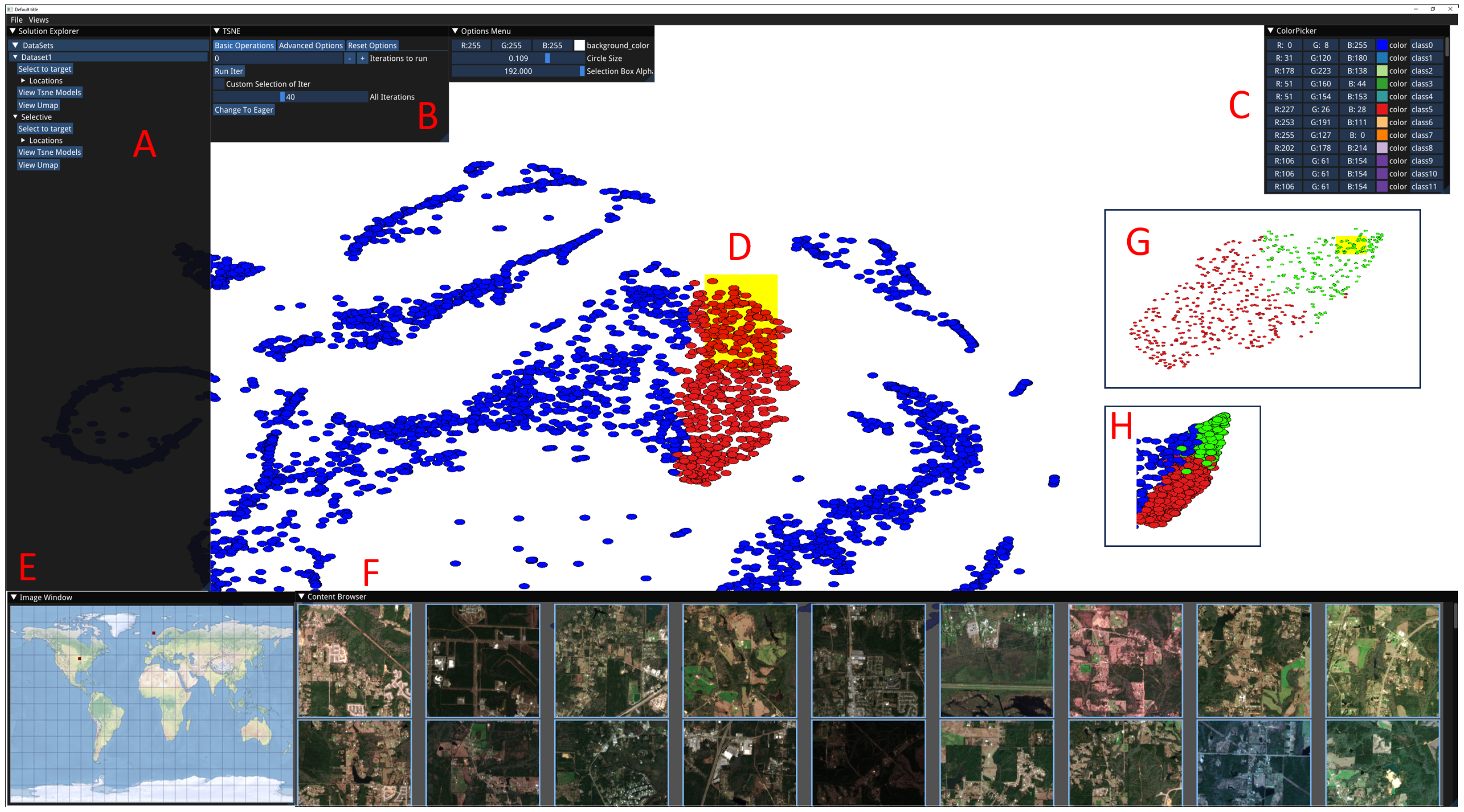
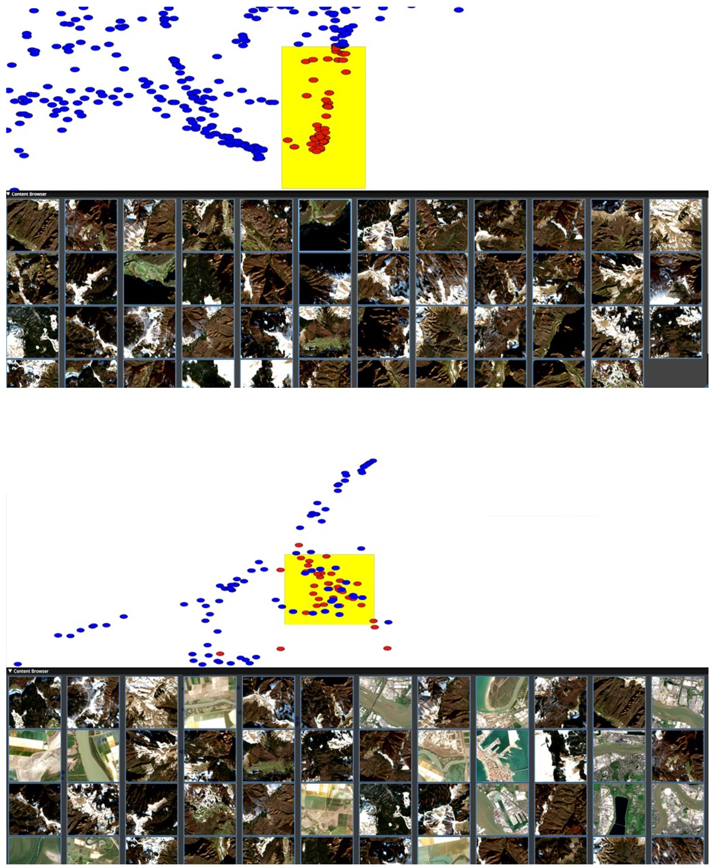
Therefore, it is crucial that the user can interact with parameter selection (B in Figure 3). However, recalculation of the embeddings on the entire dataset requires a high computational cost and exploration cost as new embeddings require validation of information patterns by the user. Constant evaluation of newly projected manifolds can be mitigated with our tool because labels can be extrapolated when switching embeddings (between UMAP and t-SNE) and when altering any of the parameters. This consistency in class labels can provide the user with context, e.g., how previously neighbouring points may now cluster or spread across the updated embeddings. In Figure 6, t-SNE (top) has clustered mountainous images (with glacier), allowing the user to apply a label with a single key press. Below, Figure 6, UMAP (bottom) has not differentiated such images from other terrain. By labelling using t-SNE, and then changing embeddings, we can see how the labelled points redistribute and mix within other samples. It is not generally the case that t-SNE performs better, rather being able to switch embeddings or re-embed using new parameters allows the user to find appropriate clusters.

Branch and merge: As an alternative to global embeddings, we introduced the ability to branch the dataset. Branching focuses the dimensionality reduction on the currently selected data. The two-dimensional embedding is optimised with respect to those samples as only those samples are considered. The computational cost is less due to the reduced number of samples when searching for optimal embedding parameters. The data for a particular branch is determined by the user indicating which class label or classes are to be used for that branch. All images labelled as that class form the branch. The user may select data directly on the two-dimensional plot using the selection box, apply a class label, and send that set of points to a branch. To self-contain branches, all embeddings utilise the UMAP or t-SNE algorithms for optimisation in their own sand-boxed environment without affecting any other dataset or branch.

Working with this reduced set of samples has two benefits. First, embeddings are faster to compute when varying parameters during exploration. Secondly, as the samples will have been determined by the user to have similarities, re-embedding them will effectively amplify the remaining feature differences yielding new clusters based on the alternate features. The new embedded clusters may separate better than the original given the same pre-trained model output.

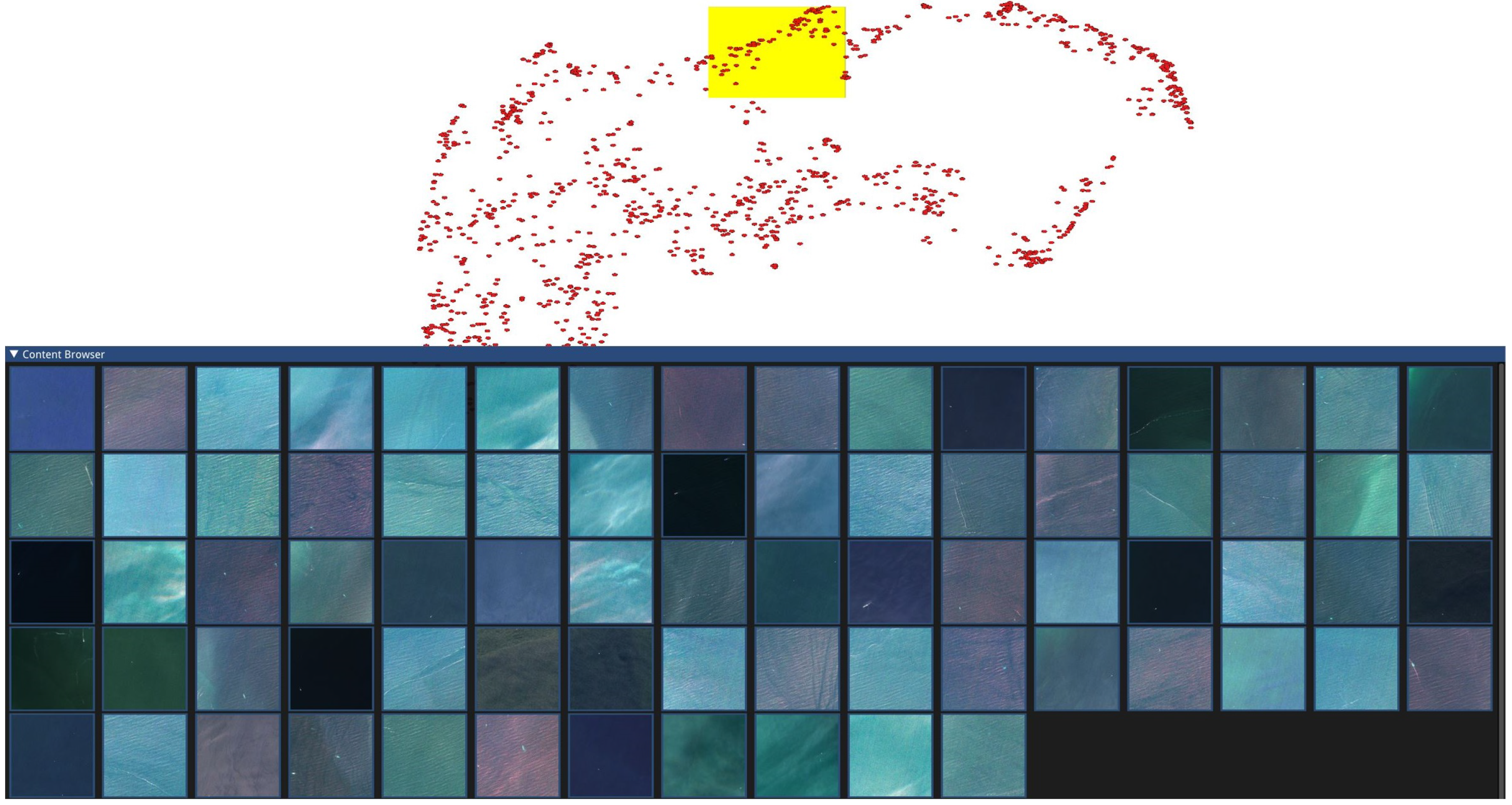
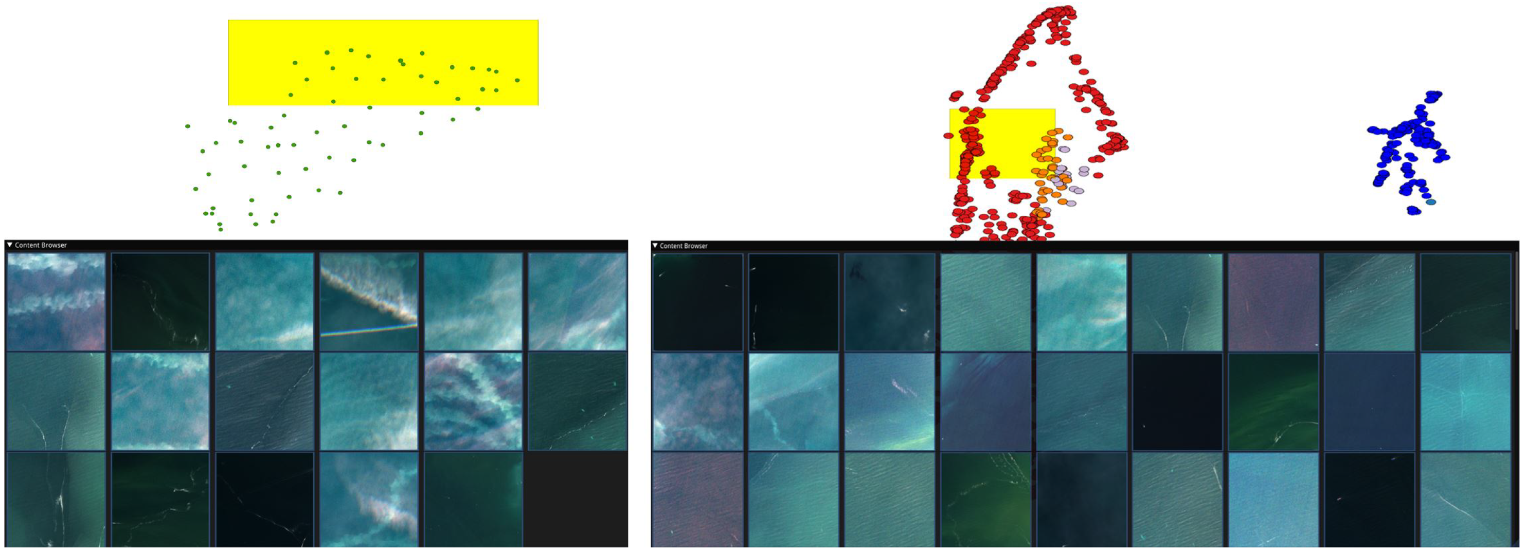
Figure 7 shows a branch of data from Figure 5, which largely represents images with only sea and varying coverage of coastline. In the global embedding, they clump together in a smaller cluster in which it would be difficult to make selections that separate these classes for labelling. Branching out these points allows a re-embedded of the points, resulting in the embedding seen in Figure 7. In this case, the points scattered along the top of the new plot are predominantly the images that contain just the sea, allowing the user to make large selections of tens to hundreds of images and directly apply one class label.

Moving along the top of the plot and to the right (Figure 8) introduces a new wind farm feature where we can see a regular grid of white turbines against the dark blue sea suggesting the user would be able to quickly label sea infrastructure as a separate class if desired.

Further around the plot (Figure 9) there is a mix of coast, high cloud and sea that has not been effectively separated and therefore would be time-consuming to label. This can also be branched out into its own where the sea is more effectively separated in this new embedding (Figure 10 (left)). Labels are then merged back into the main embedding (Figure 10 (right)) showing the separation (or lack of) between these classes. This allows fast labelling of the data, which also allows the user to visualise the class boundary, allowing an assessment of model performance by suggesting where the model may be failing to provide good class separation.

We also find that branching is effective in another way. If a user wants to label patches with multiple features, for example, coastal areas with farmland present, they can branch and embed all coastal patches together with a selection of patches that contain only farmland. The embedding will create unique clusters for each feature; however, samples that have both features will lie on the edge of the cluster closest to the cluster that contains the other feature. In this case, samples with both coastline and farmland will be on the edge of the coastline cluster closest to the cluster containing purely farmland. In this way, branching can act as a way to query image features in clusters by leveraging the model’s general ability to distinguish between them.

User Study

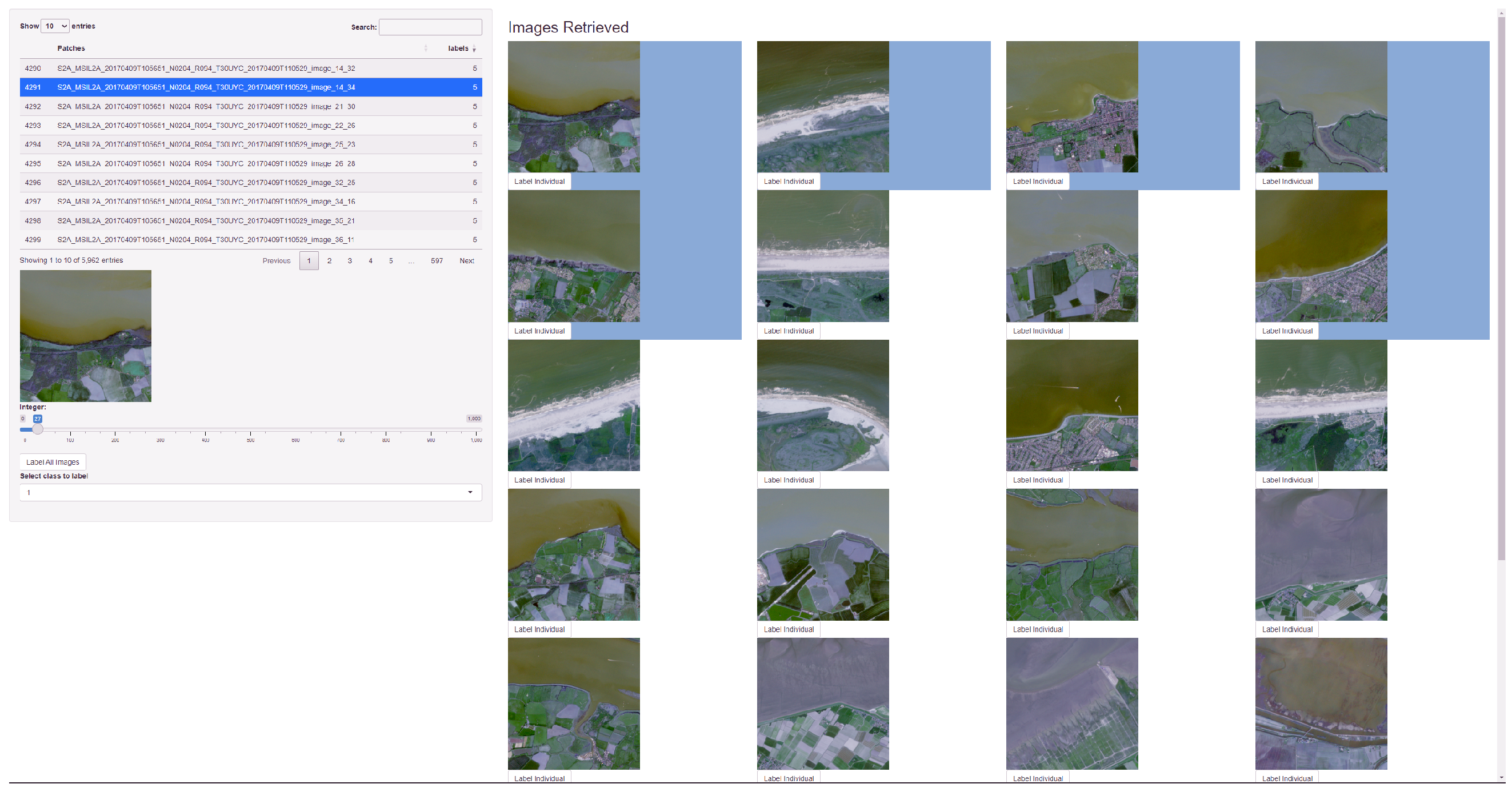
In this section, we introduce a second application (Figure 11) to act as a comparison in a user study. We compare the efficiency of finding coastal patches utilising an image retrieval application as a benchmark, as our pipeline can be interpreted as a visual extension of image retrieval systems. The benchmark application produces K similar images based on a query image. The K nearest neighbours are determined by distance in the autoencoder latent space. The target query image is shown with the most similar K images. The user can label all images returned by the query or individually label each sample.

To access the capability of each application we conducted a small user study with five participants. The user study consisted of each applicant labelling patches with any coastline utilising both applications. We presented the participants with forty initial “seed” images, as otherwise, the benchmark application required sorting through a list of 5963 patches to find an initial coastal patch to begin labelling from. The same “seed” patches are pre-labelled within our application as one class.

The task was to label 160 patches with coastline using each application. We allowed participants to label more patches than required accounting for any scenarios where labels were assigned with the intention to refine after. The method to end the study was based on a small GUI element that let the researcher know that the labelling requirement had been met, allowing them to make an informed decision on when to let the participant stop labelling. We switched the order in which both applications were presented to each user in order to keep any familiarity gained with RS images consistent. As both t-SNE and Umap are stochastic algorithms we retained the initial randomisation seed between participants. In addition, we removed multi-threading and approximations utilised by the dimensionality reduction algorithms in order to keep consistency between participants. Times were recorded for each patch labelled. In order to produce the results, any patches labelled multiple times were removed with only the final label assignment considered.

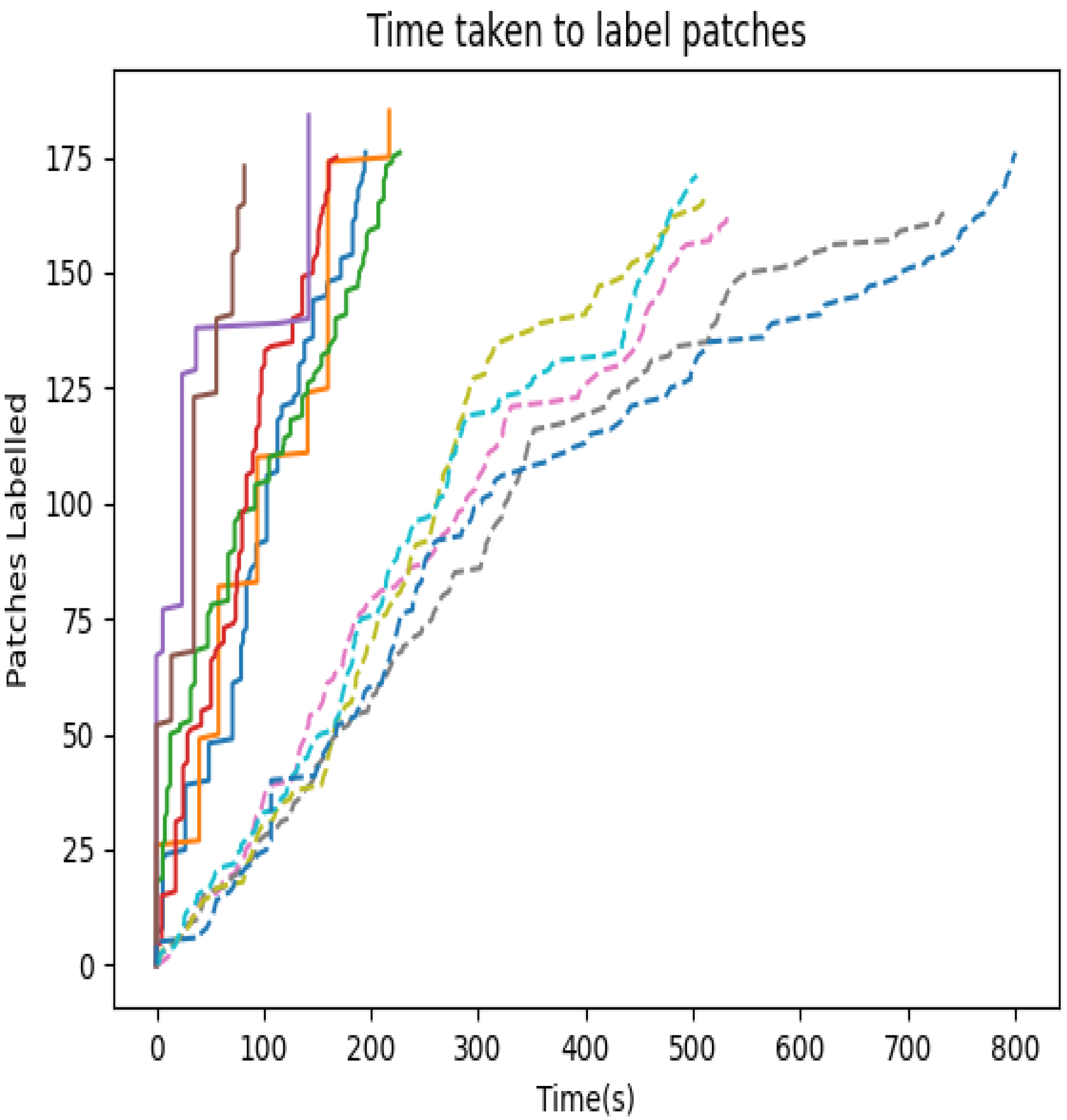
The results of the user study are shown in Figure 12. On average, the time taken to label using the benchmark application was 269 s compared to our application’s 71 s, which is a factor of more than 3 times faster. Users utilising the benchmark application often found that only a small number of patches could be retrieved without the appearance of out-of-class images, which reduced the ability to label all samples quickly and efficiently therefore resulting in single sample labelling. In contrast, in our approach, the ability to optimise the box size and explore its surroundings produced similar images within the embedding, allowing the user to discern a suitable selection, which retained minimal out-of-sample patches and allowed the user to refine the selection with more confidence. The fastest user strategy recorded utilising our application searched the space before selecting clusters with more coherent samples and only a few outliers. In contrast, the other common labelling strategy used was panning a small selection area with continuous movement and refinement. The difference can be seen in Figure 12. The sharp increase in labels corresponds to labels applied to a larger selection area at once in contrast to the smoother gradient when labelling with a small selection strategy, respectively. It is also noticeable that users of the benchmark application experienced fatigue as they approached the target and had difficulties finding more coastline to label, whereas users of our application did not experience that problem. This is visible in the shallower gradients in the data for the benchmark application as time goes on compared to the steeper gradient for our application.

4. Discussion

Designing a training and testing dataset for the development of computer vision algorithms for use in satellite imagery is time-consuming, resource-intensive and uncertain. It is difficult to be confident that a labelled dataset encompasses sufficient complexity and diversity to allow for the geographic generalisation of a trained algorithm to unseen areas. It is practically difficult to visualise large and geographically distributed datasets and “debug” the performance of a trained algorithm once its performance is assessed against a test dataset.

Our tool offers new capabilities for us to reduce the time and resources required to label large datasets, visualise and understand the complexity and diversity of already labelled images, and assess model performance against clusters of similar image types, which might be geographically distributed over large and diverse environments. Overall, our tool will give us greater insight into the structure of unstructured satellite imagery data, supporting us to iterate model development with greater efficiency and confidence.

With regard to processing and labelling datasets for future training of classification models, we have shown how structurally similar samples are clustered together and evolve along a manifold, allowing for the intuitive selection of samples from all geographical regions. Samples evolve as you move from a cluster, where samples with more unique features appear on the cluster boundaries. Users are able to select and label similar features and build up feature-rich data sets.

Most works in remote sensing target specific regional locations to alleviate the vast complexity between tile locations and time. Utilising our tool, we show how analysis of multiple tile locations beforehand could contribute to providing balanced datasets for future classification tasks. User-led mass labelling could provide more contextual information based on the classification goal, e.g., lakes, farmland use, arboreal or coastline to name a few.

Common image dataset tools in current works regard finding the top K images that correspond to a query set of images. Most, such as Tong et al. [40], produce feature sets using common image retrieval algorithms and fine-tuning with smaller patch sizes, but based on higher resolution labelled datasets. We have in comparison shown the feasibility of utilising manifold learning techniques to enable entire datasets and relationships between images to be displayed. This has been effective in mass labelling larger feature sets. When considering smaller local features, we utilise our branching methodology. Future work could also encode smaller patches with extra information regarding surrounding patches, increasing the focus on smaller features, but retaining a more global context. This of course would have to be balanced between computational efficiency for embeddings as larger latent spaces or sample rates increase the time complexity to calculate embeddings.

In comparison, for better potential label separation, we could iteratively alter our higher dimensional space by pushing dissimilar images from an oracle or user’s perspective away and pulling similar images closer. This process in machine learning is known as triplet loss [41]. Successfully applying triplet loss improves the downstream visualisation capabilities as manifolds separate clearly. However, this process would require retraining on the new high-dimensional embedding space, and constant oracle/human input where labels can heavily influence models’ class separation. With such feature-rich patches, this could cause overlap between labelling categorisation, for example, where a particular patch includes multiple regions of interest, i.e., farmland and rivers. An avenue for future work could look to implement a form of triplet loss with a multi-hierarchical labelling scheme utilising the visual branching feature we presented.

In addition, the utility of understanding the performance of a model between the RS images utilised in training and the resulting complex learnt filters by the convolutional AE is paramount in any use case. The user can gain estimations of model performance by altering the manifold learning representations and examining the visualisation provided by the projected manifold. Our methodology could be adapted to any model where a temporary layer can be trained to extract an embedding space. Limitations are the size of the representation of each image, larger high-dimensional spaces require more time to project. The resulting embeddings within the tool provide contextual information about how samples are built by the model and where problematic features may arise in images.