A Decision-Making Model to Determine Dynamic Facility Locations for a Disaster Logistic Planning Problem Using Deep Learning

Abstract

Disaster logistics management is vital in planning and organizing humanitarian assistance distribution. The planning problem faces challenges, such as coordinating the allocation and distribution of essential resources while considering the severity of the disaster, population density, and accessibility. This study proposes an optimized disaster relief management model, including distribution center placement, demand point prediction, prohibited route mapping, and efficient relief goods distribution. A dynamic model predicts the location of post-disaster distribution centers using the K-Means method based on impacted demand points’ positions. Artificial Neural Networks (ANN) aid in predicting assistance requests around formed distribution centers. The forbidden route model maps permitted and prohibited routes while considering constraints to enhance relief supply distribution efficacy. The objective function aims to minimize both cost and time in post-disaster aid distribution. The model deep location routing problem (DLRP) effectively handles mixed nonlinear multi-objective programming, choosing the best forbidden routes. The combination of these models provides a comprehensive framework for optimizing disaster relief management, resulting in more effective and responsive disaster handling. Numerical examples show the model’s effectiveness in solving complex humanitarian logistics problems with lower computation time, which is crucial for quick decision making during disasters.

1. Introduction

Disaster logistics management, which involves planning and organizing the distribution of logistics to provide humanitarian assistance, is an important aspect of disaster management. It is crucial to minimize human suffering, property loss, and ensure a timely and appropriate response.

However, disaster logistics management frequently faces a number of challenges. First, disaster relief logistics costs can reach up to 80% of total aid costs [1,2], making logistics one of the most expensive components of disaster management [3]. Second, logistics management occurs frequently because aid distribution is not on target or evenly distributed [4]. This is due to the selection of unsuitable distribution center locations and distribution routes that have not reached the expected level of effectiveness.

A dynamic facility location problem model for managing humanitarian aid logistics is required to overcome problems in the management of humanitarian aid in post-disaster areas. The problem of locating emergency facilities is the most fundamental humanitarian logistical problem. The problem of locating emergency facilities following a disaster is related to the location routing problem (LRP), which is used to optimize the location allocation of facilities and routes for humanitarian aid delivery. LRP problems are difficult combinatorial problems that are frequently categorized as NP-hard [5,6]. LRP combines two kinds of problems: facility location problems and vehicle routing problems. The combination of these two issues makes LRP a difficult problem because it necessitates complex decision making when selecting the location of facilities and efficiently planning vehicle routes.

Several models and approaches have been proposed to address the location facility problem in relief logistics and LRP management, including MOGWO, MOPSO, MOWCA, NSGA-II [7], hybrid genetics (genetics and NSGA-II) [8], a combination of the multi-objective simulated annealing algorithm (MOSA) and non-dominated sorting genetic algorithm II (NSGA II) [9], a combination of discrete particle swarm optimization (DPSO) and Harris Hawks optimization (HHO) [10], greedy algorithm [11,12], tabu search [10,13,14,15], mixed integer linear programming (MILP) [16], mixed integer non-linear programming (MINLP) [17], particle swarm optimization (PSO) [18], and e-constraints [19,20,21,22]. Based on the research described, it is possible to conclude that the LRP can be solved using two approaches: the exact approach and the heuristic approach. Because the exact method takes a solution-finding approach by calculating every possible solution to produce the optimal answer, the exact algorithm takes a long time to complete to produce an optimal answer for large-scale problems. In the case of optimization problems, heuristics is a rule-of-thumb approach that allows for solutions that are not convergent or optimal [23]. As a result, the goal of this research is to create a model for dealing with LRP in the context of disaster relief logistics. Several researchers propose an artificial intelligence approach to optimize the objective function and address the solution problem in LRP [24].

Deep learning is a machine learning method that employs deep and complex artificial neural networks to extract patterns and features from data [25]. Several studies using the deep learning approach have made significant contributions to disaster management problem solving [26]. Methods such as convolutional neural networks (CNNs) [27,28,29], combined convolutional neural networks (CNNs) and support vector machines (SVMs) [30], combined deep belief networks (DBNs) and restricted Boltzmann machines (RBMs) [31], long short-term memory (LSTM) neural networks [32,33], artificial neural networks (ANNs) [34], neural network algorithms based on rough set and radial basis function (RBF) [35], and recurrent neural networks (RNNs) [36,37] are used to predict disaster risk, identify affected areas, map landslide and flood vulnerabilities, and recognize post-disaster building damage. Meanwhile, most current research on disaster logistics employs exact or heuristic approaches in determining the location of emergency facilities and routes for sending aid. In this context, there is an unmet need to solve location facility problems for disaster logistics using a deep learning approach. Deep learning can provide innovation and excellence in handling LRP in a more efficient and accurate manner. The development and application of deep learning in the context of disaster logistics management therefore presents significant research opportunities.

Therefore, this study aims to fill this research gap by developing a deep location routing problem (DLRP) model, which is dynamic and capable of recommending the opening of distribution centers (DC) based on demand point locations using the K-means method. It also utilizes deep learning to predict the locations of demand points at formed DCs in the context of disaster management, and the formation of disaster relief delivery routes using artificial neural networks (ANN). Additionally, a forbidden route model is established to select the existing routes and map them as either prohibited or permissible routes, resulting in a bi-objective mixed-integer nonlinear programming model with two objectives: minimizing cost and minimizing time. Thus, by incorporating a deep learning approach into solving location facility problems for disaster logistics, this research can significantly contribute to the field.

The remainder of this paper is organized as follows. Section 2 begins with a description of the problem, model assumptions, the model objective function, formulating model constraints, and modeling by developing a location routing problem (LRP) model with a deep learning approach called the deep location routing problem (DLRP). This includes a dynamic emergency facility location model, prediction model, transportation route formation, and optimal route, which includes forbidden routes to generate an optimal route with the objective function of minimizing cost and time. Section 3 includes numerical studies to demonstrate the properties of the proposed model and algorithm. Finally, Section 4 concludes this paper.

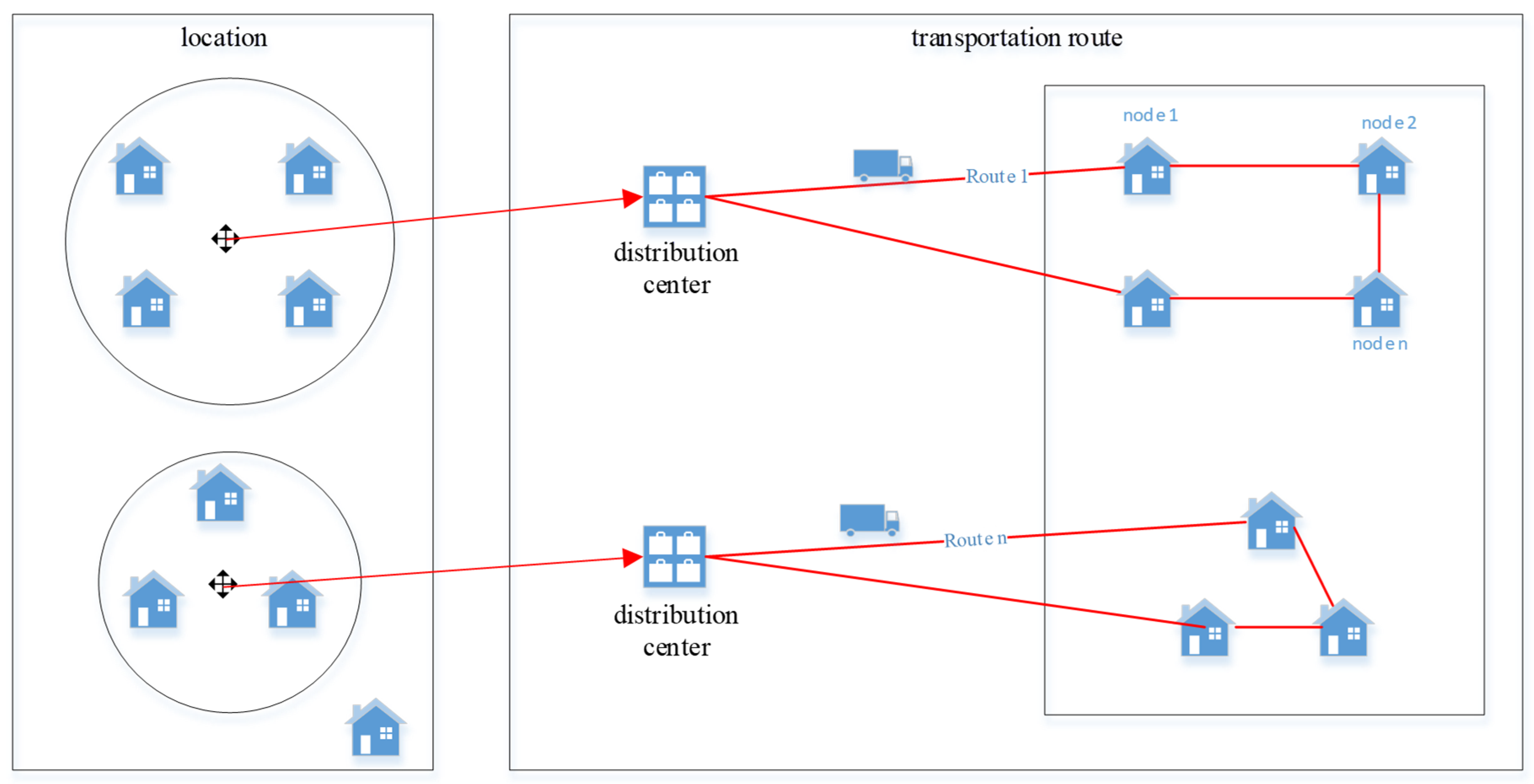
2. Problem Description

The following is a description of the problem in the formation of distribution routes in humanitarian logistics, including the distribution center, demand point, and vehicle parameters.

Figure 1 depicts an illustration of the problem, which describes the planning of transportation routes with uncertain parameters; namely, demand points and vehicles. We obtained a description of the problem based on these parameters, which includes: first, determining the distribution center development point after a disaster that has the shortest distance to the point of demand; second, if given a set of vehicles, how are these vehicles assigned to each open distribution center; and third, forming transportation routes from clusters formed based on assigned vehicles.

2.1. Model Assumptions

The model’s assumptions for establishing transportation routes in post-disaster areas under uncertainty are as follows:

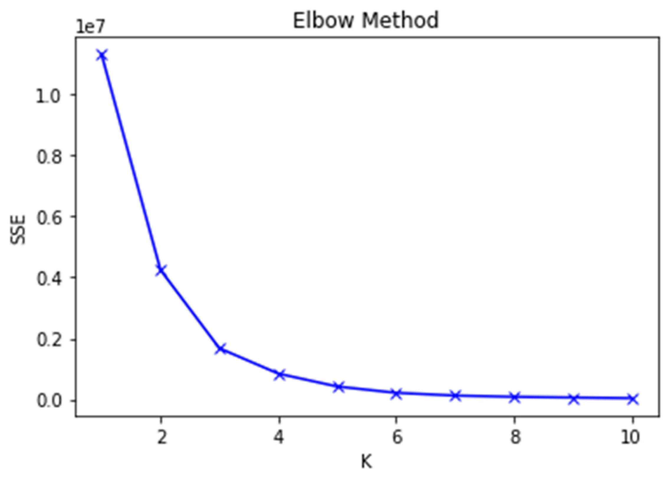
• determining the number of distribution centers that will be opened in the aftermath of a disaster;
• grouping demand points based on the shortest distance between opened distribution centers;
• forecast the location of newly opened distribution centers;
• determine which vehicles are assigned to newly opened distribution centers;
• determine clusters based on vehicle capacity and number of vehicles—the network only includes demand points that can be visited via the traffic network, and ignores areas that require other special modes of transportation;
• Each vehicle has a limited capacity—each vehicle begins and ends at the distribution center to which it belongs while completing the delivery task to the point of demand, and each point of demand is only visited once, where the route of distribution of relief goods is uncertain.

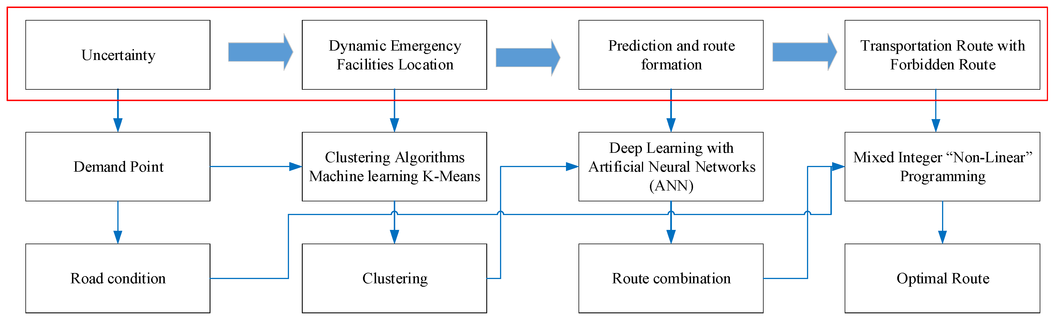
2.2. Objective Function

The transportation route formation model’s objective function in post-disaster areas with uncertainty in humanitarian logistics is:

1.

Location of emergency facilities

• The emergency facility location model generates an objective function based on the shortest distance between open distribution centers and demand points ($min{\sum }_{ij}distance$).

2.

Predicting location and forming transportation routes

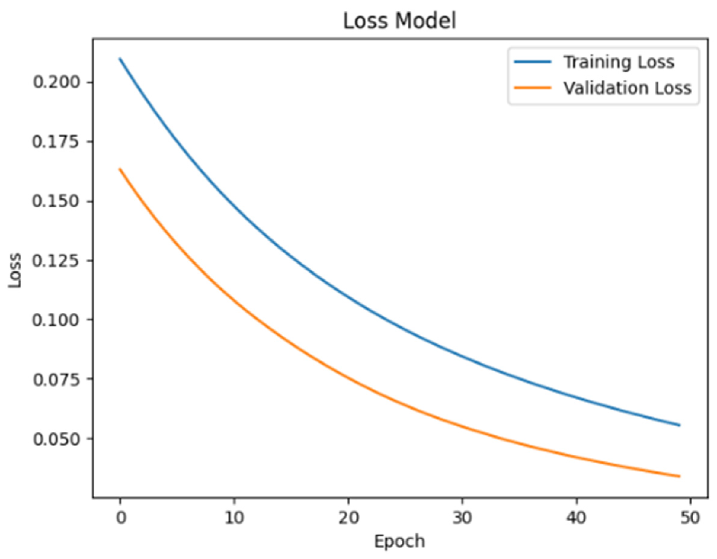
• Based on open distribution centers, the location prediction model forecasts locations. The model is then trained by displaying an increase in accuracy, indicating that the model is still optimizing its internal parameter adjustments to improve performance, which has the potential to provide reliable predictive results and can be used effectively in relevant contexts such as predicting locations or data classification. The formation of transportation routes yields a destination function, which is a combination of routes based on demand point clusters $\left(\bigcup _{i=1}^{i=n}L\right)$.

3.

Distribution route in uncertainty

• The forbidden route model, which is used to optimize route planning in routing problems with forbidden route restrictions, is used for distribution routes that are subject to uncertainty. Every vehicle used in this model will not take the forbidden route. The model’s objective function is to minimize the total cost ($h)$ and arrival time ($w)$ of the vehicle at the demand point $\left(\genfrac{}{}{0pt}{}{\mathrm{Min}}{x,y,z,q}{\mathcal{z}}_1\left(D\right)=\left\{w,h\right\}\right)$ of a route that is not prohibited.

2.3. Formulate Model Constraints

Model constraints for the formation of transportation routes—first, the model constrains for opening the location of emergency facilities and the demand point clusters, including determining the distribution center point based on the closest distance to the demand point or the demand point cluster based on the nearest distribution center. Second, the model constrains for route formation, including the number of routes for each cluster based on the capacity and the number of vehicles assigned to the distribution center, the combination of routes based on demand points in the cluster, and the route selection based on conditions in which each demand point is only visited once.

2.4. Modelling

The schematic diagram of the model for forming transportation routes in humanitarian logistics using a deep learning approach can be seen in Figure 2.

Based on Figure 2, there are uncertainty parameters, including demand points used for opening emergency facility locations, namely distribution centers. In this case, machine learning clustering algorithms, namely K-Means, will be grouped based on similar demand points, such as the coordinate points (latitude, longitude) depicted in Figure 3.

After obtaining the grouping results in Figure 3, the location for opening a dynamic distribution center—one that can move based on the number and location of demand point locations—will be determined. In order to achieve the minimum distance objective function, the distribution’s opening will be taken from the centroid location based on the cluster that has been formed. Figure 4 depicts how to determine the location of emergency facilities and group demand points based on assigned distribution centers. Following the acquisition of distribution center locations and the grouping of demand points, a route formation process will be carried out, which will employ a deep learning approach with deep neural network architecture. The combination of routes will be determined based on the distribution center, number of vehicles, number of demand points, and number of demands. Figure 4 illustrates the formation of a route using deep learning models built on an artificial neural network (ANN) architecture.

Before establishing a route, the first step in Figure 4 is clustering using a machine learning algorithm to determine the location point for opening a distribution center, and grouping demand points based on distribution centers and assigned vehicles. The location of a distribution center is determined dynamically based on the location of the demand point following the disaster. The results of opening emergency facility locations are used as input $\left(x\right)$ for route formation.

Deep learning neural network algorithms, also known as artificial neural networks (ANN), are used to create a network of routes for the distribution of relief goods from the distribution center to the point of demand. The input layer consists of distribution center location data and demand points in one cluster, the hidden layer represents the spread of the location of the request points, and the output layer shows the result of a combination of location distributions resulting in the formation of routes.

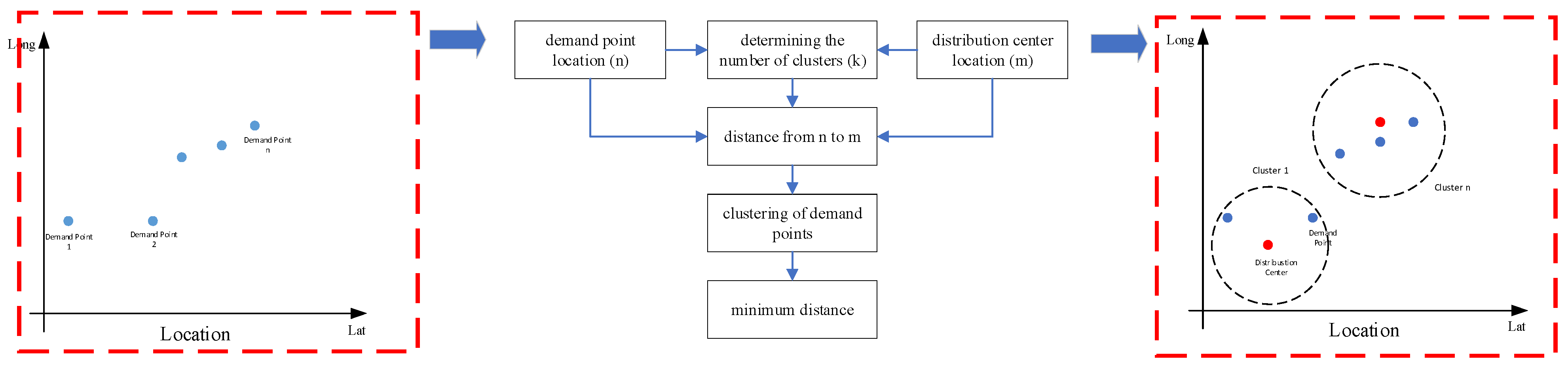
2.4.1. Emergency Facility Location Model

The k-means clustering machine learning algorithm is utilized as the basis for determining the location of distribution centers and grouping demand points. The algorithm divides a set of N objects into K clusters based on the similarity between members within each cluster and dissimilarity with members in other clusters [38]. The similarity to the cluster is measured by the proximity of each object to the cluster’s mean value, known as the cluster centroid.

The core concept of the K-means algorithm involves iteratively searching for cluster centers. The cluster center is determined based on the distance between each data point and the cluster center. The clustering process begins by identifying the data to be clustered, denoted as $x_{ij} \left(i=1,\dots ,n;j=1,\dots ,m\right)$, where $n$ represents the total number of data points to be clustered and $m$ represents the number of variables. At the start of the iteration, each cluster’s center, $c_{kj} \left(k=1,\dots ,K;j=1,\dots ,m\right)$, is assigned independently and arbitrarily.

Next, the distance between each data point and each cluster center is computed. The Euclidean formula is commonly used to calculate the distance $d_{ik}$ between the $i^{\mathrm{th}}$ data point $\left(X_i\right)$ and the $k$^th cluster center $\left(C_k\right)$. If the distance between a data point and the center of the $J$-cluster is smaller than the distance to the centers of other clusters, the data point is assigned as a member of the $J$-cluster.

After assigning data points to their respective clusters, the next step is to group the data that belong to each cluster. The new cluster center value can be calculated by determining the average value of the data points that are members of the cluster.

• Notation:

• $m$: number of distribution centers (DC) with $i=1,\dots ,n$
• $n$: total of demand points with $j=1,\dots ,n$
• $c$: latitude and longitude coordinates
• $K_{jc}$: $c$ is the coordinates (lat, long) of the demand point $j$
• Variables:
• $f_{ic}$: coordinates $k$ of DC $i$
• $D_{ij}$: distance between DC $i$ and demand point $j$
• $X_{ij}$: 1 if demand point $j$ is assigned to DC cluster $i$, and 0 otherwise
• Formulation

When the location of the demand point $\left(n\right)$ is known, the determination of the distribution center’s location $\left(m\right)$ is formulated with a single objective.

$$\min {\sum }_{ij}{D}_{ij}{y}_{ij}$$

(1)

Subject to:

$${\sum }_j{y}_{ij}=1,{\forall }_i$$

(2)

$$D_{ij}=\mathrm{euclidean} \mathrm{distance}\left(f_i,d_j\right),{\forall }_{i,j}$$

(3)

$$y_{ij}\in \left(\mathrm{0,1}\right)$$

(4)

Equation (1) minimizes the distance between distribution center $i$ and the collection of demand points $j$, while Constraint (2) ensures that all demand points $j$ are in the same cluster as distribution center $i$. Constraint (3) defines the distances between distribution center $i$ and demand point $j$, while Constraint (4) represents binary decision variables.

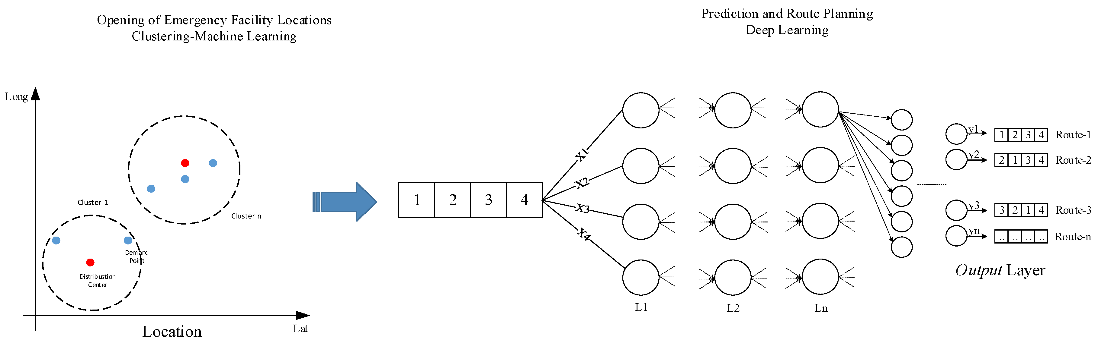
2.4.2. Model Prediction and Transportation Route Formation

• Predictions

In the prediction model described below, $X$ represents the input data, while y represents the target label or class. The model, generated using the provided code, consists of two hidden layers, each containing 64 neurons. The output layer consists of three neurons, applying the ReLU (Rectified Linear Unit) activation function to the hidden layers, and softmax activation function to the output layer. The optimizer used in training the model is Adam, and the loss function employed is sparse categorical cross-entropy, as demonstrated below.

• # Step 1: Load data from a CSV file (‘data.csv’):
• data = load_csv(‘data.csv’)
• # Step 2: Separate attributes (attribute1, attribute2, …) and labels (label) from the data:
• attributes = data[[‘attribute1’, ‘attribute2’, …]]
• labels = data[‘label’]
• # Step 3: Split the data into training data (X_train, y_train) and test data (X_test, y_test) with a test size of 20%:
• (X_train, X_test, y_train, y_test) = split_data(attributes, labels, test_size = 0.2)
• # Step 4: Normalize training and test data using StandardScaler:
• X_train = normalize(X_train)
• X_test = normalize(X_test)
• # Step 5: Initialize an artificial neural network (ANN) model:
• model = initialize_model()
• # Step 6: Compile the model:
• compile_model(model)
• # Step 7: Train the model with training data:
• train_model(model, X_train, y_train, epochs = n_epochs, batch_size = batch_size)
• # Step 8: Evaluate the model on test data:
• (loss, accuracy) = evaluate_model(model, X_test, y_test)
• print(‘Loss: {:.2f}, Accuracy: {:.2f}%’.format(loss, accuracy * 100))
• # Step 9: Transform new data for prediction after normalization:
• new_data = normalize_new_data([[new_attr1, new_attr2, …]])
• # Step 10: Make predictions using the trained model:
• predictions = make_predictions(model, new_data)
• # Step 11: Initialize the same model for grid search:
• grid_search_model = initialize_model()
• # Step 12: Compile the grid search model:
• compile_model(grid_search_model)
• # Step 13: Perform grid search to find optimal model parameters with training data:
• best_model = perform_grid_search(X_train, y_train, grid_search_model, param_grid, cv = 3)
• # Step 14: Use the best model to make predictions on new data:
• new_predictions = make_predictions(best_model, new_data)

b.

Route Formation

The formation of transportation routes in humanitarian logistics utilizes deep learning neural network algorithms, specifically artificial neural networks (ANN). Figure 3 illustrates the ANN structure employed in the creation of these routes.

The input layer of the ANN is derived from the grouping of demand points J based on the assigned DC $i$ and vehicle $k$. The hidden layer in the ANN represents the transformation of information from the location of the demand point $j$. The output layer then combines this location distribution by incorporating the location of the demand point $j$ from the hidden layer $L_{ij}$. As a result of this combination, the $Y_i$ route is formed.

Upon combining the routes, a route selection process is conducted to ensure that each demand point is visited only once. This selection process helps optimize the transportation routes. The vehicles follow the selected routes, starting from DC $i$ and returning to the same DC $i$, which is assigned to a specific cluster $k$. By limiting the visits to each demand point and establishing a circular route from and back to the distribution center, the transportation process becomes more efficient and organized within the designated cluster.

• Variables:
• $y_i$: Route $i$
• $L_{i,j}$: Demand point location
• Formulation

Once the grouping is generated, the formation of N transportation routes is formulated using a deep learning model known as an artificial neural network (ANN).

$$y_i=\bigcup _{i=1}^{i=n}{L}_{i,j}$$

(5)

where,

$$y_i=\left\{\begin{array}{c}1, L_{ij}\ne L_{ij}\\ 0,L_{ij}=L_{ij}\end{array}\right.$$

(6)

Equation (5) is utilized to form the transportation route based on the distribution of demand point locations $\left(L_n\right)$. This equation captures the process of determining the optimal route considering the specific distribution center and cluster assignment.

Furthermore, Equation (6) incorporates the route selection mechanism, which ensures that each demand point is visited only once. By imposing this constraint, the transportation route is designed to efficiently cover all the required demand points without revisiting any of them.

The vehicles follow the established transportation route, commencing from the assigned DC $i$ distribution center IK and returning to the same DC $i$ within the designated cluster $k$. This approach helps streamline the logistics process and ensure effective distribution of goods.

2.4.3. Optimal Route

In the given context, a set $X$ is provided which contains prohibited routes. A route $\left(v_1,\dots ,v_l,\right)$ is considered avoided from set $A$ if none of its subroutes $\left(v_i,\dots ,v_j,\right)$ are included in set $A$, for any pair $i$ and $j$ where $1\le i<j\le l$.

When discussing the shortest route that avoids set $A$, a route $P$ from $s$ to $t$ is considered the shortest if the distance traveled along route $P$ is the shortest among all routes that avoid set $A$ when traveling from $s$ to $t$.

In the specific case where set $A$ is equal to set $X$, which represents all the forbidden routes in the graph, the term “exception avoiding” is used instead of “$X$-avoiding” in this context. It is also crucial to ensure that the request point does not fall on any prohibited route. Each vehicle used in this model will strictly avoid traveling through any of the forbidden routes, adhering to the imposed restrictions and constraints.

• Notation:
• $R$: Set of resources used
• $C$: Set of customers
• $X$: Set of forbidden route
• Variables:
• ${\overline{\mathcal{z}}}_1\left(D\right)$: Cost and time of arc $(i,j)$
• $x_{ij}$: Binary variable indicating whether arc $(i,j)$ is used in the route or not
• $d^{+}\left(i\right)$: The set of arcs comes out of vertex $i$
• $d^{-}\left(i\right)$: The set of arcs enters node $i$
• $T_{ij}^r$: The time required to travel from node $j$ to node $i$ uses resource $r$
• $a_i^r$ and $b_i^r$: The initial time limit and the final time limit to start the journey from node $i$ using resources $r$.
• Formulation

$$\min \sum _{\left(i,j\right)\in A;(i,j)\notin }{\overline{P}}_1{x}_{ij}$$

(7)

Subject to:

$$\sum _{(s,j)\in d^{+}\left(i\right)}{x}_{ij}=1\forall i\in C,i\notin X$$

(8)

$$\sum _{(s,j)\in d^{-}\left(i\right)}{x}_{ij}=\sum _{(s,j)\in d^{+}\left(i\right)}{x}_{ij}i\notin X,\forall i\notin V$$

(9)

$$\sum _{(s,j)\in d^{-}\left(i\right)}\left(T_{ji}^r+t_{ji}^r{x}_{ij}\right)\le \sum _{\left(s,j\right)\in d^{+}\left(i\right)}{T}_{ji}^{r}i\notin X,\forall r\in R,\forall i\in C$$

(10)

$${a_i^r{x}_{ij}\le T}_{ji}^r\le b_i^r{x}_{ij}\left(i,j\right)\notin X,\forall r\in R,\forall (i,j)\in A$$

(11)

$$T_{ij}^r\ge 0\left(i,j\right)\notin X,\forall r\in R,\forall (i,j)\in A$$

(12)

$$x_{ij}\in \left\{\mathrm{0,1}\right\}\left(i,j\right)\notin X,\forall (i,j)\in A$$

(13)

Constraint (8) ensures that each demand point is visited exactly once in the transportation route. Constraint (9) maintains flow balance by ensuring that the number of outgoing arcs at each node is equal to the number of incoming arcs. Constraint (10) imposes a time limit, stating that the travel time from node $j$ to node $i$ using resource $r$ cannot exceed the travel time from node $i$ to node $j$.

Constraints (11) specify the start and end times that must be adhered to for transportation activities. Constraint (12) sets a minimum value of 0 for the set time, indicating that transportation activities cannot occur before time 0. Constraint (13) is a binary decision variable, taking on values of 0 or 1, and is used to include or exclude certain variables or conditions in the model.

Where ${\overline{\mathcal{z}}}_1\left(D\right)$ is bi-objective, defined as:

$${\mathcal{z}}_1\left(D\right)=\left\{w,h\right\}$$

(14)

$$w=\sum _{j\in C_2}\sum _{k=1}^K{t}_{jk}$$

(15)

$$\begin{array}{l}h={\displaystyle \sum _{i\in C_1}}S{C}_i{x}_i+UC{\displaystyle \sum _{a\in C}}{\displaystyle \sum _{b\in C}}{\displaystyle \sum _{k=1}^K}{Len}_{ab}{\mathcal{z}}_{abk}+{\displaystyle \sum _{i\in C_1}}{\displaystyle \sum _{k=1}^K}F{C}_k{y}_{ik}\\ \hspace{1em}\hspace{1em}\hspace{1em}\hspace{1em}\hspace{1em}\hspace{1em}\hspace{1em}+P^{demand}{\displaystyle \sum _{j\in C_2}}\mathit{max}\left\{D_j-q_j,0\right\}+P^{supply}{\displaystyle \sum _{j\in C_2}}\mathrm{m}\mathrm{a}\mathrm{x}\{q_j-D_j,0\}\end{array}$$

(16)

Equation (14) introduces two objective functions: the minimization of the total system cost $\left(h\right)$ and the minimization of the time $\left(w\right)$ taken for vehicles to reach the demand points. The total system cost includes various components such as the cost of establishing a DC, fixed vehicle operating costs, vehicle travel costs, and penalties for shortages and excess supply. Minimizing this cost aims to optimize the efficiency and economic viability of the system. Additionally, minimizing the time vehicles spend reaching the demand points helps improve the timeliness and responsiveness of the logistics operations.

Equation (15) calculates the total waiting time, which is defined as the cumulative time taken for vehicles to arrive at the demand points [39]. Equation (16) calculates the total system cost, taking into account the cost of setting up a DC, fixed vehicle operating costs, vehicle travel costs, and penalties for shortages and excess supply. This objective aims to minimize the overall cost incurred within the system [40].

By formulating these objectives and optimizing them simultaneously, the model seeks to find a solution that achieves a balance between minimizing costs and reducing vehicle arrival times at the demand points. The sum weighted method is employed to transform the bi-objective model into a single objective model by introducing weighting parameters $\gamma$. These parameters assign weights to each objective, allowing for a trade-off between the objectives. By utilizing the sum weighted method, the resulting model, denoted as ${\overline{P}}_1$, is formulated as a single-objective mixed integer linear programming problem. This formulation enables the utilization of a commercially available problem solver to find an optimal solution for ${\overline{P}}_1$.

Model ${\overline{P}}_1$:

$${\overline{\mathcal{z}}}_1\left(D\right)=\gamma w+\left(1-\gamma \right)h$$

(17)

Equation (17) represents two objective functions: minimizing the total system cost $\left(h\right)$, which includes various cost components, and minimizing the vehicle arrival time $\left(w\right)$. The sum weighted method is used to transform the bi-objective model into a single objective model by introducing weighting parameters $\gamma$. This method allows for a balanced consideration of both cost and time objectives in the optimization process.

3. Results and Discussion

The problem of the location of emergency facilities after a disaster can be linked to the location routing problem (LRP) to optimize the allocation of facility locations and humanitarian aid delivery routes. The location routing problem (LRP) is a difficult combinatorial problem and is often classified as NP-hard or NP-hard in polynomial time complexity, so a deep learning approach is used. Therefore, the proposed model for solving the problem of dynamic location facilities in post-disaster areas under uncertainty using a deep learning approach is the deep location routing problem (DLRP)—a new and novel model in handling the location routing problem (LRP) in disaster logistics. This model includes (1) a dynamic location model, which can recommend the opening of a distribution center (DC) based on the location of demand points using the K-Means method; (2) a deep learning approach used to predict the location of demand points at the distribution center (DC), which has been formed in the context of disaster management and the establishment of delivery routes for disaster relief goods using an artificial neural network (ANN); (3) a forbidden route model, used to select routes that have been formed, and to map prohibited and non-prohibited routes; and (4) a route model for distributing disaster aid in post-disaster areas, such as solving the problem of distributing disaster relief goods from distribution centers that have been opened, to the demand point in the non-prohibited route group; the refugee (disaster victim) post is formulated as bi-objective mixed integer nonlinear programming with two objective functions, namely minimum cost and minimum time.

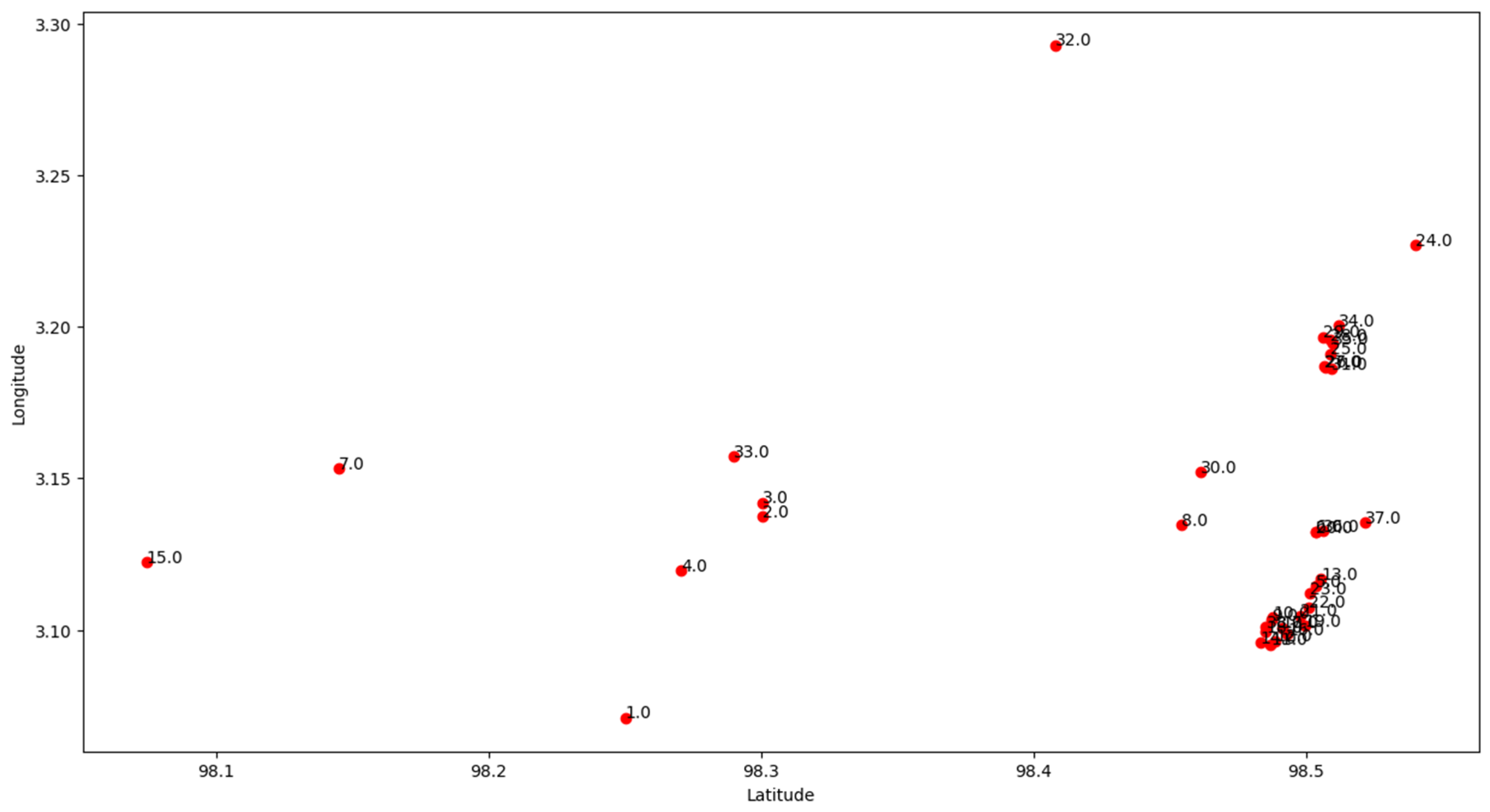
3.1. Numerical Studies

To evaluate the effectiveness of the route formation model in humanitarian logistics, post-disaster demand data will be utilized.

Table 1. Information about demand points.

Demand Point	Latitude	Longitude	Demand
N1	3.071	98.250	2805
N2	3.137	98.301	715
N3	3.142	98.301	366
N4	3.119	98.270	805
N5	3.114	98.504	210
N6	3.132	98.504	122
N7	3.153	98.145	479
N8	3.135	98.454	190
N9	3.103	98.487	386
N10	3.104	98.488	1107
N11	3.095	98.487	415
N12	3.096	98.489	207
N13	3.117	98.505	81
N14	3.096	98.483	1095
N15	3.122	98.074	736
N16	3.099	98.493	503
N17	3.101	98.491	221
N18	3.099	98.485	650
N19	3.101	98.500	258
N20	3.132	98.504	232
N21	3.105	98.498	805
N22	3.108	98.501	1970
N23	3.112	98.502	1136
N24	3.227	98.540	385
N25	3.191	98.509	243
N26	3.187	98.507	637
N27	3.187	98.507	748
N28	3.196	98.509	173
N29	3.197	98.506	535
N30	3.152	98.461	1549
N31	3.186	98.509	1103
N32	3.293	98.408	516
N33	3.157	98.290	1192
N34	3.200	98.512	767
N35	3.194	98.510	1046
N36	3.133	98.506	311
N37	3.135	98.522	534
N38	3.101	98.485	283

provides details regarding the disaster requests, which include 38 shelter posts accommodating a total of 25,516 victims. These requests originate from four sub-districts and 26 villages. The information in Table 1 serves as a basis for assessing the performance and efficiency of the route formation model in addressing the post-disaster demands.

The objective of this study was to develop an allocation model using the k-means clustering machine learning algorithm, and to establish transportation routes in humanitarian logistics using the deep learning approach of Artificial Neural Networks (ANN). The proposed allocation model aims to determine the optimal locations for opening distribution centers in disaster areas, considering uncertain demand points that arise after the disaster. In addition to identifying the locations of newly opened distribution centers, the allocation model also classifies demand points based on their assigned distribution centers. The results of the allocation model are then utilized to create a model for establishing transportation routes in humanitarian logistics.

Table 1 provides an overview of the distribution of 38 demand points following the disaster, including their respective latitude ($x$) and longitude ($y$) coordinates. The geographic distribution of these demand points can be observed in Figure 4, which visually presents their spatial distribution across the affected area.

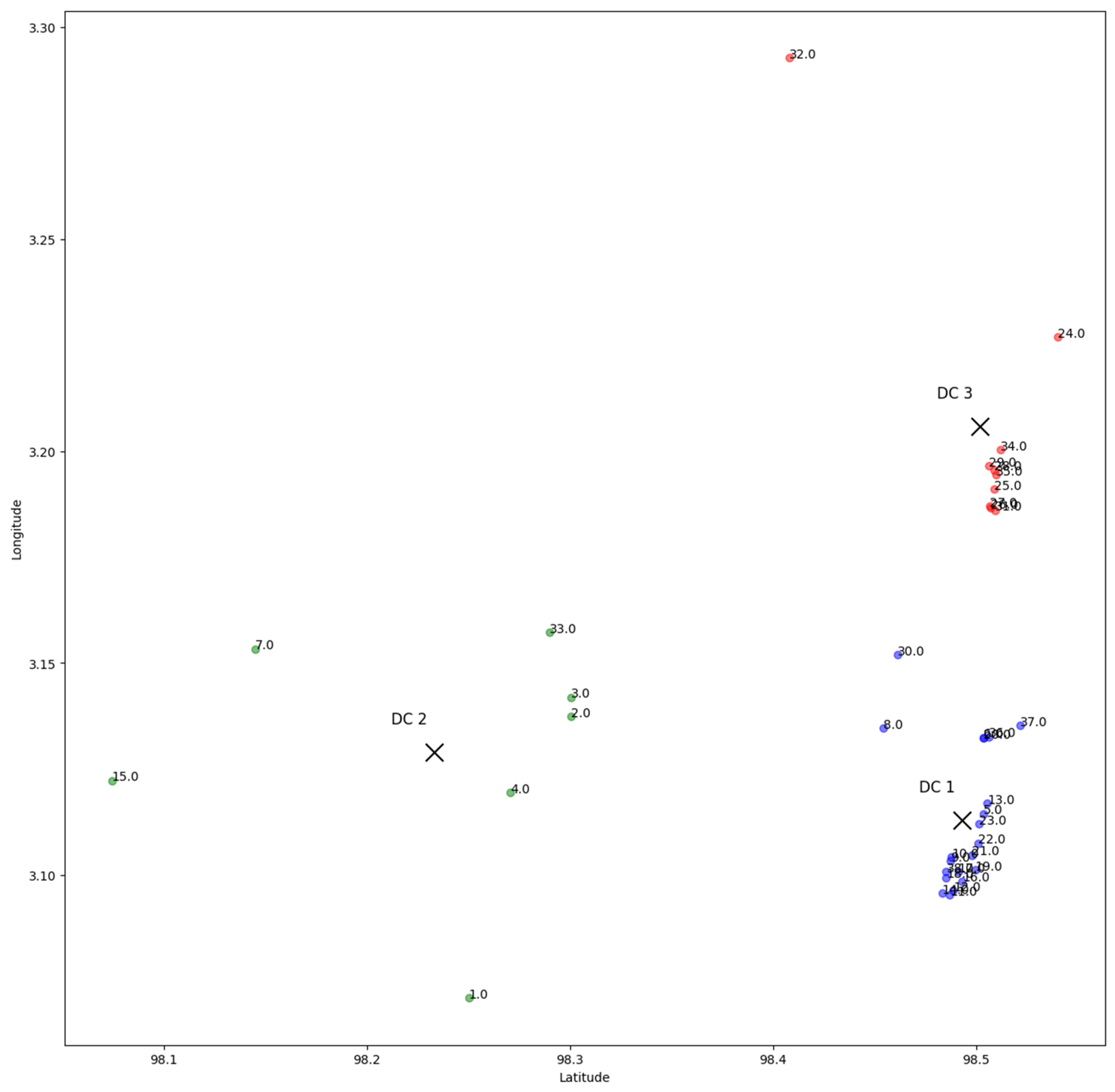
3.2. Clustering Demand Points and Distribution Center Locations

According to Table 1, there were a total of 38 demand points following the disaster. The coordinates of these points were collected and used as input for the K-means technique. Four initial centroids were randomly selected to represent the distribution of demand points. These centroids were derived from four shelter posts.

The K-means algorithm was applied to calculate the distance between each query point and the initial centroid. Based on this distance calculation, each point was assigned to the cluster that was closest to it. This process was repeated for each new cluster formed. To refine the clusters further, each existing cluster was divided into two by utilizing the two most distant demand points within it. This led to the creation of new clusters.

Figure 5 illustrates the results of the grouping process, showcasing the clusters formed based on the assigned distribution center $i$. Through 1000 iterations of optimization, the algorithm determined the optimal location of the distribution center and the grouping of demand points based on this center. The resulting coordinates of the new cluster centroid can be found in

Table 2. Optimal distribution center and demand point grouping.

Distribution Center	Latitude	Longitude	Demand Point
DC1	98.232	3.129	N5, N6, N8, N9, N10, N11, N12, N13, N14, N16, N17, N18, N19, N20, N21, N22, N23, N30, N36, N37, and N38
DC2	98.493	3.103	N1, N2, N3, N4, N7, N15, and N33
DC3	98.492	3.137	N24, N25, N26, N27, N28, N29, N31, N32, N34, and N35

.

An analysis of the number of clusters ($k$) was conducted using the elbow method to determine the optimal number of clusters based on the location data of 38 demand points. This analysis aims to identify the most suitable number of clusters, which will serve as potential candidates for opening distribution centers.

The elbow method was employed to determine the optimal number of clusters based on the location data of 38 demand points. This method helps identify the most suitable number of clusters for opening distribution centers. Figure 6 depicts the graphical representation of the sum of squared distances for different numbers of clusters, highlighting the points of significant bends or decreases. This point indicates the optimal number of clusters to be considered for distribution center openings.

In K-means clustering, determining the optimal number of groups $K$ is an important consideration. The elbow method is a popular approach for assisting in this determination. It utilizes the total within sum of squares (WSS) as a criterion for identifying the optimal $K$. Figure 7 demonstrates this method, showing a sharp change in the line resembling an elbow near the minimum value when $K=3$. Hence, according to the elbow method, the optimal $K$ is achieved at $K=3$.

3.3. Location Prediction and Formation of Distribution Routes

The location prediction model in this study utilizes a deep learning approach with an artificial neural network (ANN) algorithm. The model is trained using data generated from an emergency facility location model that includes three open distribution centers and 38 demand points. Its purpose is to predict the location of the assigned distribution center based on the geographic coordinates of newly opened demand points. By inputting the coordinates of these new demand points into the model, it can accurately predict the corresponding location of the assigned distribution center. This predictive capability aids in efficient and effective decision making for logistics planning in humanitarian operations.

The model training results, as shown in Figure 8, indicate that the model achieves an impressive accuracy rate of 96.15% after 50 epochs. This high accuracy demonstrates that the model has effectively learned from the training data and can make accurate predictions. The accuracy rate gradually increases with each epoch, indicating that the model continuously improves its internal parameters to enhance its performance. With such a high accuracy rate of 96.15%, the model holds significant potential for reliable predictions, and can be effectively applied in various contexts, including location prediction and data classification tasks.

3.4. Formation of Distribution Routes

Three distribution centers (DC) $i$ will be determined from the 38 demand points, with 21 demand points in the ${DC}_1$ cluster, 7 demand points in the ${DC}_2$ cluster, and 10 demand points in the ${DC}_3$ cluster. These outcomes serve as the input layer $\left(X_1,\dots ,X_n\right)$ in the construction of transportation routes. Using Equations (5) to (6), the hidden layer uses the distribution of the location of the request point $\left(L_{11},\dots ,L_{ij}\right)$ to produce an output layer; namely, the route $\left(Y_1,\dots ,Y_n\right)$.

Table 3. Results of establishing distribution routes with deep learning.

Distribution Center	Number of Distribution Centers	Number of Demand Points	Vehicles	Route Combinations	Route Selection
DC1	1	21	4	387,467,405	363,626
DC2	1	7	2	3.129	122
DC3	1	10	4	514	50
Total route combinations		387,471,048		363,798

shows the results of using the deep learning model approach to form distribution routes.

For small networks, off-the-shelf software such as CPLEX can solve the problem. The problem cannot be solved as the network size grows, and it is demonstrated that when the number of request points exceeds 11, CPLEX cannot solve the problem on personal computers due to insufficient memory, demonstrating the need for a metaheuristic algorithm. To test the deep route planning (DRP) model’s performance in constructing the proposed route, we extracted a small network from the network shown in Figure 7 and ran experiments to compare route formation results using permutations and deep learning models. The network consists of four candidate DCs, 38 demand points (numbered 1 through 38), and ten vehicles. All tests were performed using Python code on a computer with an Intel Core i5-8250U 1.60 GHz CPU and 8 GB RAM.

Table 4. Comparison of the number of routes generated.

Distribution Center	Number of Distribution Centers	Number of Demand Points	Demand	Vehicles	Exact	DLRP
					Route Combinations	Route Combinations	Route Selection
DC1	1	21	5.225	4	5.10909 × 1019	387,467,405	363,626
DC2	1	7	7.417	2	5040	3129	122
DC3	1	10	5.038	4	3,628,800	514	50
Route formation					5.10909 × 1019	387,471,048	363,798

summarizes the findings.

Table 4 shows that DLRP was able to obtain fewer routes than permutation theory for all networks in DC. The results of route formation in the transportation network with 3 DC candidates, 38 demand points, and 10 vehicles assigned in the network, are that the permutation theory produces 5.10909E+19 and the DLRP model produces 387,471,048 combined routes, where route selection will be performed with 363,798 routes. By reducing the number of route formation results, computation time is reduced, allowing the model to be used in real-world situations such as when a disaster occurs, requiring quick decisions and strategies based on large-scale data in humanitarian logistics.

3.5. Optimal Route

A route model for the distribution of relief goods will be included from the route generated in order to determine the time and cost of distributing the relief goods.

Distribution Centre 1 (DC1) with combination route DC1 → N6 → N20 → N36 → N37 → DC1 with total demand 2.431.

$$\begin{array}{ll}j& =6.9DC1N6+3N 6N 20+0.28N 20N 36+12.6N 36N 37+16.1N 37DC1\\ & =38.88 \mathrm{km}\\ w& =6.9DC1N6+3N 6N 20+0.28N 20N 36+12.6N 36N 37+16.1N 37DC1\\ & =84 \min \\ h& =2000DC1+\left(3.5\ast \left(6.9DC1N6+3N6N20+0.28N20N36+12.6N36N37+16.1N37DC1\right)+500K1DC1\right)\\ & \hspace{1em}\hspace{1em}\hspace{1em}\hspace{1em}\hspace{1em}+0\mathrm{route}1DC1+0\mathrm{route}1DC1\\ & =2000+136.08+500+0+0\\ & =2636.08\end{array}$$

Time ($w$) and cost ($h$) are generated based on route 1 (DC1 → 6.0 → 20.0 → 36.0 → 37.0 → DC1) based on the bi-objective model, so the sum weighted method is used to change it to a single objective model by proposing $\gamma$ weighting parameters. The model generated by ${\overline{P}}_1$ using Equation (17) is a single-objective mixed integer linear programming problem that can be solved using existing commercial problem solvers.

The objective function will be produced by the time parameter (set weighting $\gamma =1$) and the cost parameter (parameter weighting $\gamma =0$):

$$\begin{array}{ll}\mathrm{Minimum} {\overline{\mathcal{z}}}_1\left(\mathrm{route}1\right)& \text{= 1 × 54 route1DC1 + (1 − 0) 2645.00 route1DC1}\\ & \text{= 54 + 264500}\\ & \text{= 2.69900}\end{array}$$

Table 5. The objective function of the optimal route.

No. of Routes	Normal Route			Forbidden Route
	$\mathbf{Time} (\mathit{w}$)	$\mathbf{Cost} (\mathit{h}$)	${\overline{\mathit{P}}}_1$	$\mathbf{Time} (\mathit{w}$)	$\mathbf{Cost} (\mathit{h}$)	${\overline{\mathit{P}}}_1$
1	54	2645.00	2699.00	54	2645.00	2699.00
2	87	2627.26	2714.26	87	2627.26	2714.26
3	58	2583.30	2641.30	58	2583.30	2641.30
4	49	2643.52	2692.52	49	2643.52	2692.52
5	118	1824.80	1942.80	139	1829.60	1968.60
6	289	1943.80	2232.80	289	1943.80	2232.80
7	43	1629.68	1672.68	43	1629.68	1672.68
8	181	1460.40	1641.40	181	1460.40	1641.40
9	58	1270.20	1328.20	58	1270.20	1328.20
10	32	1627.41	1659.41	32	1627.41	1659.41
Total	969	20,255.37	21,224.37	990	20,260.17	21,250.17

shows a single objective function (${\overline{P}}_1$) based on the route recommendations generated, with a total of 38 demand points and 3 distribution centers based on the above calculations.

3.6. Optimal Route with Forbidden Route

A forbidden route is one that cannot be passed or taken due to limitations or constraints. These constraints or impediments can take the form of policies or regulations imposed by related parties, geographical or topographical conditions, or other factors that prevent certain routes from being traversed. Prohibited routes can have an impact on the efficiency and effectiveness of shipping because they limit the routes that can be chosen and necessitate special strategies to avoid them in logistics or transportation problems. As a result, modeling and managing prohibited routes is critical in logistics and transportation planning and management. Following the completion of route modeling, it is necessary to check and inspect prohibited routes that must be avoided when delivering disaster relief goods. Given a set of prohibited routes on route location id 3 to location id 33 ($3\nRightarrow 33$) or vice versa—location id 33 to location id 33 ($33\nRightarrow 3$)—every node on each route formed will be checked regarding whether it is passing through a forbidden route or a non-forbidden route. The results of using the distribution route model with forbidden routes from DC2 with a total of 7 request locations are 122 route combinations; with a set of routes that cannot be traversed, namely ($3\nRightarrow 33$) and ($33\nRightarrow 3$), the result is 48 prohibited routes and 74 non-prohibited routes.

To find the optimal route, it has to be based on routes that have been declared not to be a group of non-prohibited routes, namely routes that do not contain the sets $\left\{3\right\}$ and $\left\{33\right\}$, namely $\left\{\mathrm{3,33}\right\}$ or $\left\{\mathrm{33,3}\right\}$, totaling 74 routes. A route model for the distribution of aid goods will be included from the non-prohibited routes generated to find the time and cost of distributing aid goods.

DC2 cluster 2 with combination route DC2 → N4 → N33 → N2 → N3 → N1 → DC2 with total demand 2431:

$$\begin{array}{ll}j& =7.1DC2N4+6.9N4N33+4.5N33N2+2N2N3+17.4N3N1+17N1DC2\\ & =57.4 \mathrm{km}\\ w& =615DC2N4+18N4N33+10N33N2+25N2N3+36N3N1+32N1DC2\\ & =139 \min \\ h& =1000DC2+\left(4\ast \left(7.1DC2N4+6.9N4N33+4.5N33N2+2N2N3+17.4N3N1+17N1DC2\right)\right)\\ & \hspace{1em}\hspace{1em}\hspace{1em}\hspace{1em}\hspace{1em}+600K1DC1+0route1DC1+0route1DC1\\ & =1000+229.6+600+0+0\\ & =1829.6\end{array}$$

Based on the aforementioned calculations, the objective function aims to minimize both time and cost, taking into account the prohibited routes, specifically {3} and {33} (denoted as {3,33} or {33,3}). The results of the objective function, considering both the normal route and the forbidden route, are presented in Table 5. This table provides insights into the achieved values for time and cost when comparing the optimal routes generated by these two models. By analyzing the values in this table, we can assess the effectiveness of the forbidden route model in minimizing both time and cost while avoiding the specified forbidden routes.

Table 3 provides a comparison between the normal route model and the forbidden route model. The difference between the two models is observed in route 5, where the forbidden route model excludes the path {3,33} or {33,3}, as it is a forbidden path.

Consequently, in the forbidden route model, this particular route is avoided, and an alternative route is selected that avoids the forbidden path. As a result, there is an increase in both time $\left(w\right)$ and cost $\left(h\right)$ for route 5, with a time increase of 0.02167 and a cost increase of 0.00024. This demonstrates that if a route contains a forbidden or impassable path, there will be an associated increase in both time and cost.

The optimal route can be visually represented using the graphical depiction shown in Figure 9, Figure 10 and Figure 11, illustrating the optimized route for the given problem.

The route for the distribution of disaster relief goods, as depicted in Figure 9, Figure 10 and Figure 11, consists of three distribution centers (DCs) and 38 demand points. This arrangement leads to the identification of ten optimal routes, which serve as a reference for vehicles tasked with distributing relief goods to the 38 demand point locations. The top ten optimal routes are as follows:

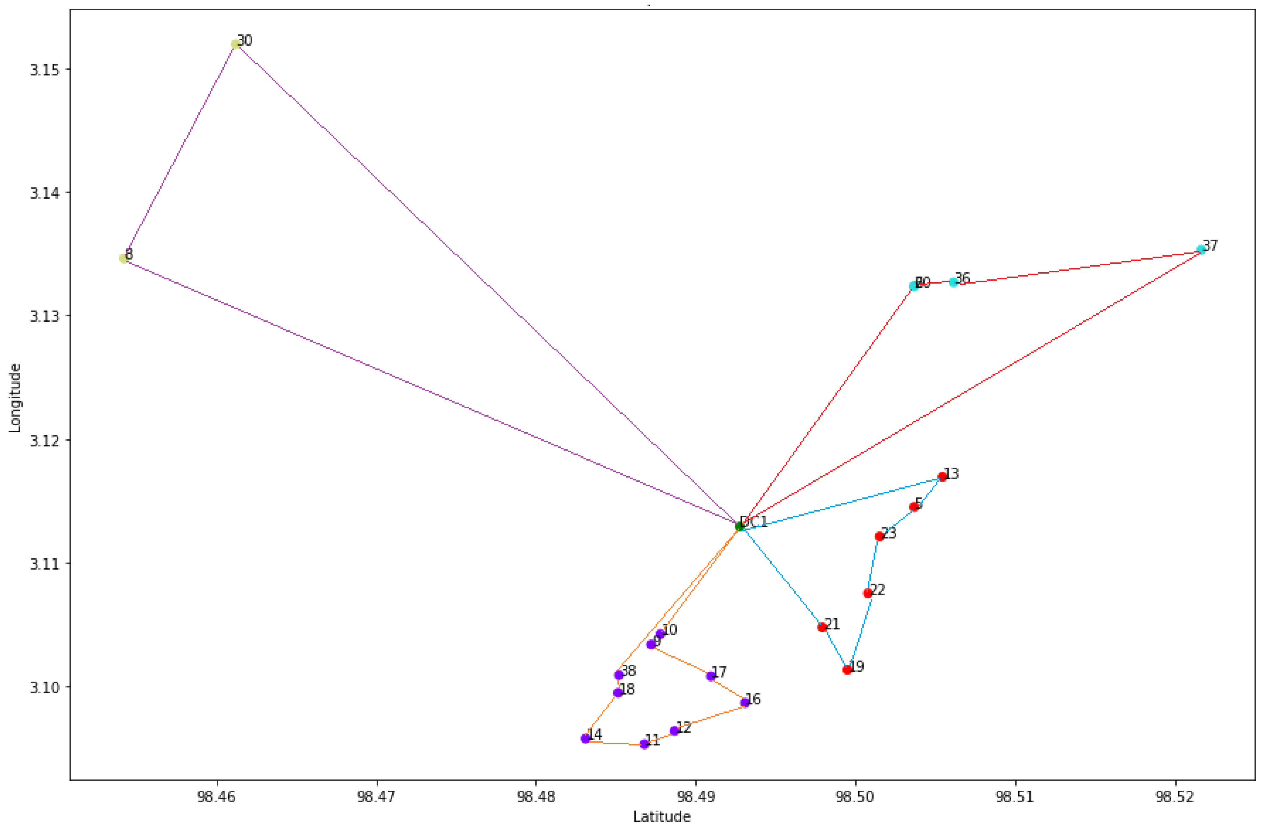
• Route 1: DC1 → 19 → 13 → 5 → 23 → 22 → 21 → DC1
• Route 2: DC1 → 6 → 36 → 20 → 37 → DC1
• Route 3: DC1 → 30 → 8 → DC1
• Route 4: DC1 → 9 → 10 → 12 → 11 → 18 → 38 → 16 → 14 → 17 → DC1
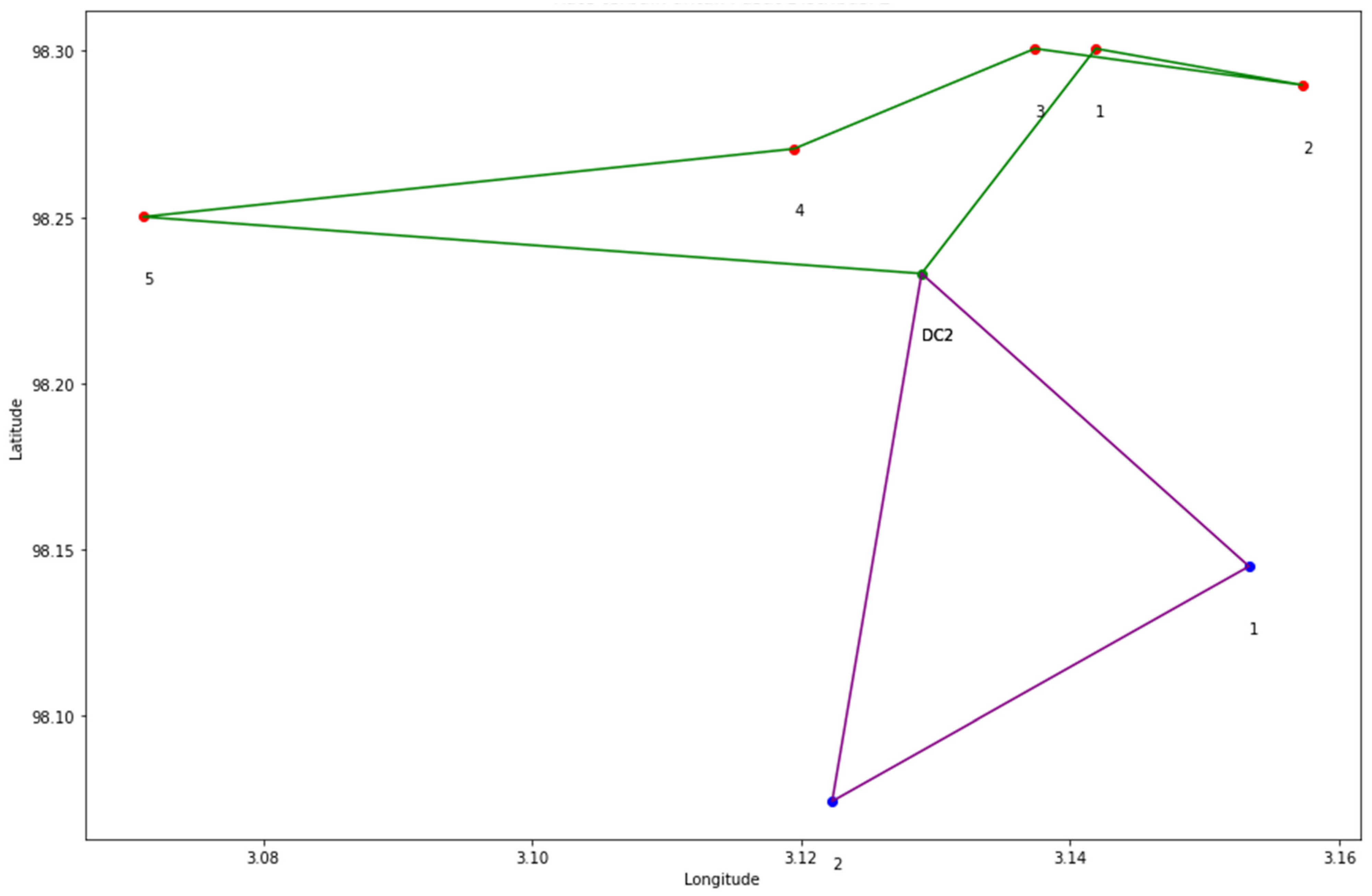
• Route 5: DC2 → 3 → 33 → 2 → 4 → 10 → DC2
• Route 6: DC2 → 7 → 15 → DC2
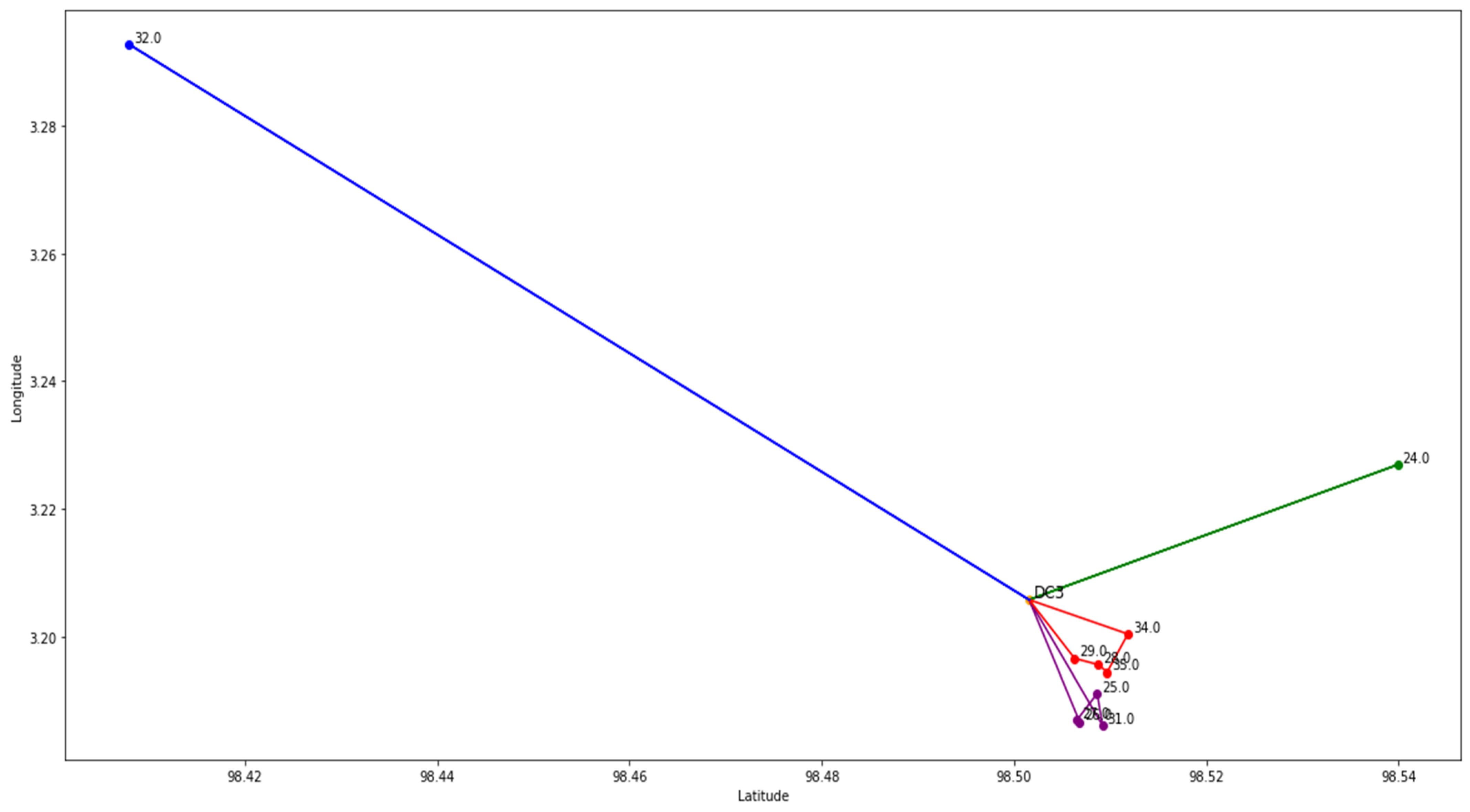
• Route 7: DC3 → 34 → 35 → 28 → 29 → DC3
• Route 8: DC3 → 32 → DC3
• Route 9: DC3 → 24 → DC3
• Route 10: DC3 → 31 → 25 → 27 → 26 → DC3

4. Conclusions

In conclusion, this paper introduces the deep location routing problem (DLRP) model as an innovation in route planning within the context of disaster logistics. The DLRP model is specifically designed to address the challenges associated with the location routing problem (LRP), which is a key issue in distributing humanitarian aid after disasters. DLRP utilizes the K-means algorithm to determine optimal facility locations, which is a critical step in ensuring efficient distribution centers closely linked to post-disaster rescue and recovery efforts. Furthermore, DLRP harnesses artificial intelligence in the form of artificial neural networks (ANN) within the deep learning model for route prediction and planning. This allows for responsive and adaptive route planning, even in uncertain or changing conditions. One of the major advantages of the DLRP model is its ability to efficiently tackle NP-hard problems, yielding optimal solutions with polynomial time complexity. This means that disaster relief distribution can be carried out more effectively and responsively, with more efficient resource utilization. In the context of disaster logistics, where every second is precious, the DLRP model holds significant potential to enhance preparedness and disaster response capabilities. With the existence of this model, disaster logistics management can become more efficient, timely, and adaptive, thereby helping to reduce the impact on human suffering and property loss in emergency situations. As a result, this research opens the door to further improvements in disaster management and humanitarian aid distribution worldwide.

Further research in this topic could explore several areas. One area of focus could be the development of more complex and realistic models that consider a wider range of variables and constraints that may arise in disaster logistics management. Additionally, further research could investigate the practical implementation of the deep location routing problem (DLRP) model in real-world scenarios and assess its impact on operational efficiency and responsiveness in actual disaster situations. Furthermore, research into the integration of emerging technologies such as the Internet of Things (IoT) and big data processing in the context of disaster logistics management could also be an intriguing area to explore. By continuing to emphasize research and development in this field, we can enhance our preparedness and response to disasters and reduce their impact on affected communities.

References

1. Ma, K.; Yan, H.; Ye, Y.; Zhou, D.; Ma, D. Critical Decision-Making Issues in Disaster Relief Supply Management: A Review. Comput. Intell. Neurosci. 2022, 2022, 1105839. [Google Scholar] [CrossRef]
2. Roh, S.; Lin, H.H.; Jang, H. Performance Indicators for Humanitarian Relief Logistics in Taiwan. Asian J. Shipp. Logist. 2022, 38, 173–180. [Google Scholar] [CrossRef]
3. Lu, Q.; Goh, M.; De Souza, R. A SCOR Framework to Measure Logistics Performance of Humanitarian Organizations. J. Humanit. Logist. Supply Chain Manag. 2016, 6, 222–239. [Google Scholar] [CrossRef]
4. Mohd, S.; Fathi, M.S.; Harun, A.N.; Omar Chong, N. Key issues in the management of the humanitarian aid distribution process during and post-disaster in malaysia. Plan. Malays. J. 2018, 16, 211–221. [Google Scholar] [CrossRef]
5. Dahiya, C.; Sangwan, S. Literature Review on Travelling Salesman Problem. Int. J. Res. 2018, 5, 1152–1155. [Google Scholar]
6. Nadizadeh, A. Formulation and a Heuristic Approach for the Orienteering Location-Routing Problem. RAIRO Oper. Res. 2021, 55, S2055–S2069. [Google Scholar] [CrossRef]
7. Safari, F.M.; Etebari, F.; Chobar, A.P. Modeling and Optimization of a Tri-Objective Transportation-Location-Routing Problem Considering Route Reliability: Using MOGWO, MOPSO, MOWCA, and NSGA-II. J. Optim. Ind. Eng. 2021, 14, 83–98. [Google Scholar] [CrossRef]
8. Zhong, S.; Cheng, R.; Jiang, Y.; Wang, Z.; Larsen, A.; Nielsen, O.A. Risk-Averse Optimization of Disaster Relief Facility Location and Vehicle Routing under Stochastic Demand. Transp. Res. Part E Logist. Transp. Rev. 2020, 141, 102015. [Google Scholar] [CrossRef]
9. Rahbari, M.; Arshadi Khamseh, A.; Sadati-Keneti, Y.; Jafari, M.J. A Risk-Based Green Location-Inventory-Routing Problem for Hazardous Materials: NSGA II, MOSA, and Multi-Objective Black Widow Optimization. Environ. Dev. Sustain. 2022, 24, 2804–2840. [Google Scholar] [CrossRef]
10. Peng, Z.; Wang, C.; Xu, W.; Zhang, J. Research on Location-Routing Problem of Maritime Emergency Materials Distribution Based on Bi-Level Programming. Mathematics 2022, 10, 1243. [Google Scholar] [CrossRef]
11. Cheng, C.; Thompson, R.G.; Costa, A.M.; Huang, X. Application of the Bi-Level Location-Routing Problem for Post-Disaster Waste Collection. In City Logistics 2; Wiley: Hoboken, NJ, USA, 2018. [Google Scholar] [CrossRef]
12. Liu, C.; Kou, G.; Peng, Y.; Alsaadi, F.E. Location-Routing Problem for Relief Distribution in the Early Post-Earthquake Stage from the Perspective of Fairness. Sustainability 2019, 11, 3420. [Google Scholar] [CrossRef]
13. Shen, L.; Tao, F.; Shi, Y.; Qin, R. Optimization of Location-routing Problem in Emergency Logistics Considering Carbon Emissions. Int. J. Environ. Res. Public Health 2019, 16, 2982. [Google Scholar] [CrossRef] [PubMed]
14. Wang, S.; Tao, F.; Shi, Y. Optimization of Location–Routing Problem for Coldchain Logistics Considering Carbon Footprint. Int. J. Environ. Res. Public Health 2018, 15, 86. [Google Scholar] [CrossRef] [PubMed]
15. Wei, X.; Qiu, H.; Wang, D.; Duan, J.; Wang, Y.; Cheng, T.C.E. An Integrated Location-Routing Problem with Post-Disaster Relief Distribution. Comput. Ind. Eng. 2020, 147, 106632. [Google Scholar] [CrossRef]
16. Wang, D.; Yang, K.; Yang, L.; Li, S. Distributional Robustness and Lateral Transshipment for Disaster Relief Logistics Planning under Demand Ambiguity. Int. Trans. Oper. Res. 2022. online ahead of print. [Google Scholar] [CrossRef]
17. Abazari, S.R.; Aghsami, A.; Rabbani, M. Prepositioning and Distributing Relief Items in Humanitarian Logistics with Uncertain Parameters. Socio-Econ. Plan. Sci. 2021, 74, 100933. [Google Scholar] [CrossRef]
18. Zhan, S.L.; Liu, S.; Ignatius, J.; Chen, D.; Chan, F.T.S. Disaster Relief Logistics under Demand-Supply Incongruence Environment: A Sequential Approach. Appl. Math. Model. 2021, 89, 592–609. [Google Scholar] [CrossRef]
19. Aghajani, M.; Torabi, S.A.; Heydari, J. A Novel Option Contract Integrated with Supplier Selection and Inventory Prepositioning for Humanitarian Relief Supply Chains. Socio-Econ. Plan. Sci. 2020, 71, 100780. [Google Scholar] [CrossRef]
20. Maharjan, R.; Hanaoka, S. A Credibility-Based Multi-Objective Temporary Logistics Hub Location-Allocation Model for Relief Supply and Distribution under Uncertainty. Socio-Econ. Plan. Sci. 2020, 70, 100727. [Google Scholar] [CrossRef]
21. Liu, Y.; Cui, N.; Zhang, J. Integrated Temporary Facility Location and Casualty Allocation Planning for Post-Disaster Humanitarian Medical Service. Transp. Res. Part E Logist. Transp. Rev. 2019, 128, 1–16. [Google Scholar] [CrossRef]
22. Praneetpholkrang, P.; Huynh, V.N.; Kanjanawattana, S. A Multi-Objective Optimization Model for Shelter Location-Allocation in Response to Humanitarian Relief Logistics. Asian J. Shipp. Logist. 2021, 37, 149–156. [Google Scholar] [CrossRef]
23. Liu, Y.; Yuan, Y.; Shen, J.; Gao, W. Emergency Response Facility Location in Transportation Networks: A Literature Review. J. Traffic Transp. Eng. 2021, 8, 153–169. [Google Scholar] [CrossRef]
24. Gizaw, B.T.; Gumus, A.T. Humanitarian Relief Supply Chain Performance Evaluation: A Literature Review. Int. J. Mark. Stud. 2016, 8, 105–120. [Google Scholar] [CrossRef]
25. Pouyanfar, S.; Tao, Y.; Tian, H.; Chen, S.C.; Shyu, M.L. Multimodal Deep Learning Based on Multiple Correspondence Analysis for Disaster Management. World Wide Web 2019, 22, 1893–1911. [Google Scholar] [CrossRef]
26. Aqib, M.; Mehmood, R.; Alzahrani, A.; Katib, I. A Smart Disaster Management System for Future Cities Using Deep Learning, Gpus, and in-Memory Computing. In Smart Infrastructure and Applications; EAI/Springer Innovations in Communication and Computing; Springer: Berlin/Heidelberg, Germany, 2020. [Google Scholar] [CrossRef]
27. Alidoost, F.; Arefi, H. Application of Deep Learning for Emergency Response and Disaster Management. In Proceedings of the AGSE Eighth International Summer School and Conference, Tehran, Iran, 29 April–4 May 2017; Iran University of Tehran: Tehran, Iran, 2017; pp. 11–17. [Google Scholar]
28. Aqib, M.; Mehmood, R.; Albeshri, A.; Alzahrani, A. Disaster Management in Smart Cities by Forecasting Traffic Plan Using Deep Learning and GPUs. In Smart Societies, Infrastructure, Technologies and Applications; Lecture Notes of the Institute for Computer Sciences, Social-Informatics and Telecommunications Engineering, LNICST; Springer: Berlin/Heidelberg, Germany, 2018; Volume 224. [Google Scholar] [CrossRef]
29. Yi, Y.; Zhang, W. A New Deep-Learning-Based Approach for Earthquake-Triggered Landslide Detection from Single-Temporal RapidEye Satellite Imagery. IEEE J. Sel. Top. Appl. Earth Obs. Remote Sens. 2020, 13, 6166–6176. [Google Scholar] [CrossRef]
30. Antoniou, V.; Potsiou, C. A Deep Learning Method to Accelerate the Disaster Response Process. Remote Sens. 2020, 12, 544. [Google Scholar] [CrossRef]
31. Galera-Zarco, C.; Floros, G. A Deep Learning Approach to Improve Built Asset Operations and Disaster Management in Critical Events: An Integrative Simulation Model for Quicker Decision Making. Ann. Oper. Res. 2023, 1–40. [Google Scholar] [CrossRef]
32. Devaraj, J.; Ganesan, S.; Elavarasan, R.M.; Subramaniam, U. A Novel Deep Learning Based Model for Tropical Intensity Estimation and Post-Disaster Management of Hurricanes. Appl. Sci. 2021, 11, 4129. [Google Scholar] [CrossRef]
33. Panahi, M.; Jaafari, A.; Shirzadi, A.; Shahabi, H.; Rahmati, O.; Omidvar, E.; Lee, S.; Bui, D.T. Deep Learning Neural Networks for Spatially Explicit Prediction of Flash Flood Probability. Geosci. Front. 2021, 12, 101076. [Google Scholar] [CrossRef]
34. Bragagnolo, L.; da Silva, R.V.; Grzybowski, J.M.V. Landslide Susceptibility Mapping with r.Landslide: A Free Open-Source GIS-Integrated Tool Based on Artificial Neural Networks. Environ. Model. Softw. 2020, 123, 104565. [Google Scholar] [CrossRef]
35. Zhang, Y.; Hao, Y. Loss Prediction of Mountain Flood Disaster in Villages and Towns Based on Rough Set RBF Neural Network. Neural Comput. Appl. 2022, 34, 2513–2524. [Google Scholar] [CrossRef]
36. Pathirana, D.; Chandrasiri, L.; Jayasekara, D.; Dilmi, V.; Samarasinghe, P.; Pemadasa, N. Deep Learning Based Flood Prediction and Relief Optimization. In Proceedings of the 2019 International Conference on Advancements in Computing, ICAC 2019, Malabe, Sri Lanka, 5–6 December 2019. [Google Scholar] [CrossRef]
37. Khosla, E.; Ramesh, D.; Sharma, R.P.; Nyakotey, S. RNNs-RT: Flood Based Prediction of Human and Animal Deaths in Bihar Using Recurrent Neural Networks and Regression Techniques. Procedia Comput. Sci. 2018, 132, 486–497. [Google Scholar] [CrossRef]
38. Gupta, M.K.; Chandra, P. Effects of Similarity/Distance Metrics on k-Means Algorithm with Respect to Its Applications in IoT and Multimedia: A Review. Multimed. Tools Appl. 2022, 81, 37007–37032. [Google Scholar] [CrossRef]
39. Moshref-Javadi, M.; Lee, S. The Latency Location-Routing Problem. Eur. J. Oper. Res. 2016, 255, 604–619. [Google Scholar] [CrossRef]
40. Pratiwi, A.B.; Sasmito, A.; Istiqomah, Q.S.; Kurniawan, M.R.; Suprajitno, H. Metaheuristic Algorithms for Solving Multiple-Trips Vehicle Routing Problem with Time Windows (MTVRPTW). J. Phys. Conf. Ser. 2019, 1306, 012021. [Google Scholar] [CrossRef]
Figure 1. Diagram of the formation of transportation routes in post-disaster areas for humanitarian logistics.
Algorithms 16 00468 g001
Figure 2. Schematic of the model for forming transportation routes based on deep learning.
Algorithms 16 00468 g002
Figure 3. Design of an emergency facility location model.
Algorithms 16 00468 g003
Figure 4. Model for designing routes based on deep learning.
Algorithms 16 00468 g004
Figure 5. Demand point locations.
Algorithms 16 00468 g005
Figure 6. Grouping demand points into clusters (distribution centers) using geographic coordinates (latitude, longitude).
Algorithms 16 00468 g006
Figure 7. Elbow graphic.
Algorithms 16 00468 g007
Figure 8. Predictive model training graph.
Algorithms 16 00468 g008
Figure 9. Graph of optimal relief goods distribution route at DC1.
Algorithms 16 00468 g009
Figure 10. Graph of optimal relief goods distribution route at DC2.
Algorithms 16 00468 g010
Figure 11. Graph of optimal relief goods distribution routes at DC3.
Algorithms 16 00468 g011