Article

Comparison of Different Radial Basis Function Networks for the Electrical Impedance Tomography (EIT) Inverse Problem

1
Department of Physics, Shahjalal University of Science and Technology, 3100 Sylhet, Bangladesh
2
Department of Mathematics, Shahjalal University of Science and Technology, 3114 Sylhet, Bangladesh
3
ETAS Research, Robert Bosch GMBH, 70469 Stuttgart, Germany
4
Department of Mathematics and Statistics, UNC Charlotte, Charlotte, NC 28223, USA
*
Author to whom correspondence should be addressed.
Algorithms 2023, 16(10), 461; https://doi.org/10.3390/a16100461
Submission received: 20 August 2023 / Revised: 25 September 2023 / Accepted: 26 September 2023 / Published: 28 September 2023

Abstract

:
This paper aims to determine whether regularization improves image reconstruction in electrical impedance tomography (EIT) using a radial basis network. The primary purpose is to investigate the effect of regularization to estimate the network parameters of the radial basis function network to solve the inverse problem in EIT. Our approach to studying the efficacy of the radial basis network with regularization is to compare the performance among several different regularizations, mainly Tikhonov, Lasso, and Elastic Net regularization. We vary the network parameters, including the fixed and variable widths for the Gaussian used for the network. We also perform a robustness study for comparison of the different regularizations used. Our results include (1) determining the optimal number of radial basis functions in the network to avoid overfitting; (2) comparison of fixed versus variable Gaussian width with or without regularization; (3) comparison of image reconstruction with or without regularization, in particular, no regularization, Tikhonov, Lasso, and Elastic Net; (4) comparison of both mean square and mean absolute error and the corresponding variance; and (5) comparison of robustness, in particular, the performance of the different methods concerning noise level. We conclude that by looking at the R2 score, one can determine the optimal number of radial basis functions. The fixed-width radial basis function network with regularization results in improved performance. The fixed-width Gaussian with Tikhonov regularization performs very well. The regularization helps reconstruct the images outside of the training data set. The regularization may cause the quality of the reconstruction to deteriorate; however, the stability is much improved. In terms of robustness, the RBF with Lasso and Elastic Net seem very robust compared to Tikhonov.

1. Introduction

The distribution of electrical conductivity permittivity, or the impedance of biological structures, varies. For example, there is a contrast in electrical properties between tumorous versus non-tumorous tissue. Therefore, the conductivity distribution contains valuable information to identify whether in-homogeneity exists, such as a tumor in biological tissue. Electrical impedance tomography (EIT) is used to construct an image of these electrical properties inside biological tissue. EIT has been applied to detect pulmonary emboli [1,2] and breast cancer [1] and to monitor apnoea [3], heart function, and blood flow [4]. EIT also has many non-medical applications, such as locating minerals [5], oil extractions from underground [6], and detecting corrosion [7] and minor defects in metals [8,9].
In EIT, the image is reconstructed by measuring the boundary current and voltage using several electrodes placed on the surface. This gives the Neumann to Dirichlet (NtD) map, which is then used to work backward and find the conductivity in the domain. This is the EIT inverse problem. There are many technical problems related to EIT image reconstruction, such as finding the best arrangement of electrode positions [10], seeing the impact of boundary surface and electrode contact [11], hardware development [12], a stable reconstruction algorithm, and much more. The EIT inverse problem is known to be highly nonlinear and exponentially ill posed. Here, we focus mainly on solving the inverse problem mathematically without investigating the practical issues associated with EIT imaging. To solve the inverse problem in the machine learning setting, one must solve the forward problem, which involves finding the NtD map from a given conductivity. This is also useful for the verification of the inverse solution. In our case, this is used for generating the training data for the neural network. There are a few analytical solutions to the forward problem for some selected configurations [13,14]. This work solves the two-dimensional forward problem using the finite element method to generate the training data.
The inverse problem of the EIT image reconstruction was first introduced by Calderón [15]. As formulated by Calderón, the inverse problem is to retrieve the conductivity σ from the NtD map Λ σ . It is well known that under various assumptions and smoothness for the conductivity, a unique solution to the Calderón problem exists [16]. In particular, for the 2D case, it has been shown that a unique solution exists even with very minimal smoothness assumptions on the conductivity [17]. Furthermore, the two-dimensional Calderón problem is stable when the conjunctivitis is Hölder-continuous [18]. Another practical issue is that complete boundary data are never practically measured. We only measure partial data, affecting the inverse solution’s accuracy. The uniqueness of the Calderón problem in the 2D case with partial data has also been found under certain conditions [19,20]. We simulate synthetic data using a complete electrode model in our numerical experiments to represent EIT measurements accurately.
The radial basis function (RBF) network has been proposed as a machine learning approach using neural networks to represent nonlinear functions. There exist papers by several authors [21,22,23,24,25,26] that solve the EIT inverse problem using the radial basis function. Some authors used a radial basis function with a Gaussian activation function where the Gaussian width factor is different for each radial basis function in the hidden layer [21,22,23,24], while others use the same width for all the Gaussian functions [25,26]. It is not immediately clear which of these two models performs better as there have been no comparison studies to the best of our knowledge. In this manuscript, we mainly focus on the impact of regularization for the RBF, but not on the classical methods. We demonstrate our approach using synthetic data for proof of concept as it is an important and first step. This is because in practice, we would still need to train the RBF network with simulated data before applying the model to experimental data. We mainly focus on the numerical and mathematical aspect of the EIT inverse reconstruction using the RBF network for this work.

1.1. Significance of the Work

It is well known that regularization for the EIT inverse problem is essential for obtaining proper and stable reconstructions. We investigate methodically the implementation of RBF for EIT with or without regularization, and demonstrate that regularization is required for optimal performance. However, to our knowledge, no prior work has methodically studied the effectiveness of different regularizations for the EIT inverse problems with radial basis function networks. In this paper, we use numerical simulations to (1) determine the optimal number of radial basis functions in the network to avoid overfitting; (2) compare the fixed versus variable Gaussian width with or without regularization; (3) compare image reconstruction with or without regularization, in particular, no regularization, Tikhonov, Lasso, and Elastic Net; (4) compare both mean square and mean absolute error and the corresponding variance; and (5) compare robustness, in particular, the performance of the different methods concerning noise level. We conclude that by looking at the R 2 score, one can determine the optimal number of radial basis functions. The fixed-width radial basis function network with regularization results in improved performance. The fixed-width Gaussian with Tikhonov regularization performs very well. The regularization helps reconstruct the images outside of the training data set. The regularization may cause the quality of the reconstruction to deteriorate; however, the stability is much improved. In terms of robustness, the RBFs with Lasso and Elastic Net seem very robust compared to Tikhonov.

1.2. Organization of the Paper

The organization of this paper is as follows. Section 2 introduces the continuum model and its primary finite element method (FEM) formulation. Section 2.1 briefly overviews the complete electrode model and its FEM formulation. We use this model to generate our training data. Section 3 explains the radial basis function (rbf) network, the loss functions used, and how we optimized it. In Section 4, we explain how our simulations chose our hyperparameters and show some of the reconstructed images by the different models. Finally, we conclude with closing remarks and possible improvements in Section 5.

2. The Continuum Model for EIT

The primary vector fields in electrodynamics are the electric field E and the magnetic field H . These fields, when applied to a material, produce electric displacement D = ϵ E and magnetic flux B = μ H [27], where ϵ and μ are the electric permittivity and the magnetic permeability, respectively. For a static electric field, E can be written as ϕ [27], where ϕ is then the electric potential. Here, we will work assuming that the electric field is static. The current density at a point is given by J = σ E [27]. σ is the conductivity of the material at that point. In general, σ is a tensor of rank two that can be represented using a 3 × 3 matrix. However, we will assume that σ = σ ( x , y ) I , where I is the identity matrix. The equation of interest in both the EIT forward problem and the inverse problem is found by taking the divergence on both sides of Maxwell’s equation corresponding to Ampere’s law [28]
× H = D t + J
which gives in the static electric field case
· σ ϕ = 0
on a region of space Ω . The forward problem is to find ϕ inside Ω , given σ and the Neumann boundary condition
σ ( x ) ϕ ( x ) · n = σ ( x ) ϕ ( ( x ) n = j ( x ) for x Ω
subject to Ω j ( x ) d s = 0
where n is the outward normal unit vector at Ω , and hence, j is the surface normal component of the current density at the boundary. The Dirichlet boundary value problem has a unique solution [29], at least within the weak sense, assuming that σ m < 0 and σ L ( Ω ¯ ) . The Neumann boundary value problem has a unique solution [29] up to an additive constant, which is fixed by the choice of ground:
Ω V ( x ) d s = 0
Equations (1) and (2) are usually called the EIT forward continuum models [5]. Solving the forward problem from the Neumann boundary conditions gives us the NtD map since, we can always compute the Dirichlet data from ϕ ( x ) .
For the EIT forward problem, we use only Neumann boundary conditions, i.e., we solve the problem given Equation (2). So, we are solving for the NtD map. However, the continuum model does not accurately represent the EIT measurement setup. For a much more realistic simulation, we use the complete electrode model.

2.1. The Complete Electrode Model

In the laboratory, we do not know the current density nor the potential at every point on the surface Ω . Rather, N electrodes are attached to the boundary and current flows through these electrodes. Thus, there will be no current density in the surface normal direction at the gaps between the electrodes. In other words, if E n is the n-th electrode, then for x Ω and x E n , we have
σ ϕ n = j = 0 .
While the current passing through the electrodes is given by
S n σ ϕ n d s = I n
where I n is the current passing through the n-th electrode. Due to charge conservation, we must also have
n I n = 0 .
Typically, between the surface and the electrode, there is a contact impedance layer, so that if the voltage on the n-th electrode is Φ n , the potential on the surface will be less than Φ n , since there will be a voltage drop across this layer. Therefore, we use the mixed or Rubin boundary condition
ϕ = Φ n z n σ ϕ n
where z n is the contact impedance for the n-th electrode. It is usually assumed that this does not vary on E n . This boundary condition is only satisfied at points x E n . Finally, by the choice of a ground, we can write
n Φ n = 0 .
Equations (4)–(8) along with the differential Equation (1) have a unique solution [30], and are known as the complete electrode model. The full electrode model mimics what happens when taking measurements for EIT imaging much better than the continuum model.

2.2. FEM Formulation

The forward problem can be analytically solved only for a few simple geometries and conductivity distributions [13]. However, we need a large set of samples for the training set, and generating them just from varying the parameters in the known analytical solutions introduces a bias. Instead, we solve the complete electrode model using the finite element method to generate the training set. The weak form of the differential Equation (1) is as follows:
Ω σ ϕ · v = Ω v σ j .
Given the boundary conditions of the complete electrode model, the weak form can be written in the form [31]:
b ( ( ϕ , Φ ) , ( v , V ) ) = f ( v , V )
where
b ( ( u , U ) , ( v , V ) ) = n = 1 N 1 c n E n ϕ Φ n v V n d S + Ω σ ϕ · v d x
f ( v , V ) = n = 1 N V n I n .
The forward problem can then be written as [32]:
A ϕ = f
where ϕ contains the values of the potential at the nodes. A is the FEM system matrix and f is given by ( 0 , I ) T with I = ( I 1 I 2 , I 1 , I 3 , , I 1 I N ) .

3. The Radial Basis Function Network

The main objective of the EIT inverse problem is to find the conductivity by measuring the current and voltage on the surface. Under the assumption that there exists a mapping from the boundary data to the conductivity distribution σ , the target is to either find this mapping or approximate it well enough so that, given the boundary data, we can predict the conductivity distribution inside the material with reasonably good accuracy.
We use rbf networks to approximate this mapping. Radial basis function networks are capable of universal approximation [33], and since we are trying to approximate a function, it is a suitable choice. Usually, rbf networks feed forward with input, output, and single hidden layers. The activation functions in the hidden layer are rbfs ϕ j ( | | x c j | | ) where c j is some fixed center vector for the j-th rbf, and x is the input vector, which contains the input data. If the hidden layer has k nodes, there are k activation functions, so j runs from 1 to k. The norm taken of x c j is the 2 -norm. Therefore, ϕ is a function of the distance between the data point and the center point in a d-dimensional Euclidean space, where d is the input vector’s dimension.
The most common choice of an rbf, and the one that we employ, is the Gaussian function, mainly
ϕ j = e | | x c j | | 2 / 2 b j 2
where c j and b j are clearly the mean and the standard deviation for ϕ j . We determined c j using k means clustering of the data set for a hidden layer of size k and determined b j using
b j = d j 2 k
where k is the number of hidden neurons and d j = m a x ( | | c j c i | | ) , i j . It is also common to use a Gaussian function of the same width. In such a case, all the b j would equal a nonzero real number b. We try both of these choices and compare their performance. The basic structure of an rbf network is shown in Figure 1. The input vector has n components, and the output vector has m components. The hidden layer has k nodes. In that case, the components of the output are given by
y i = j w i j ϕ j ( x ) .
This can be written more compactly in matrix form as
y = W Φ ( x )
where W is an m × k matrix with w i j as its i j -th element. Equation (16) is for a single input and a single output vector. If we have a training set of size N, there will be N input vectors. So, a training set size of N would have
Y = W Φ ( X )
where each column in Y, X, and Φ ( X ) correspond to a single training datum and would individually satisfy Equation (16). In the case of the EIT inverse problem, x would be the surface voltage measurements, while y would be the conductivity distribution (on some mesh). We assume that there is some ideal mapping f : X Y , and we wish to approximate that target function as closely as possible using the weight matrix W and the rbfs ϕ 1 to ϕ k . We define the loss function by
E = j = 1 n y ˜ ( j ) y ( j ) 2 2
where n is the training size, y ˜ ( j ) is the output vector from the j-th training data, y ( j ) is obtained from Equation (16) using the input vector from the j-th training data. We use three explicit regularization schemes to add a term λ W to the loss function in the optimization problem. They are Tikhonov, Lasso, and Elastic Net regularization, respectively. We use the L p q norm for an n × m matrix W defined by
W p q = i = 1 n j = 1 m | W i j | p q / p 1 / q .
For Tikhonov regularization, the loss function is
E = j = 1 n y ˜ ( j ) y ( j ) 2 2 + λ W F 2
where · F is the Frobenius norm given by p = q = 2 in Equation (19) and λ is the regularization parameter. For Lasso regularization,
E = j = 1 n y ˜ ( j ) y ( j ) 2 2 + λ W 11 .
For elastic net regularization, the loss function is
E = j = 1 n y ˜ ( j ) y ( j ) 2 2 + λ 1 W 11 + λ 2 W F 2 .
The optimization problem is to minimize E or maximize E by finding an appropriate choice of weight matrix W. This will ensure that Equation (16) is a close approximation to the inverse map we are trying to approximate. From Equations (17) and (18), we have a multi-output linear regression problem in y and ϕ , while for Equations (17) and (20), this is a multi-output ridge regression problem in y and ϕ . Since linear and ridge regression have a one-step solution, we can minimize the problem for some data. For Lasso and Elastic Net, coordinate descent is used to optimize the loss function. We also used different methods when the training set was broken into three parts, and different Gaussian noise levels were added to each part.

4. Numerical Simulations

4.1. Generating Training Data

The training data are created by solving the forward problem using the finite element method in a circular domain of unit radius. The forward problem was solved using a mesh with 2304 triangular elements shown in Figure 2. We used a mesh with 576 triangular elements to avoid the inverse crime in the reconstruction problem. The training data contained up to two circular inclusions having a radius randomly chosen from 0.1 to 0.25 units. The objects were selected to have a random number between 10 to 20 units of conductivity, while the rest of the domain had 1 unit of conductivity. Our simulations shown below are based on circular in-homogeneity; however, we also investigated other shapes, such as elliptical in-homogeneity, and found similar results.
These circular conductivity distributions were used to solve the forward problem and generate the voltage measurement data. Sixteen equally spaced electrodes were used on the boundary, and all the electrodes were chosen to have a contact impedance of 0.01 units. Adjacent alternate currents were injected with a driving current of 0.01 A. This consisted of 208 measurements in total. All of this was performed using EIDORS [34]. Thus, the rbf has an input array of 208 elements and an output array of 576 elements for training data. The input boundary voltage data for the rbf network are normalized. The total size of the generated training data set is 10,000. Five thousand are single inclusions and another five thousand are double inclusions. From these, 8000 randomly chosen models were used for training. The other 2000 were used for validation. Furthermore, 1000 triple inclusions are created by solving the forward problem and were used to test the generalization of the network to untrained scenario. Both input and output data are normalized.

4.2. Choosing Number of RBF in Hidden Layer

Choosing the correct number of radial basis functions in the hidden layer is essential to obtain the best fit and avoid overfitting or underfitting. No noise was added to the data for the analysis in this section. Figure 3 shows how the accuracy of the inverse model changes with the number of rbfs in the hidden layer for rbf networks with and without Tikhonov regularization. The horizontal axis represents the number of rbfs in hidden layers, while the vertical axis represents the coefficient of determination R 2 on the test set.
For Figure 3a,c, the Gaussian width is given by Equation (14). If there is no regularization, the out-of-sample score decreases after a slight increase with increasing rbf. So, the model overfits large values of rbf, and we must use a smaller value of RBFs. Introducing Tikhonov regularization fixes this, and the out-of-sample score tracks the in-sample score. An almost-identical plot is given for rbf networks with fixed Gaussian width with and without Tikhonov regularization in Figure 3b,d, respectively. For the same b j case, we found that the actual width value did not differ significantly when comparing all the rbf models. The effect of the width on performance is shown in [26].The changes in the mean squared error shown are small. Therefore, we use the simple choice of b j = 1 .
Using the plots in Figure 3, we chose appropriate rbf numbers in each model’s hidden layer. For variable- and fixed-Gaussian-width rbf networks without regularization, we choose 300 rbfs in the hidden layer. We use the same number of hidden layers for the method that adds differing levels of Gaussian noise to the data. We expect all regularizations to have the same effect as Tikhonov regularization, i.e., the out-of-sample error should track the in-sample error. Therefore, for all other regularization methods, we choose 1000 rbfs in the hidden layer for our network.

4.3. Reconstructed Images

We used a finer mesh for the forward problem to avoid any inverse crime. The accurate conductivity in this section is represented in this finer mesh, while the reconstructed images are in a coarser mesh. The mesh used for the forward problem contained 2304 triangular elements, while the mesh used for the inverse problem contained 576 triangular elements. From Figure 3, we know that the reconstructions in training and test sets are good when they are of the same noise level. So, we did two different reconstruction tests. First, we tested across noise levels by training the network on data with a particular noise level and trying it on data with a different noise level. The second test set consisted of triple inclusion examples with a noise level different from the training set. The training set only consisted of single and double inclusion examples. Therefore, failure to reconstruct triple inclusion examples would mean the model is not general enough.
Figure 4 shows the results of the first test. Figure 4a shows the accurate conductivity used for the forward problem. Since the forward problem was performed in a finer mesh than the inverse problem, it is in a finer mesh than the other figures for Figure 4b–i; the training data contained 4 % Gaussian noise, while the boundary voltage data for reconstruction had 6 % Gaussian noise. From the figures, we conclude that using variable Gaussian widths using Equation (14) does not give a good model that is general enough, despite having similar performance within the same noise level, as implied in Figure 3. Variable widths do not perform well across different noise levels, as depicted in Figure 4. Therefore, we do not use variable width Gaussian rbf networks for our subsequent analyses.
Figure 5 shows the second test result, where the models were trained on single- and double-inclusion examples and tested on triple-inclusion data with 5 % Gaussian noise. For Figure 5b–e, we use 4 % Gaussian noise for the training input data. From these figures, we conclude that a normal rbf network with fixed Gaussian width performs well and generalizes well. We find that Tikhonov regularization with different noise levels may improve performance, whereas Lasso and Elastic Net regularization are not very effective. In the next section, we give a more detailed comparison of the models used for Figure 4.

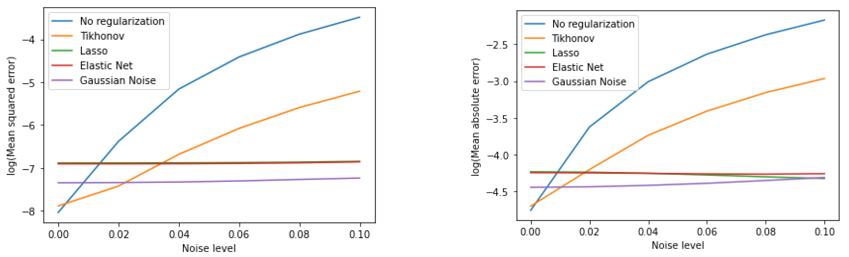
4.4. Comparison of the Different Methods

The Table 1 and Table 2, and Figure 6 shows the mean squared error and the mean absolute errors, which correspond to the errors calculated using 2 and 1 norms, respectively. The error is calculated as the difference between the actual and predicted conductivities on the entire test set for all the different methods where the Gaussian width is fixed. The vertical axis in Figure 6 is taken in the logarithmic scale for convenience due to the significant differences in the error for the different models. The previous section shows that the Lasso and Elastic Net had worse image reconstructions than the other methods. We find that the rbf network without regularization has the highest error and the Tikhonov regularization slightly improves the reconstructions. In our simulations, we find that the best approach is to add different levels of Gaussian noise to the data and train the RBF network on those data to build robustness to noise for the model.

5. Conclusions

We solve the Calderón inverse problem using an RBF network as demonstrated in the literature [21,22,23,24,25,26,35]. The previous approaches in the literature used various parameters for the radial basis function networks and different optimization methods without extensive regularization. We compared the performance of the networks for other choices of parameters, such as the width of the Gaussian activation function and three types of regularization. We also perform robustness studies for the proposed approach using an RBF network with regularization.
We conclude that using an rbf network with the same width for a Gaussian activation function provides the best results. Using different widths of the Gaussians may fit the data better. However, it increases the number of parameters for the network, making the parameter estimation problem harder. Even though it performs very well on the training set, it performs poorly on new examples outside of the training set. Using too many radial basis functions in the network also causes overfitting. However, by adding some regularization terms, we can mitigate the overfitting problem even for many RBFs in the hidden layer. The existence of a regularization term in the RBF loss function optimization problem is absent primarily in the treatment of the EIT inverse problem in the literature [21,22,23,24,25,26]. We demonstrate that regularization is necessary to obtain a proper inverse solver of EIT. The RBF network cannot reconstruct well outside the training data without regularization. Even though regularization causes the quality of the reconstructed image to deteriorate, it improves stability by correctly reconstructing images when tested on unseen data.
In summary, we conclude that by looking at the R 2 score, one can determine the optimal number of radial basis functions; the fixed-width radial basis function network with regularization results in improved performance. The fixed-width Gaussian with Tikhonov regularization performs very well. The regularization helps reconstruct the images outside of the training data. The regularization may cause the reconstruction quality to deteriorate. However, the stability is much improved. In terms of robustness, the RBF with Lasso and Elastic Net seem more robust compared to Tikhonov.

Author Contributions

Methodology, implementation, and writing of manuscript—C.A.F., P.S. and R.A.S.; supervision, review, and editing—T.K., P.S. and T.S. All authors have read and agreed to the published version of the manuscript.

Funding

This research received no external funding.

Data Availability Statement

The data that support the findings of this study are available from the corresponding author upon request.

Conflicts of Interest

The authors declare no competing conflict of interest.

References

  1. Cheney, M.; Isaacson, D.; Newell, J.C. Electrical impedance tomography. SIAM Rev. 1999, 41, 85–101. [Google Scholar] [CrossRef]
  2. Harris, N.; Suggett, A.; Barber, D.; Brown, B. Applications of applied potential tomography (APT) in respiratory medicine. Clin. Phys. Physiol. Meas. 1987, 8, 155. [Google Scholar] [CrossRef]
  3. Akbarzadeh, M.; Tompkins, W.; Webster, J. Multichannel impedance pneumography for apnea monitoring. In Proceedings of the Twelfth Annual International Conference of the IEEE Engineering in Medicine and Biology Society, Philadelphia, PA, USA, 1–4 November 1990; IEEE: Philadelphia, PA, USA, 1990; pp. 1048–1049. [Google Scholar]
  4. Colton, D.L.; Ewing, R.E.; Rundell, W. Inverse Problems in Partial Differential Equations; Siam: Philadelphia, PA, USA, 1990; Volume 42. [Google Scholar]
  5. Borcea, L. Electrical impedance tomography. Inverse Probl. 2002, 18, R99. [Google Scholar] [CrossRef]
  6. Ramirez, A.; Daily, W.; LaBrecque, D.; Owen, E.; Chesnut, D. Monitoring an underground steam injection process using electrical resistance tomography. Water Resour. Res. 1993, 29, 73–87. [Google Scholar] [CrossRef]
  7. Kaup, P.G.; Santosa, F.; Vogelius, M. Method for imaging corrosion damage in thin plates from electrostatic data. Inverse Probl. 1996, 12, 279. [Google Scholar] [CrossRef]
  8. Alessandrini, G.; Beretta, E.; Santosa, F.; Vessella, S. Stability in crack determination from electrostatic measurements at the boundary-a numerical investigation. Inverse Probl. 1995, 11, L17. [Google Scholar] [CrossRef]
  9. Alessandrini, G.; Rondi, L. Stable determination of a crack in a planar inhomogeneous conductor. SIAM J. Math. Anal. 1999, 30, 326–340. [Google Scholar] [CrossRef]
  10. Hyvonen, N.; Seppanen, A.; Staboulis, S. Optimizing electrode positions in electrical impedance tomography. SIAM J. Appl. Math. 2014, 74, 1831–1851. [Google Scholar] [CrossRef]
  11. Boyle, A.; Adler, A. The impact of electrode area, contact impedance and boundary shape on EIT images. Physiol. Meas. 2011, 32, 745. [Google Scholar] [CrossRef]
  12. Khalighi, M.; Vahdat, B.V.; Mortazavi, M.; Hy, W.; Soleimani, M. Practical design of low-cost instrumentation for industrial electrical impedance tomography (EIT). In Proceedings of the 2012 IEEE International Instrumentation and Measurement Technology Conference Proceedings, Graz, Austria, 13–16 May 2012; IEEE: Graz, Austria, 2012; pp. 1259–1263. [Google Scholar]
  13. Pidcock, M.; Kuzuoglu, M.; Leblebicioglu, K. Analytic and semi-analytic solutions in electrical impedance tomography: I. Two-dimensional problems. Physiol. Meas. 1995, 16, 77–90. [Google Scholar] [CrossRef]
  14. Pidcock, M.; Kuzuoglu, M.; Leblebicioglu, K. Analytic and semi-analytic solutions in electrical impedance tomography. II. Three-dimensional problems. Physiol. Meas. 1995, 16, 91. [Google Scholar] [CrossRef] [PubMed]
  15. Calderón, A. On an inverse boundary value problem, Seminar on Numerical Analysis and its Applications to Continuum Physics (Rio de Janerio). 1980. Available online: https://www.scielo.br/j/cam/a/fr8pXpGLSmDt8JyZyxvfwbv/?lang=en (accessed on 19 August 2023).
  16. Victor, I. Inverse Problems for Partial Differential Equations; Springer: Berlin/Heidelberg, Germany, 1997. [Google Scholar]
  17. Astala, K.L. Paivarinta Calderon’s inverse conductivity problem in the plane. Ann. Math. 2003, 163, 265. [Google Scholar] [CrossRef]
  18. Barceló, T.; Faraco, D.; Ruiz, A. Stability of Calderón inverse conductivity problem in the plane. J. Math. Pures Appl. 2006, 88, 522–556. [Google Scholar] [CrossRef]
  19. Zhang, G. Uniqueness in the Calderón problem with partial data for less smooth conductivities. Inverse Probl. 2012, 28, 105008. [Google Scholar] [CrossRef]
  20. Imanuvilov, O.; Uhlmann, G.; Yamamoto, M. The Calderón problem with partial data in two dimensions. J. Am. Math. Soc. 2010, 23, 655–691. [Google Scholar] [CrossRef]
  21. Wang, C.; Lang, J.; Wang, H.X. RBF neural network image reconstruction for electrical impedance tomography. In Proceedings of the 2004 International Conference on Machine Learning and Cybernetics (IEEE Cat. No. 04EX826), Shanghai, China, 26–29 August 2004; IEEE: Shanghai, China, 2004; Volume 4, pp. 2549–2552. [Google Scholar]
  22. Wang, P.; Li, H.l.; Xie, L.l.; Sun, Y.c. The implementation of FEM and RBF neural network in EIT. In Proceedings of the 2009 Second International Conference on Intelligent Networks and Intelligent Systems, Tianjin, China, 1–3 November 2009; IEEE: Tianjin, China, 2009; pp. 66–69. [Google Scholar]
  23. Hrabuska, R.; Prauzek, M.; Venclikova, M.; Konecny, J. Image reconstruction for electrical impedance tomography: Experimental comparison of radial basis neural network and Gauss–Newton method. IFAC-PapersOnLine 2018, 51, 438–443. [Google Scholar] [CrossRef]
  24. Wang, H.; Liu, K.; Wu, Y.; Wang, S.; Zhang, Z.; Li, F.; Yao, J. Image reconstruction for electrical impedance tomography using radial basis function neural network based on hybrid particle swarm optimization algorithm. IEEE Sens. J. 2020, 21, 1926–1934. [Google Scholar] [CrossRef]
  25. Michalikova, M.; Abed, R.; Prauzek, M.; Koziorek, J. Image reconstruction in electrical impedance tomography using neural network. In Proceedings of the 2014 Cairo International Biomedical Engineering Conference (CIBEC), Giza, Egypt, 11–13 December 2014; IEEE: Giza, Egypt, 2014; pp. 39–42. [Google Scholar]
  26. Michalikova, M.; Prauzek, M.; Koziorek, J. Impact of the radial basis function spread factor onto image reconstruction in electrical impedance tomography. IFAC-PapersOnLine 2015, 48, 230–233. [Google Scholar] [CrossRef]
  27. Griffiths, D.J. Introduction to Electrodynamics; AIP Publishing: New York, NY, USA, 2005. [Google Scholar]
  28. Jackson, J.D. Classical Electrodynamics; AIP Publishing: New York, NY, USA, 1999. [Google Scholar]
  29. Folland, G. Introduction to Partial Differential Equations; Mathematical Notes; Princeton University Press: Princeton, NJ, USA, 1995; Volume 17. [Google Scholar]
  30. Somersalo, E.; Cheney, M.; Isaacson, D. Existence and uniqueness for electrode models for electric current computed tomography. SIAM J. Appl. Math. 1992, 52, 1023–1040. [Google Scholar] [CrossRef]
  31. Kupis, S. Methods for the Electrical Impedance Tomography Inverse Problem: Deep Learning and Regularization with Wavelets. Ph.D. Thesis, Clemson University, Clemson, SC, USA, 2021. [Google Scholar]
  32. Vauhkonen, P. Image Reconstruction in Three-Dimensional Electrical Impedance Tomography (Kolmedimensionaalinen Kuvantaminen Impedanssitomografiassa); University of Kuopio: Kuopio, Finland, 2004. [Google Scholar]
  33. Park, J.; Sandberg, I.W. Universal approximation using radial-basis-function networks. Neural Comput. 1991, 3, 246–257. [Google Scholar] [CrossRef]
  34. Adler, A.; Lionheart, W.R. Uses and abuses of EIDORS: An extensible software base for EIT. Physiol. Meas. 2006, 27, S25. [Google Scholar] [CrossRef] [PubMed]
  35. Dimas, C.; Uzunoglu, N.; Sotiriadis, P. An efficient Point-Matching Method-of-Moments for 2D and 3D Electrical Impedance Tomography Using Radial Basis functions. IEEE Trans. Biomed. Eng. 2021, 69, 783–794. [Google Scholar] [CrossRef] [PubMed]
Figure 1. An rbf network. The hidden layer contains k radial basis functions { ϕ 1 . . ϕ k } and w i j are weights that need to be optimized. The input data set consists of n points { x 1 , , x n } and the rbf neural network gives an output data set of m points { y 1 , , y m } .
Algorithms 16 00461 g001
Figure 2. Mesh used for solving the forward problem.
Algorithms 16 00461 g002
Figure 3. Coefficient of determination R 2 vs. number of RBFs in hidden layer for different RBF network models. (a) RBF network with no regularization and variable Gaussian width. (b) RBF network with no regularization and fixed Gaussian width. (c) RBF network with Tikhonov regularization and variable Gaussian width. The regularization parameter λ is 10 5 . (d) RBF network with Tikhonov regularization and fixed Gaussian width. The regularization parameter λ is 10 5 .
Algorithms 16 00461 g003
Figure 4. Reconstruction images by all the different models. The true conductivity is shown in a finer mesh. The images were reconstructed on a coarser mesh. The models (except the Gaussian noise model) were trained on data with 4 % Gaussian noise, while the test data had 6 % Gaussian noise. (a) True conductivity distribution. (b) Reconstruction with fixed Gaussian width and no regularization. (c) Reconstruction with variable Gaussian width and no regularization. (d) Reconstruction with fixed Gaussian width and Tikhonov regularization. Regularization parameter λ = 10 5 . (e) Reconstruction with variable Gaussian width and Tikhonov regularization. Regularization parameter λ = 10 5 . (f) Reconstruction with fixed Gaussian width and Lasso regularization. Regularization parameter λ = 10 4 . (g) Reconstruction with variable Gaussian width and Lasso regularization. Regularization parameter λ = 10 4 . (h) Reconstruction with fixed Gaussian width and Elastic Net regularization. Regularization parameters in Equation (22) are λ 1 = 10 5 and λ 2 = 5 × 10 2 . (i) Reconstruction with variable Gaussian width and Elastic Net regularization. Regularization parameters in Equation (22) are λ 1 = 10 5 and λ 2 = 5 × 10 2 . (j) Reconstruction with fixed Gaussian width and the training data containing different levels of Gaussian noise. (k) Reconstruction with variable Gaussian width and the training data containing different levels of Gaussian noise.
Algorithms 16 00461 g004aAlgorithms 16 00461 g004b
Figure 5. Reconstructed images and the original conductivity distribution for a triple-inclusion example with 5 % Gaussian noise. All the models were trained on single- and double-inclusion examples only, and had fixed Gaussian width b j = 1 . (a) True conductivity distribution. (b) Reconstruction without regularization. (c) Reconstruction with Tikhonov regularization. Regularization parameter λ = 10 5 . (d) Reconstruction with Lasso regularization. Regularization parameter λ = 10 4 . (e) Reconstruction with Elastic Net regularization. Regularization parameters in Equation (22) are λ 1 = 10 5 and λ 2 = 5 × 10 2 . (f) Reconstruction with no regularization and where the training data contained different levels of Gaussian noise.
Algorithms 16 00461 g005
Figure 6. Comparison of the performance of the different methods with noise. The training set had no noise, except for the Gaussian noise method. All the models have fixed Gaussian width rbf in the hidden layer.
Algorithms 16 00461 g006
Table 1. Mean squared error ± standard deviation for the different methods.
NoiseNo RegularizationTikhonovLassoElastic NetGaussian Noise
0%0.0003 ± 0.00190.0004 ± 0.00230.001 ± 0.00530.001 ± 0.00510.0006 ± 0.0036
2%0.0017 ± 0.00460.0006 ± 0.00250.001 ± 0.00530.001 ± 0.00520.0006 ± 0.0036
4%0.0057 ± 0.01520.0012 ± 0.00350.001 ± 0.00530.001 ± 0.00520.0007 ± 0.0036
6%0.0121 ± 0.03230.0023 ± 0.00540.001 ± 0.00540.001 ± 0.00530.0007 ± 0.0037
8%0.0207 ± 0.05530.0037 ± 0.00840.001 ± 0.00550.001 ± 0.00540.0007 ± 0.0038
10%0.0307 ± 0.0820.0054 ± 0.01220.0011 ± 0.00560.001 ± 0.00550.0007 ± 0.0038
Table 2. Mean absolute error ± standard deviation for the different methods.
NoiseNo RegularizationTikhonovLassoElastic NetGaussian Noise
0%0.0085 ± 0.01580.009 ± 0.01710.0144 ± 0.02850.0143 ± 0.02820.0117 ± 0.0225
2%0.0266 ± 0.03140.0149 ± 0.01930.0144 ± 0.02850.0142 ± 0.02820.0118 ± 0.0225
4%0.0494 ± 0.05740.0238 ± 0.02610.0142 ± 0.02870.0141 ± 0.02830.012 ± 0.0226
6%0.0718 ± 0.08350.033 ± 0.03460.0138 ± 0.02890.014 ± 0.02850.0123 ± 0.0227
8%0.0935 ± 0.10910.0425 ± 0.04380.0135 ± 0.02930.014 ± 0.02880.0128 ± 0.023
10%0.1143 ± 0.13280.0516 ± 0.05280.0132 ± 0.02980.0141 ± 0.02910.0134 ± 0.0232
Disclaimer/Publisher’s Note: The statements, opinions and data contained in all publications are solely those of the individual author(s) and contributor(s) and not of MDPI and/or the editor(s). MDPI and/or the editor(s) disclaim responsibility for any injury to people or property resulting from any ideas, methods, instructions or products referred to in the content.

