Abstract
When designed correctly, radial basis function (RBF) neural networks can approximate mathematical functions to any arbitrary degree of precision. Multilayer perceptron (MLP) neural networks are also universal function approximators, but RBF neural networks can often be trained several orders of magnitude more quickly than an MLP network with an equivalent level of function approximation capability. The primary challenge with designing a high-quality RBF neural network is selecting the best values for the network’s “centers”, which can be thought of as geometric locations within the input space. Traditionally, the locations for the RBF nodes’ centers are chosen either through random sampling of the training data or by using k-means clustering. The current paper proposes a new algorithm for selecting the locations of the centers by relying on a structure known as an “opportunity matrix”. The performance of the proposed algorithm is compared against that of the random sampling and k-means clustering methods using a large set of experiments involving both a real-world dataset from the steel industry and a variety of mathematical and statistical functions. The results indicate that the proposed opportunity matrix algorithm is almost always much better at selecting locations for an RBF network’s centers than either of the two traditional techniques, yielding RBF neural networks with superior function approximation capabilities.
1. Introduction
Feed-forward, multilayer perceptron (MLP) neural networks have become highly valued and widely used tools in machine learning (ML) and artificial intelligence (AI) communities. One of the key reasons for this is that, given a sufficiently complex model, MLP neural networks have been shown to be universal function approximators, per Cybenko’s theorem [1]. This ability to approximate any function to any arbitrary degree of precision underlies the success of MLP-based neural networks in a very wide array of tasks, including binary, multilabel, and multiclass classification tasks, linear prediction tasks, speech and image recognition, and machine translation, among many others [2]. Unfortunately, high-precision function approximation using MLP neural networks often requires a large, complex model consisting of many nodes and many hidden layers, and this complexity can result in a lengthy and computationally expensive training process, particularly when it is necessary to evaluate the performance of many competing models [3,4].
1.1. Overview of RBF Neural Networks
Given the challenges that often arise when training MLP-based neural networks, AI/ML practitioners seeking a solution for high-precision function approximation may benefit greatly from considering another type of neural network architecture—that of a radial basis function (RBF) network [5]. In contrast with conventional MLP networks, RBF neural networks differ in that they rely on a single hidden layer of nodes in which nonlinear radial basis functions are used as the nodes’ activation functions. This particular type of neural network architecture has shown itself to be of value in a wide variety of practical applications, including solving partial differential equations [6], real-time facial recognition [7], computer vision [8], and signal processing [9], among many others.
Although RBF neural networks most commonly rely on Gaussian radial basis functions, other types of radial basis functions may be substituted when appropriate [10]. The standard Gaussian radial basis function is defined in Equation (1) below [11]. The parameter r in Equation (1) denotes the distance between an input value and the RBF node’s “center” (which will be discussed shortly), while the parameter σ controls the shape of the Gaussian. Euclidean distance is ordinarily used for r; however, the Mahalanobis distance measure may yield superior results in certain problem domains, such as pattern recognition [12].
After each input value passes through the RBF layer, the weighted outputs from the RBF nodes are linearly combined to yield the RBF network’s overall output [13]. An illustrative example of the standard RBF neural network architecture is provided in Figure 1. Importantly, it is only the weights between the RBF layer and the output layer (denoted in Figure 1) that need to be learned during the network training process.
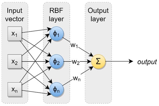
Figure 1.
Standard RBF neural network architecture.
Each RBF node in an RBF neural network is characterized by a “center” and a “width”. Each RBF node center takes the form of a vector of the same dimensionality as the input vector and can be conveniently conceptualized as a geometric location within the input space. For a Gaussian RBF node, the width is parameterized as the standard deviation, the value of which controls the rate at which the node’s influence diminishes as input values become more and more distant from the node’s center. During training, only those few RBF nodes whose centers are closest to an input value will experience any sort of significant activation, the effect of which is that only a small number of weights will be updated in response to the input value. Once the locations of the RBF centers have been chosen, finding optimal weights for an RBF network can be accomplished either through direct calculation by using a pseudoinverse approach [5,14] or via gradient descent [10,15]. Notably, the training process for RBF neural networks is often several orders of magnitude faster than for MLP-based neural networks with corresponding degrees of function approximation capability [5,16,17].
1.2. Selecting Widths and Centers for RBF Nodes
Although it is feasible to assign individual width values to each of the RBF nodes in an RBF neural network, doing so is typically unnecessary. Indeed, research has shown that Gaussian RBF networks using the same width value (i.e., the same standard deviation) for every RBF node retain their universal function approximation capability [18]. Equation (2) below defines a simple method for identifying the global width value σ to use for all of the RBF nodes in an RBF network [10]. The parameter in Equation (2) represents the maximum (typically Euclidean) distance between any two RBF node centers, while k denotes the total number of RBF nodes in the neural network.
While calculating the global width value to use in an RBF neural network is trivial, choosing the most suitable locations for the RBF nodes’ centers is much less straightforward. As noted previously, RBF neural networks are, in theory, universal function approximators; however, in practice, the ability of an RBF network to accurately approximate a function depends critically on the locations that have been chosen for the centers of its RBF nodes [10,19]. The reason for this is that the influence of each RBF node is localized to a specific region within the input space, with the extent of the region of influence depending on the value of the node’s width parameter [18]. A given RBF node’s influence on the network’s output will be quite strong when the distance between an input vector and the node’s center is small, but the extent of the node’s influence on the output will diminish rapidly as the distance between the node’s center and the input vector increases (vide supra, Equation (1)). Well-chosen centers will therefore allow the RBF network to more accurately approximate a target function than if the locations of the centers had been chosen poorly. This concept is illustrated for a target function with a single input value in Figure 2 below. The width of each Gaussian curve in Figure 2 indicates the region of the input space over which the corresponding RBF node exerts influence, while the size of each RBF node center represents the magnitude of the corresponding node’s weight in the RBF network (denoted in Figure 1).
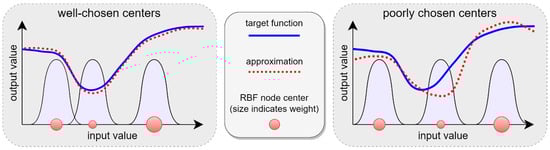
Figure 2.
The effect of RBF node center locations on function approximation accuracy.
As shown in Figure 2, the location of the RBF nodes’ centers plays a very important role in the overall performance of the RBF neural network [19]. For this reason, the overall task of training an RBF neural network is typically subdivided into two distinct phases, with the first phase involving the selection of the RBF nodes’ centers and widths, and the second phase involving the adjustment of the network’s weights with a view to minimizing error [10].
By a wide margin, the two most common strategies for choosing the locations of an RBF network’s centers are random sampling and k-means clustering [10,13]. Random sampling is the simplest and fastest of these two common strategies. Using this approach, a subset of k input values is randomly chosen from the available training data, with these k input values then being used directly as the locations for the RBF network’s centers. This approach is rational from the perspective of probability theory, since a sufficiently large random sample will approximate the distribution of the underlying population reasonably well [20]. As such, the resulting RBF nodes are likelier to be located near the regions of the input space that have the highest probability density than if the centers had been positioned equidistantly from one another within the input space.
The rationale underlying the k-means clustering strategy is similar to that of the random sampling strategy; i.e., to locate the RBF centers in areas of the input space that best represent the distribution of the underlying training data. Using the k-means approach, the training data (or a sample thereof) are run through the k-means vector quantization algorithm in order to group the input cases into k clusters. The centroids of the resulting k clusters are then used as the locations for the RBF nodes’ centers. Since the purpose of clustering is to partition the input data into distinct groups of similar cases [21], the k-means approach results in a solution in which each RBF center represents one distinct group of similarly located cases within the input data, and for which the corresponding RBF node will activate most strongly in the presence of an input value that is a member of its own group. These properties and the relative ease of implementation have made the k-means approach very popular among AI/ML practitioners when working with RBF neural networks [22].
1.3. Research Goal
The preceding discussion introduced RBF neural networks and their benefits, explained the role of RBF centers in the overall performance of an RBF neural network, and described the two most widely used methods of selecting the locations for an RBF network’s centers. With this foundational information in mind, we are now well equipped to understand the primary goal of the current research project.
In brief, the current paper seeks to develop a new algorithm—based on the concept of an “opportunity matrix”—whose purpose is to select locations for an RBF network’s centers that will consistently yield superior overall function approximation performance for the RBF neural network. In pursuit of this goal, the following section first describes the proposed opportunity matrix algorithm for selecting RBF node centers, and then provides details about the series of experiments that were conducted in order to compare the performance of the proposed algorithm against that of the standard random sampling and k-means clustering techniques. The results of the experiments are subsequently presented and discussed in Section 3. The paper concludes in Section 4 with a summary, a description of the study’s limitations, and suggestions for future research opportunities in this area. A graphical overview of the current study is provided in Figure 3 below.
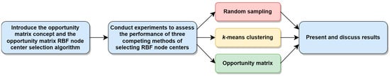
Figure 3.
Overview of the current study.
2. Materials and Methods
This section begins by introducing the concept of an opportunity matrix, and then proceeds with a detailed description of the proposed opportunity matrix algorithm for selecting the locations of RBF node centers in a radial basis function neural network. Following these preliminaries, this section next describes the series of experiments that were conducted in order to compare the performance of the proposed algorithm against that of the standard random sampling and k-means clustering approaches to selecting RBF node centers. For purposes of investigating the generalizability of the proposed algorithm, these experiments involve both a real-world dataset from the steel industry and the approximation of a variety of mathematical and statistical functions using a variety of RBF neural network models, each of which relies on a different number of RBF nodes. The results of the experiments—which reveal the overwhelming superiority of the proposed opportunity matrix algorithm—are then presented and discussed in Section 3.
2.1. The Opportunity Matrix
The core concept underlying the proposed algorithm is that of an “opportunity matrix”. In brief, an opportunity matrix is a fixed-size, d-dimensional container whose dimensionality matches that of the number of input features in the RBF network’s training data. If each training case contains a single input feature, the opportunity matrix will be a vector. Similarly, if each training case consists of two input features, the opportunity matrix will be two-dimensional, and so on. Each dimension in the opportunity matrix is mapped to one of the input features in the training data, with the number of items in each dimension being determined by partitioning the range of values in the dimension’s associated input feature into equidistantly spaced intervals. Alternatively, a quantile-based split rather than an equidistant split may be used if the AI/ML practitioner prefers to take the distributional properties of the data into account. Note that these methods of partitioning can be implemented for both continuous and discrete input features, and can be readily adapted for use with categorical features. As an illustrative example, imagine a scenario in which an AI/ML practitioner wishes to develop an RBF neural network. The available training data contain two continuous input features, a and b, with the range of feature a being and the range of feature b being . Further, assume that the AI/ML practitioner wishes to partition both of the input features into five equidistantly spaced intervals, such that and . In this scenario, the resulting opportunity matrix would be structured as shown in Figure 4 below.
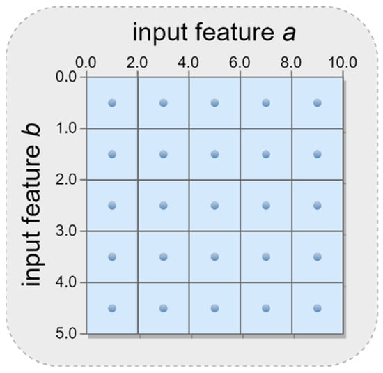
Figure 4.
Example of an opportunity matrix structure for an RBF network with two input features.
In the scenario illustrated above, the opportunity matrix contains unique elements, each of which represents a bounded region of the overall input space. The first foundational idea of the opportunity matrix approach is that the centroid of each of these bounded regions (which are signified by dots in Figure 3) represents a potential opportunity for the location of an RBF node in a radial basis function neural network. It naturally follows that the quantity defines the upper limit for the number of RBF nodes that could feasibly appear in the network. An AI/ML practitioner must therefore be judicious when choosing the number of intervals into which each input feature should be partitioned. Note also that this framework can be easily extended into higher-dimensional spaces to accommodate any possible number of input features.
The second foundational idea of the opportunity matrix approach is that the RBF network is constructed incrementally by adding one RBF node at a time. To accomplish this, the AI/ML practitioner begins by first selecting a reasonably sized random sample of the training data. An initial RBF node is then added to the neural network structure, with the location of the initial node’s center being chosen either randomly or by relying on the centroid of all of the sample’s input features. The single weight for this simplest of all possible RBF neural networks is then learned using the sample of the training data. When training is complete, each element in the opportunity matrix is populated with the average prediction error for all of the input values that lie within the element’s boundaries. The opportunity matrix is then examined to identify the element with the largest average error that does not already have an associated RBF node, and that element’s centroid is then used as the location for the next RBF node that is added to the neural network. The opportunity matrix is then emptied and the process is repeated, with one new RBF node being added during each iteration until a chosen stopping criterion has been met. An illustrative example of an opportunity matrix being used to iteratively identify the locations of new RBF nodes is provided in Figure 5. The number appearing inside each element of the opportunity matrix in Figure 5 indicates the mean prediction error for input values that fall within the element’s boundaries during the corresponding iteration.
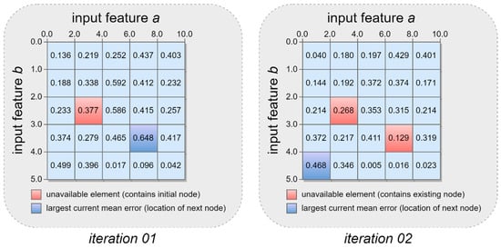
Figure 5.
Example of an opportunity matrix being used to iteratively select RBF node centers.
Recall from the previous discussion that the potential influence of each RBF node on the neural network’s output is maximal at the node’s center and that this influence diminishes as input values grow more and more distant from the node’s center. With this in mind, one can readily understand how iteratively locating new RBF nodes in regions of the input space where the mean prediction error is currently highest can yield substantial improvements in the RBF neural network’s overall performance. This tendency is illustrated in the transition from iteration 01 to iteration 02 in Figure 5 above.
2.2. The Opportunity Matrix RBF Center Selection Algorithm
Having related the foundational concepts underlying the opportunity matrix and its use, we are now properly equipped to proceed with a complete description of the opportunity matrix RBF center selection algorithm. In what follows, the steps in the Algorithm 1 are described textually rather than symbolically in order to ensure clarity, as well as to allow for additional commentary.
| Algorithm 1: Using an opportunity matrix to select centers for an RBF neural network. |
|
The proposed opportunity matrix algorithm is summarized graphically in Figure 6 below.
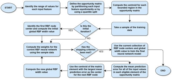
Figure 6.
Using an opportunity matrix to select centers for an RBF neural network.
2.3. Evaluative Experiments
Having presented the proposed opportunity matrix algorithm for selecting RBF node centers, it is now possible to describe the series of experiments that were conducted in order to compare the performance of the opportunity matrix approach against that of the standard random sampling and k-means clustering techniques. In total, 25 experiments were conducted in order to evaluate the performance characteristics of the competing RBF node selection methods under a variety of different conditions. The first 20 of these experiments involved the task of using RBF neural networks to approximate four different functions, two of which were mathematical optimization functions (Himmelblau’s function [24] and the Hosaki function [25]) and two of which were statistical functions (the Poisson distribution probability mass function [26] and the t-distribution cumulative distribution function [27]). These specific functions were chosen because of their common use in optimization research and statistics, as well as to enhance the generalizability of the experiments by including functions from different domains that involve both continuous and discrete parameters. Visualizations of these four functions are provided in Figure 7, Figure 8, Figure 9 and Figure 10 below. The color spectrum in these figures ranges from blue to red, signaling comparatively small to large output values, respectively. For the remaining five experiments, the performance of the proposed opportunity matrix algorithm was compared with that of the standard random sampling and k-means clustering techniques using a real-world energy consumption dataset from the steel industry [28]. This dataset, which is publicly available from the UC Irvine Machine Learning Repository [29], contains several continuous and categorical features that were used to predict the electrical power consumption of a steel manufacturing facility.
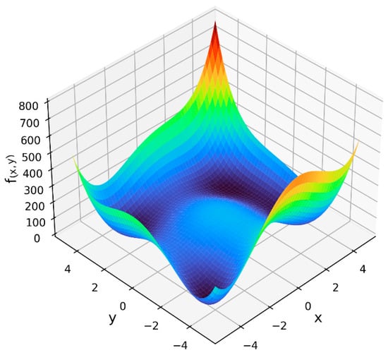
Figure 7.
Himmelblau’s function.
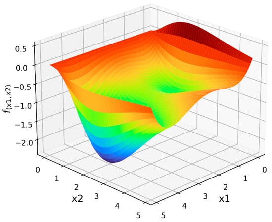
Figure 8.
Hosaki function.
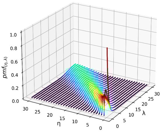
Figure 9.
Poisson distribution probability mass function.
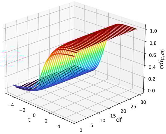
Figure 10.
t-Distribution cumulative distribution function.
Formally, the four functions depicted above are defined as shown in Equations (3)–(6) below. In the experiments, values for Himmelblau’s function and the Hosaki function were computed directly, while values for the Poisson distribution probability mass function and the t-distribution cumulative distribution function were computed using the Python SciPy library [30].
Himmelblau’s function:
Hosaki function:
Poisson distribution probability mass function (PMF):
where is the number of occurrences and is the expected value.
t-Distribution cumulative distribution function (CDF):
where is the observed t-value, is the degrees of freedom, is the regularized incomplete beta function [31], and .
In addition to the steel industry power consumption dataset, the functions defined in Equations (3)–(6), and the three different RBF node selection methods, five possible values for the number of RBF nodes () were used in the experiments, with . Each experimental condition thus involved (1) using three RBF networks, each of which sought to approximate one of the four functions defined above or predict the power consumption of a steel manufacturing facility; (2) using one of the possible values of for the number of RBF nodes in those networks; and (3) using the three competing RBF node selection methods to choose the locations of the RBF node centers, with one of the different methods (random sampling, k-means clustering, or the proposed opportunity matrix algorithm) being used for each of the experiment’s three RBF networks. Given the five different function approximation tasks and the five possible values for the number of RBF nodes, a total of experiments were carried out in the study, each of which compared the performances of the three competing RBF node selection methods. Each experiment was also repeated 30 times in order to ensure that the distributions of the resulting performance metrics would be approximately Gaussian, per the central limit theorem [32].
In each experiment, the same data were used to train all three competing RBF neural networks. Each of these neural networks also had precisely the same structure (including the number of RBF nodes) and relied on the same Adam stochastic optimization algorithm for learning the network’s weights [33]. The only difference among the competing neural networks was therefore the locations of their RBF node centers, which, as noted above, were chosen by a different RBF node selection method for each network. In this way, any statistically significant differences in the function approximation performance among the three competing neural networks could be attributed solely to the method that was used to select the networks’ RBF node centers.
With specific respect to the data, the real-world steel industry dataset contained 35,040 cases, while 1,000,000 cases were used in each experimental trial involving one of the four mathematical optimization and statistical functions. With respect to the latter, the data were generated randomly within the experimental boundaries of each function’s input parameters. Either a uniform continuous or uniform discrete sampling distribution was used when randomly generating these data, depending on the nature of each input parameter. After computing the input parameters’ associated output values for each mathematical or statistical function, each dataset was then randomly split into training and testing sets, with the training set consisting of 80% of the cases and the testing set containing the remaining 20% of the cases. For the experiments involving Himmelblau’s function, the and input parameters were both bounded by the interval , while for the experiments involving the Hosaki function, the and input parameters were both bounded by the interval . For the experiments involving the Poisson distribution probability mass function, the parameter used values in the set , while the parameter was bounded by the interval . Finally, for the experiments involving the t-distribution cumulative distribution function, values for the parameter were bounded by the interval , while the parameter was constrained to values in the set . All of these experimental boundaries are included in the depictions of the four test functions provided in Figure 7, Figure 8, Figure 9 and Figure 10.
Since using the opportunity matrix algorithm to obtain the locations of RBF node centers requires an AI/ML practitioner to make several choices, it is necessary and appropriate to provide specific details about how the algorithm was used in the current study in order to ensure that the study’s results can be reproduced. To begin, Step #2 of Algorithm 1 requires a decision about the number of intervals into which the range of values for each input parameter should be partitioned. In the current study, the range of values for all of the mathematical and statistical functions’ continuous input features was subdivided into 100 equidistantly spaced intervals, while for discrete input features, each unique item in the sets defined immediately above was used as the basis for its own partition in the feature’s corresponding dimension of the opportunity matrix. For the real-world steel industry dataset, each of the continuous input features was partitioned using a quartile split, with the values for each discrete input feature again being used as the basis for its own partition in the opportunity matrix.
Step #4 in Algorithm 1 requires a reasonably sized sample of the overall training data. For the experiments involving the mathematical and statistical functions, 5% (or 40,000) of the available cases were randomly sampled from the overall training data for use in the opportunity matrix algorithm, while a random sample of 10,000 cases was used for the experiments involving the steel industry power consumption dataset. For Step #7 in Algorithm 1, the value of that was being considered in the current experimental trial was used as the stopping criterion, thus ensuring that a sufficient number of RBF node centers would be available to support the needs of the current trial. Finally, the RBF networks used in the opportunity matrix algorithm were trained using the Adam stochastic optimizer [33] with a batch size of 128 cases across 256 training epochs.
As noted previously, the overall goal of the experiments was to compare the RBF node selection performance of the proposed opportunity matrix algorithm against that of the standard random sampling and k-means clustering methods under a wide variety of different conditions. Each of these conditions was evaluated in a distinct experiment involving 30 consecutive trials. For each trial, three RBF neural networks were used that relied on the same data, structure, and training algorithm, with the only difference among the networks being the method that was used to select the locations of their RBF node centers. Each final neural network in the trials was trained using a batch size of 128 training cases across 1024 epochs, after which training was considered complete. The experiments themselves were run sequentially using a fixed hardware configuration on the Google Colaboratory platform [34].
When the three RBF neural networks that were considered in each experimental trial had been fully trained, their performance was assessed by measuring the mean absolute error (MAE) of the networks’ associated predictions on the data in the testing set. As with the training data, exactly the same testing data were used to evaluate all of the neural networks in each trial. With 30 trials per experiment, every experiment resulted in 30 MAE values for each of the three competing methods of selecting RBF node centers that corresponded to the experiment’s unique combination of test function and number of RBF nodes within the study’s overall experimental framework. Finally, the MAE values obtained from the opportunity matrix algorithm, the random sampling method, and the k-means clustering method were statistically compared against each other using Welch’s t-tests [35]. Unlike most other t-tests, Welch’s t-tests allow for the comparison of independent samples that have unequal variances. Since there was no ex ante reason to expect the distributional variances of the performance metrics obtained from each competing RBF center selection method to be equal, Welch’s t-tests provided an appropriate statistical foundation for comparing the experimental results.
3. Results and Discussion
As described in the previous section, the experiments carried out in this study were designed to compare the performance of the proposed opportunity matrix algorithm against that of the standard random sampling and k-means clustering methods of selecting RBF node centers under a variety of different conditions. Each of these experimental conditions involved assessing the function approximation performance of an RBF neural network with 16, 32, 64, 128, or 256 RBF nodes using either the real-world steel industry dataset or one of the four functions described in Section 2.3, with each experiment being repeated across 30 trials. The results obtained from the experiments for each of the five function approximation tasks are presented in Table 1, Table 2, Table 3, Table 4 and Table 5 below.

Table 1.
Experimental results for the approximation of Himmelblau’s function.
Table 2.
Experimental results for the approximation of the Hosaki function.
Table 3.
Experimental results for the approximation of the Poisson distribution PMF.
Table 4.
Experimental results for the approximation of the t-distribution CDF.
Table 5.
Experimental results for the real-world steel industry energy consumption dataset.
When considering Table 1, Table 2, Table 3, Table 4 and Table 5 above, it is clear that the average mean absolute error of the RBF neural networks’ predictions tends to decrease as the number of RBF nodes increases, regardless of the function being approximated or the method that was used to select the locations of the nodes’ centers. This behavior is consistent with both theory and past research into RBF neural networks [10,18], and serves to strengthen the face validity of the study’s experimental framework. As noted in Section 1, RBF neural networks are capable of approximating any continuous function to any arbitrary degree of precision, and it is evident that this function approximation capability depends in part on the number of RBF nodes that are included in the network architecture. What is also evident from the average MAEs reported in Table 1, Table 2, Table 3, Table 4 and Table 5 above is that the ability of an RBF neural network to accurately approximate a function depends critically on the locations of the network’s RBF node centers. Put simply, an RBF neural network with well-chosen centers will deliver more accurate predictions than an otherwise identical RBF neural network with poorly chosen centers. With this in mind, the primary goal of the current research was to propose a new algorithm for selecting RBF centers based on the concept of an opportunity matrix, and then experimentally investigate the proposed algorithm’s performance in comparison with the two most widely used methods of selecting centers.
Generally speaking, Welch’s t-test results reported in Table 1, Table 2, Table 3, Table 4 and Table 5 reveal that the proposed opportunity matrix algorithm is typically able to statistically outperform the standard random sampling and k-means clustering methods of selecting centers for RBF neural networks, often by a very large margin. Indeed, among the 25 head-to-head comparisons with the random sampling method, the performance of the opportunity matrix algorithm was statistically superior in 24 of the experimental conditions and was statistically indistinguishable in the remaining condition. Among the 25 head-to-head comparisons with the k-means clustering method, the performance of the opportunity matrix algorithm was statistically superior in 21 of the experimental conditions, statistically indistinguishable in 3 experimental conditions, and statistically inferior in just 1 of the 25 conditions. Collectively, then, the proposed opportunity matrix algorithm was able to select RBF node centers that resulted in statistically better-performing RBF neural networks in 90% of the head-to-head comparisons with alternative methods that were considered in the experiments. Among the remaining head-to-head comparisons, the performance of the proposed opportunity matrix algorithm was statistically identical to an alternative method in 8% of the cases and was statistically inferior in only 2% of the cases. The results of the experiments, therefore, indicate that the proposed opportunity matrix algorithm is generally superior to the standard random sampling and k-means clustering methods in terms of its ability to select high-quality locations for RBF node centers. As shown in the experiments, these superior center locations directly result in better-performing RBF neural networks.
Given the observed superiority of the proposed opportunity matrix algorithm, it may be instructive to consider the locations of the RBF node centers that were chosen by the algorithm in comparison with the standard random sampling and k-means techniques. Figure 11 below, therefore, provides an illustrative example of the RBF center locations that were chosen by the opportunity matrix, random sampling, and k-means clustering techniques for a neural network with 64 RBF nodes that was seeking to approximate Himmelblau’s function.
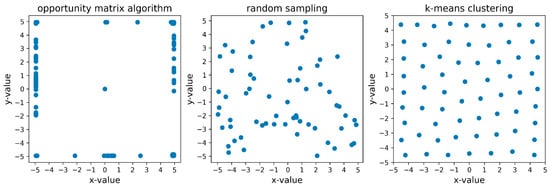
Figure 11.
Comparison of RBF node center locations chosen by the opportunity matrix, random sampling, and k-means clustering techniques for a neural network seeking to approximate Himmelblau’s function using 64 RBF nodes.
As shown in Figure 11 above, excepting for one centrally located RBF node center, all of the other RBF centers chosen by the opportunity matrix algorithm were peripherally located when attempting to approximate Himmelblau’s function. By contrast, the RBF center locations chosen by the k-means clustering technique were approximately equidistantly distributed throughout the bounded region of the input space, while no obvious distributional pattern was present for the RBF center locations chosen by the random sampling technique. Recalling from Section 2 that the values for the input parameters in the experiments involving Himmelblau’s function were randomly generated from a uniform distribution, the theoretical rationale underlying the use of random sampling and k-means clustering is evident in Figure 11; i.e., to locate the RBF node centers in areas of the input space that best represent the distribution of the input features in the training data.
Rather than focusing exclusively on the distribution of the inputs, the theoretical rationale underlying the opportunity matrix technique is to locate the RBF node centers in areas of the input space that are, on average, the largest sources of prediction error. When considering the RBF center locations chosen by the opportunity matrix algorithm in Figure 11 in conjunction with the visualization of Himmelblau’s function provided in Figure 7, it becomes immediately clear why the opportunity matrix algorithm chose the RBF center locations that it did—to target the areas of the input space that otherwise would likely yield large prediction errors. These visual elements are reproduced and presented side by side as Figure 12 below for the convenience of the reader. The core insight to be learned from this discussion—and the reason for the opportunity matrix algorithm’s superior performance—is that identifying and taking steps to mitigate the most significant sources of prediction error appears to be a very effective strategy for selecting the locations of the centers in an RBF neural network.
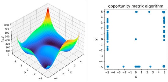
Figure 12.
Himmelblau’s function and the corresponding RBF center locations that were chosen by the opportunity matrix algorithm.
Finally, some consideration of the computational resources and wall-clock time required by each competing method of selecting RBF node center locations is merited. Assuming that the available training cases have been randomly shuffled, then the random sampling technique can reasonably be expected to require minimal memory and wall-clock time, since one may simply use the input values for the first k cases in the training data as the center locations for a network with k RBF nodes. By contrast, the k-means clustering technique can be expected to require much more memory and wall-clock time than random sampling, since the k-means clustering algorithm is known to be NP-hard [36] and requires the repeated calculation of the distance between each of the k centroids and every available case in the training data. The proposed opportunity matrix algorithm can, of course, be expected to require substantially more wall-clock time than either of the random sampling or k-means clustering methods, since it relies on an iterative approach in which one RBF node is identified per iteration, with the additional requirement that the weights of an RBF neural network be learned during each of those iterations.
The expectations related above notwithstanding, a direct evaluation of the memory and wall-clock time required by each method of selecting RBF center locations was undertaken in order to provide a measure of empirical insight into this issue, with the approximation of the Hosaki function serving as the basis of the evaluation. To ensure equitable comparisons, the memory and wall-clock time requirements for all three RBF node selection methods were measured using a single thread on a single CPU. When conducting the comparisons, the sample size and RBF neural network training parameters that were used to select the RBF center locations with the opportunity matrix technique matched those described previously in Section 2. The results of these measurements are provided in Table 6 below. Note that the peak memory requirements shown in the table include overhead items that were needed to run the Google Colaboratory environment, such as external libraries and the memory profiler itself. Nevertheless, these values provide insights into the comparative memory demands of the three different methods of selecting RBF center locations.
Table 6.
Average peak memory and wall-clock time required to select RBF node centers for the Hosaki function.
As shown in Table 6 above, the random sampling method required both the least memory and the least wall-clock time to select RBF node centers for the Hosaki function. Although the wall-clock time required by the k-means clustering method fell between the time required by the random sampling and opportunity matrix methods, the k-means clustering method consistently required the largest amount of memory to complete the RBF center selection task. As expected, the opportunity matrix algorithm required much more wall-clock time than either of the other two competing methods, with its memory requirements falling between those of the random sampling and k-means clustering methods. It is important to note, however, that the measurements reported in Table 6 were obtained using a single thread on a single CPU. Since the opportunity matrix algorithm involves the iterative training of a series of RBF neural networks, one might reasonably expect that substantially less wall-clock time would be required by the opportunity matrix method if a hardware accelerator, such as a GPU or a tensor processing unit, were used to facilitate the RBF node selection process.
4. Summary, Limitations, and Concluding Remarks
4.1. Summary of Contributions and Findings
This paper proposed a new algorithm based on the concept of an opportunity matrix for selecting the locations of the centers in a radial basis function (RBF) neural network. The opportunity matrix approach involves first partitioning the input space into several regions, and then iteratively adding one RBF node at a time to the structure of the neural network. In each iteration, a small sample of the available training data is used as the basis for estimating the weights for the current RBF neural network architecture. These weights are subsequently utilized to generate predictions for the sample inputs, with the corresponding prediction errors being recorded in the appropriate regions of the opportunity matrix. Finally, the opportunity matrix is examined to identify the region of the input space that currently exhibits the largest average error, and the centroid of that region is used as the center for the next RBF node that is added to the neural network structure. New RBF nodes are iteratively added to the neural network in this manner until a stopping criterion is met.
A large set of experiments was conducted in order to evaluate the performance of the proposed opportunity matrix algorithm in comparison with the two most widely used methods of selecting centers for RBF neural networks, namely, random sampling of the training data and k-means clustering. The experiments involved the task of using RBF neural networks to approximate four different well-known mathematical optimization and statistical functions or to predict the energy consumption for a steel manufacturing facility. To ensure generalizability, two of these functions used only continuous input parameters, while the remaining two functions and the real-world steel industry dataset included both continuous and discrete input parameters. A variety of neural network architectures were also considered in the experiments, with each network containing 16, 32, 64, 128, or 256 RBF nodes. The results of the experiments revealed the general superiority of the proposed opportunity matrix algorithm. Specifically, in head-to-head comparisons with the standard random sampling and k-means clustering techniques, RBF neural networks whose center locations were chosen using the opportunity matrix approach were found to generate statistically superior predictions 90% of the time. Among the remaining experimental conditions, the opportunity matrix algorithm yielded statistically identical outcomes in 8% of the cases, and was found to perform more poorly than one of the standard methods in only 2% of the cases. It can therefore be concluded that using the proposed opportunity matrix algorithm to select the locations of RBF node centers will, on average, result in RBF neural networks with superior function approximation capabilities.
4.2. Limitations and Opportunities for Future Research
Although careful and systematic efforts were taken in this study to investigate the performance of the proposed opportunity matrix algorithm in comparison with that of the standard random sampling and k-means clustering methods, there nevertheless remain several limitations to this work that require acknowledgement. First, the experiments described herein relied on one real-world dataset and four different mathematical optimization and statistical functions. Care was taken to select well-known functions and a publicly available dataset that relied on both continuous and discrete input parameters, but any number of other functions or real-world datasets could have been used instead of the those that were considered in the study. Future work in this area should therefore endeavor to assess the performance of the opportunity matrix algorithm with other real-world datasets and other mathematical or statistical functions.
In addition to relying on just four different functions and one real-world dataset, the findings of the experiments reported herein are also limited insofar as each of the five testing scenarios considered in the study used a relatively small number of input parameters and involved just one output value each. While the opportunity matrix framework allows for any positive number of input parameters, and while there is no theoretical or mathematical reason to expect that the opportunity matrix algorithm would perform differently with functions that require a large number of input parameters or that have more than one output value, these conditions have not yet been assessed experimentally. Future work in this area should therefore endeavor to assess the performance of the opportunity matrix algorithm when using functions that require a wider variety of inputs and outputs.
Next, the opportunity matrix algorithm includes several tunable parameters whose values must be chosen by the AI/ML practitioner. Examples of these parameters include the number of intervals into which the range of values for each input parameter is partitioned, the size of the sample data that are used to iteratively identify RBF node center locations, and the stopping criterion that is used to terminate the algorithm. These tunable parameters are suitable targets for hyperparameter optimization, and future work in this area may be able to identify appropriate optimization techniques that can further improve the performance of the opportunity matrix algorithm.
Finally, the opportunity matrix algorithm requires substantially more wall-clock time than the random sampling or k-means clustering methods in order to choose the locations for an equivalent number of RBF nodes. It is reasonable to expect that this notable differential in wall-clock time could be reduced through the use of a hardware accelerator when running the opportunity matrix algorithm; however, this expectation has not yet been assed experimentally. AI/ML practitioners may take some comfort in knowing that the opportunity matrix algorithm will almost always yield a better-performing RBF neural network, but are nevertheless advised to consider the comparatively large amount of wall-clock time required by the opportunity matrix approach before deciding to apply it to their particular use case.
4.3. Concluding Remarks
This paper clearly demonstrated that the locations chosen for the RBF node centers in a radial basis function network are critically important to the network’s ability to generate accurate predictions. While it is true that an AI/ML practitioner can increase the accuracy of an RBF neural network by simply and lazily adding more RBF nodes to the network architecture, this is, I think, an incorrect approach. Indeed, the law of parsimony, as elegantly expressed in Occam’s razor, should serve as a guiding principle in the design of RBF neural network architectures. Excessively complex network structures require more time to train, make predictions more slowly, and unnecessarily consume finite computational resources. Why should a neural network with 100 RBF nodes be used when a network containing just 10 nodes with well-chosen RBF centers can generate equally accurate outputs? Radial basis function neural networks have many desirable properties—including fast learning, simple architecture, and the ability to accurately approximate nonlinear functions—that may allow them to play a key role in the modular development of artificial general intelligence [37]. To reach the scale of complexity and capability of the human brain, however, will require careful stewardship of computational resources. Approaches such as the opportunity matrix algorithm described herein have great potential to aid in these efforts by ensuring that each individual RBF neural network is as compact and efficient as possible.
Funding
This research received no external funding.
Data Availability Statement
The data obtained from the experiments may accessed at: https://drive.google.com/file/d/1_XzvaYKoIXDWgXYop-emK8UlfWYEe7IV/view?usp=sharing (accessed on 19 September 2023).
Conflicts of Interest
The author declares no conflict of interest.
References
- Cybenko, G. Approximation by Superpositions of a Sigmoidal Function. Math. Control Signals Syst. 1989, 2, 303–314. [Google Scholar] [CrossRef]
- Anderson, J.A. An Introduction To Neural Networks; MIT Press: Cambridge, MA, USA, 1998. [Google Scholar]
- Soper, D.S. Hyperparameter Optimization using Successive Halving with Greedy Cross Validation. Algorithms 2022, 16, 17. [Google Scholar] [CrossRef]
- Soper, D.S. Greed is Good: Rapid Hyperparameter Optimization and Model Selection using Greedy k-Fold Cross Validation. Electronics 2021, 10, 1973. [Google Scholar] [CrossRef]
- Broomhead, D.; Lowe, D. Multivariable Functional Interpolation and Adaptive Networks. Complex Syst. 1988, 2, 321–355. [Google Scholar]
- Lagaris, I.E.; Likas, A.C.; Papageorgiou, D.G. Neural-Network Methods for Boundary Value Problems with Irregular Boundaries. IEEE Trans. Neural Netw. 2000, 11, 1041–1049. [Google Scholar] [CrossRef]
- Yang, F.; Paindavoine, M. Implementation of an RBF Neural Network on Embedded Systems: Real-Time Face Tracking and Identity Verification. IEEE Trans. Neural Netw. 2003, 14, 1162–1175. [Google Scholar] [CrossRef]
- Cho, S.-Y.; Chow, T.W. Neural Computation Approach for Developing a 3D Shape Reconstruction Model. IEEE Trans. Neural Netw. 2001, 12, 1204–1214. [Google Scholar]
- Jianping, D.; Sundararajan, N.; Saratchandran, P. Communication Channel Equalization Using Complex-Valued Minimal Radial Basis Function Neural Networks. IEEE Trans. Neural Netw. 2002, 13, 687–696. [Google Scholar] [CrossRef]
- Wu, Y.; Wang, H.; Zhang, B.; Du, K.-L. Using Radial Basis Function Networks for Function Approximation and Classification. Int. Sch. Res. Not. 2012, 2012, 34. [Google Scholar] [CrossRef]
- Poggio, T.; Girosi, F. Networks for Approximation and Learning. Proc. IEEE 1990, 78, 1481–1497. [Google Scholar] [CrossRef]
- Ibrikci, T.; Brandt, M.E.; Wang, G.; Acikkar, M. Mahalanobis Distance with Radial Basis Function Network on Protein Secondary Structures. In Proceedings of the Second Joint 24th Annual Conference and the Annual Fall Meeting of the Biomedical Engineering Society, Houston, TX, USA, 23–26 October 2002; pp. 2184–2185. [Google Scholar]
- Schwenker, F.; Kestler, H.A.; Palm, G. Three Learning Phases for Radial-Basis-Function Networks. Neural Netw. 2001, 14, 439–458. [Google Scholar] [CrossRef] [PubMed]
- Ben-Israel, A.; Greville, T.N. Generalized Inverses: Theory and Applications, 2nd ed.; Springer: New York, NY, USA, 2003. [Google Scholar]
- Deisenroth, M.P. Mathematics for Machine Learning; Cambridge University Press: Cambridge, UK, 2020. [Google Scholar]
- Moody, J.; Darken, C.J. Fast Learning in Networks of Locally Tuned Processing Units. Neural Comput. 1989, 1, 281–294. [Google Scholar] [CrossRef]
- Kosko, B. Neural Networks for Signal Processing; Prentice Hall: Englewood Cliffs, NJ, USA, 1992. [Google Scholar]
- Park, J.; Sandberg, I.W. Universal Approximation using Radial-Basis-Function Networks. Neural Comput. 1991, 3, 246–257. [Google Scholar] [CrossRef] [PubMed]
- Panchapakesan, C.; Palaniswami, M.; Ralph, D.; Manzie, C. Effects of Moving the Centers in an RBF Network. IEEE Trans. Neural Netw. 2002, 13, 1299–1307. [Google Scholar] [CrossRef] [PubMed]
- Jaynes, E.T. Probability Theory: The Logic of Science; Cambridge University Press: Cambridge, UK, 2003. [Google Scholar]
- Du, K.-L. Clustering: A Neural Network Approach. Neural Netw. 2010, 23, 89–107. [Google Scholar] [CrossRef] [PubMed]
- Du, K.-L.; Swamy, M.N. Neural Networks in a Softcomputing Framework; Springer: London, UK, 2006. [Google Scholar]
- Särndal, C.-E.; Swensson, B.; Wretman, J. Model Assisted Survey Sampling; Springer: New York, NY, USA, 2003. [Google Scholar]
- Himmelblau, D.M. Applied Nonlinear Programming; McGraw-Hill: New York, NY, USA, 1972. [Google Scholar]
- Jamil, M.; Yang, X.-S. A Literature Survey of Benchmark Functions for Global Optimisation Problems. Int. J. Math. Model. Numer. Optim. 2013, 4, 150–194. [Google Scholar] [CrossRef]
- Haight, F.A. Handbook of the Poisson Distribution; John Wiley & Sons: New York, NY, USA, 1967. [Google Scholar]
- Student. The Probable Error of a Mean. Biometrika 1908, 6, 1–25. [Google Scholar] [CrossRef]
- VE, S.; Shin, C.; Cho, Y. Efficient Energy Consumption Prediction Model for a Data Analytic-Enabled Industry Building in a Smart City. Build. Res. Inf. 2021, 49, 127–143. [Google Scholar] [CrossRef]
- Kelly, M.; Longjohn, R.; Nottingham, K. The UCI Machine Learning Repository; University of California, Irvine: Irvine, CA, USA, 2023. [Google Scholar]
- Virtanen, P.; Gommers, R.; Oliphant, T.E.; Haberland, M.; Reddy, T.; Cournapeau, D.; Burovski, E.; Peterson, P.; Weckesser, W.; Bright, J.; et al. SciPy 1.0: Fundamental Algorithms for Scientific Computing in Python. Nat. Methods 2020, 17, 261–272. [Google Scholar] [CrossRef]
- Abramowitz, M.; Stegun, I.A.; Romer, R.H. Handbook of Mathematical Functions with Formulas, Graphs, and Mathematical Tables; Wiley: New York, NY, USA, 1972. [Google Scholar]
- Wasserman, L. All of Statistics: A Concise Course in Statistical Inference; Springer: New York, NY, USA, 2013. [Google Scholar]
- Kingma, D.P.; Ba, J. Adam: A method for stochastic optimization. arXiv 2014, arXiv:1412.6980. [Google Scholar]
- Google. Google Colaboratory; Alphabet, Inc.: Mountain View, CA, USA, 2023. [Google Scholar]
- Welch, B.L. The Generalization of “Student’s” Problem When Several Different Population Variances are Involved. Biometrika 1947, 34, 28–35. [Google Scholar] [CrossRef] [PubMed]
- Aloise, D.; Deshpande, A.; Hansen, P.; Popat, P. NP-Hardness of Euclidean Sum-of-Squares Clustering. Mach. Learn. 2009, 75, 245–248. [Google Scholar] [CrossRef]
- Qiao, J.-F.; Meng, X.; Li, W.-J.; Wilamowski, B.M. A Novel Modular RBF Neural Network Based on a Brain-Like Partition Method. Neural Comput. Appl. 2020, 32, 899–911. [Google Scholar] [CrossRef]
Disclaimer/Publisher’s Note: The statements, opinions and data contained in all publications are solely those of the individual author(s) and contributor(s) and not of MDPI and/or the editor(s). MDPI and/or the editor(s) disclaim responsibility for any injury to people or property resulting from any ideas, methods, instructions or products referred to in the content. |
© 2023 by the author. Licensee MDPI, Basel, Switzerland. This article is an open access article distributed under the terms and conditions of the Creative Commons Attribution (CC BY) license (https://creativecommons.org/licenses/by/4.0/).