Separable Gaussian Neural Networks: Structure, Analysis, and Function Approximations

Abstract

The Gaussian-radial-basis function neural network (GRBFNN) has been a popular choice for interpolation and classification. However, it is computationally intensive when the dimension of the input vector is high. To address this issue, we propose a new feedforward network-separable Gaussian neural network (SGNN) by taking advantage of the separable property of Gaussian-radial-basis functions, which splits input data into multiple columns and sequentially feeds them into parallel layers formed by uni-variate Gaussian functions. This structure reduces the number of neurons from $O\left(N^d\right)$ of GRBFNN to $O\left(dN\right)$, which exponentially improves the computational speed of SGNN and makes it scale linearly as the input dimension increases. In addition, SGNN can preserve the dominant subspace of the Hessian matrix of GRBFNN in gradient descent training, leading to a similar level of accuracy to GRBFNN. It is experimentally demonstrated that SGNN can achieve an acceleration of 100 times with a similar level of accuracy over GRBFNN on tri-variate function approximations. The SGNN also has better trainability and is more tuning-friendly than DNNs with RuLU and Sigmoid functions. For approximating functions with a complex geometry, SGNN can lead to results that are three orders of magnitude more accurate than those of a RuLU-DNN with twice the number of layers and the number of neurons per layer.

1. Introduction

Radial-basis functions have many important applications in the fields such as function interpolation [1], meshless methods [2], clustering classification [3], surrogate models [4], Autoencoder [5], dynamic system design [6], network event detection [7], and modeling in energy production processes [8], to name a few. The Gaussian-radial-basis function neural network (GRBFNN) is a neural network with one hidden layer and produces output in the form

$$\tilde{f}\left(\mathit{x}\right)=\sum _{k=1}^N{\mathcal{W}}_k{G}_k\left(\mathit{x}\right),$$

(1)

where $G_k\left(\mathit{x}\right)$ is a radially symmetric unit represented by the Gaussian function such as

$$G\left(\mathbf{x}\right)=exp\left(-\sum _{i=1}^d\frac{{(x_i-{\mu }_i)}^2}{2{\sigma }_i^2}\right).$$

(2)

Herein, ${\mathit{\mu }}_k$ and ${\sigma }_k$ are the center and width of the unit, respectively. The response of $G\left(\mathit{x}\right)$ will be concentrated in the region whose a distance within 3-${\sigma }_i$ from the center ${\mu }_i$ in the i-th dimension. Therefore, one can select a group of sparsely distributed neurons with optimal centers and widths to capture the spatial characterization of a target function. This localized property of radial-basis functions has been extensively used in applications such as clustering and classification.

Although it has been shown that GRBFNNs outperform multilayer perceptrons (MLPs) in generalization [9], tolerance to input noise [10], and learning efficiency with a small set of data [10], the network is not scalable for problems with high-dimensional input. This is because extensively more neurons are in need of accurate predictions, and the corresponding computations exponentially increase with the increase in dimensions. This paper aims to tackle this issue and make the network available for high-dimensional problems.

GRBFNN was proposed by Moody and Darken [10] and Broomhhead and Lowe [11] in the late 1980s for classification and function approximations. It was soon proven that GRBFNN is a universal approximator [12,13,14] that can be arbitrarily close to a real-value function when a sufficient number of neurons is offered. The proof of universal approximability for GRBFNN can be interpreted as a process beginning with partitioning the domain of a target function into a grid, followed by using localized radial-basis functions to approximate the target function in each grid cell, then aggregating the localized functions to globally approximate the target function. It is evident that this approach is not feasible for high-dimensional problems because it will lead to the exponential growth of neurons as the number of input dimensions increases. For example, approximating a d-variate function will require $O\left(N^d\right)$ neurons, with the domain of each dimension divided into N segments.

To address this issue, researchers have heavily focused on selecting the optimal number of neurons as well as their centers and widths of GRBFNN such that the features of the target nonlinear map are well captured by the network. This has been mainly investigated through two strategies: (1) using supervised learning with a dynamical adjustment of neurons (e.g., numbers, centers, and widths) according to the prescribed criteria and (2) performing unsupervised-learning-based preprocessing on input to estimate the optimal placement and configuration of neurons.

For the former, Poggio and Girosi [15] as well as Wettschereck and Dietterich [16] applied gradient descent to train generalized-radial-basis function networks that have trainable centers. Regularization techniques [15] were adopted to maintain the parsimonious structure of GRBFNN. Platt [17] developed a two-layer network that dynamically allocates localized Gaussian neurons to the positions where the output pattern is not well represented. Chen et al. [18] adopted an orthogonal least square (OLS) method and introduced a procedure that iteratively selects the optimal centers that minimize the error reduction ratio until the desired accuracy is achieved. Huang et al. [19] proposed a growing and pruning strategy to dynamically add/remove neurons based on their contributions to learning accuracy.

The latter has been more popular because it decouples the placement of neurons and the computation of weights, reducing the complexity of program as well as computational load. Moody and Darken [10] used the k-means clustering method [3] to determine the centers that minimize the Euclidean distance between the training set and centers, followed by the calculation of a uniform width by averaging the distance to the nearest-neighbor of all units. Carvalho and Brizzotti [20] investigated different clustering methods such as the iterative optimization (IO) technique, depth-first search (DF), and the combination of IO and DF for target recognition by RBFNNs. Niros and Tsekouras [21] proposed a hierarchical fuzzy clustering method to estimate the number of neurons and trainable variables.

The optimization of widths has been of great interest more recently. Yao et al. [22] numerically observed that the optimal widths of the radial basis function are affected by the spatial distribution of training data and the nonlinearity of approximated functions. With this in mind, they developed a method that determines the widths using the Euclidean distance between centers and second-order derivatives of a function. However, calculating the width of each neuron is computationally expensive. Instead of assigning each neuron a distinct width, it makes more sense to assign different widths to the neurons that represent different clusters for computational efficiency. Therefore, Yao et al. [23] further proposed a method to optimize widths by dividing a global optimization problem into several subspace optimization problems that can be solved concurrently and then coordinated to converge to a global optimum. Similarly, Zhang et al. [24] introduced a two-stage fuzzy clustering method to split the input space into multiple overlapping regions that are then used to construct a local Gaussian-radial-basis function network. Another method that should be mentioned is the variable projection [25], which is used to reduce the number of parameters in the optimization problem.

However, the aforementioned methods all suffer from the curse of dimensionality. As the input dimension grows, the selection of optimal neurons itself can become cumbersome. To compound the problem, the number of optimal neurons can also rise exponentially when approximating high-dimensional and geometrically complex functions. Furthermore, the methods are designed for CPU-based, general-purpose computing machines but are not appropriate for tapping into the modern GPU-oriented machine-learning tools [26,27] whose computational efficiency drops significantly when handling branching statements and dynamical memory allocation. This gap motivates us to reevaluate the structure of GRBFNN. As stated previously, the localized property of Gaussian functions is beneficial for identifying the parsimonious structure of GRBFNN with low input dimensions, but it also leads to the blow-up of the number of neurons in high dimensional situations.

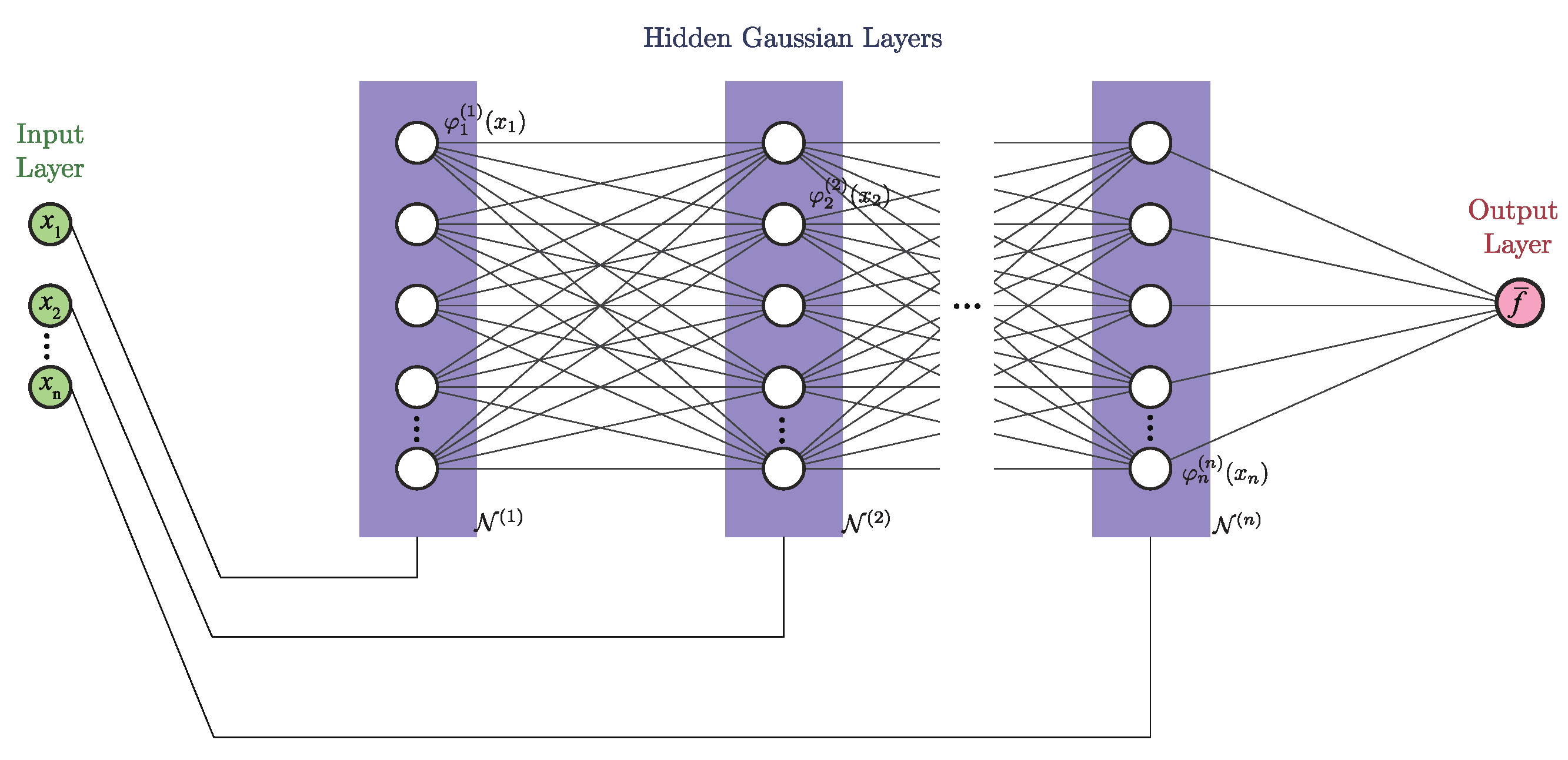
Given that the recent development of deep neural networks has shown promise in solving such problems, the main goal of this paper is to develop a deep-neural-network representation of GRBFNN or at least a good approximation of it with significant improvement of computational efficiency such that the network can be used for solving very high dimensional problems. We approach this problem by utilizing the separable property of Gaussian radial basis functions. That is, every Gaussian-radial-basis function can be decomposed into the product of multiple uni-variate Gaussian functions. Based on this property, we construct a new neural network, namely separable Gaussian neural network (SGNN), whose number of layers is equal to the number of input dimensions, with the neurons of each layer formed by the corresponding uni-variate Gaussian functions. Through dividing the input into multiple columns by their dimensions and feeding them into the corresponding layers, the output equivalent to that of a GRBFNN is constructed from multiplications and summations of uni-variate Gaussian functions in the forward propagation. It should be noted that Poggio and Girosi [15] have reported the separable property of Gaussian-radial-basis functions and proposed using it for neurobiology even in 1990.

SGNN offers several advantages.

• The number of neurons of SGNN is $O\left(dN\right)$ and increases linearly with the dimension of the input, while the number of neurons of GRBFNN given by $O\left(N^d\right)$ grows exponentially. This reduction in neurons also decreases the number of trainable variables from $O\left(N^d\right)$ to $O\left(d{N}^2\right)$, yielding a more compact network than GRBFNN.
• The reduction in trainable variables further decreases the computational load during the training and testing of neural networks. As shown in Section 3, this has led to 100 times speedup of training time for approximating tri-variate functions.
• SGNN is much easier to tune than other MLPs. Since the number of layers in SGNN is equal to the number of dimension of the input data, the only tunable network-structural hyper-parameter is the layer width, i.e., the number of neurons in a layer. This can significantly alleviate the tuning workload as compared to other MLPs that must simultaneously tune the width and depth of layers.
• SGNN holds a similar level of accuracy as GRBFNN, making it particularly suitable for approximating multi-variate functions with complex geometry. In Section 7, it is shown that SGNN can yield approximations for complex functions that are three orders of magnitude more accurate than those MLPs yield with ReLU and Sigmoid functions.

The rest of this paper is organized as follows. In Section 2, we introduce the structure of SGNN and use it to approximate a multi-variate real-value function. In Section 3, we compare SGNN and GRBFNN regarding the number of trainable variables and the computational complexity of forward and backward propagation. In Section 4, we show that SGNN can preserve the dominant sub-eigenspace of the Hessian of GRBFNN in the gradient descent search. This property can help SGNN maintain a similar level of accuracy as GRBFNN while substantially improving the computational efficiency. In Section 5, we show that the computational time of SGNN scales linearly with the increase in dimension and demonstrate its efficacy in function approximations through numerous examples. In Section 6 and Section 7, extensive comparisons between SGNN and GRBFNN and between SGNN and MLPs are performed. At last, the conclusion is summarized in Section 8.

2. Separable-Gaussian Neural Networks

Definition 1.

A d-variate function $f(x_1,x_2,\cdots ,x_d)$ is separable if it can be expressed as a product of multiple uni-variate functions; i.e.,

$$f(x_1,x_2,\cdots ,x_d)=f_1\left(x_1\right)·f_2\left(x_2\right)\cdots f_d\left(x_d\right).$$

(3)

Remark 1.

Recall that the Gaussian radial-basis function in Equation (2) is separable and can be represented in the form

$$G\left(\mathbf{x}\right)=\prod _{k=1}^d{\phi }^{\left(k\right)}\left(x_k\right),$$

(4)

where ${\phi }^{\left(k\right)}\left(x_k\right)=exp(-\frac{1}{2}{(x_k-{\mu }_k)}^2/{\sigma }_k^2)$, with $k=1,2,\cdots ,d$.

The product chain in Equation (4) can be constructed through the forward propagation of a feedforward network with a single neuron per layer where ${\phi }^{\left(k\right)}\left(x_k\right)$ is the neuron of the k-th layer. This way, the multi-variate Gaussian function $G\left(\mathbf{x}\right)$ is reconstructed at the output of the network. By adding more neurons to each layer and assigning weights to all edges, we can eventually construct a network whose output is equivalent to the output of a GRBFNN. Figure 1 shows an example of an SGNN approximating a tri-variate function. Next, we use this property to define SGNN.

Definition 2.

The separable-Gaussian neural network (SGNN) with d-dimensional input can be constructed in the form

$$\begin{array}{cc}\hfill {\mathcal{N}}_i^{\left(0\right)}& =x_i, 1\le i\le d,\hfill \end{array}$$

(5)

$$\begin{array}{cc}\hfill {\mathcal{N}}_i^{\left(1\right)}& ={\phi }_i^{\left(1\right)}(x_1,{\mu }_i^{\left(1\right)},{\sigma }_i^{\left(1\right)}), 1\le i\le N_1,\hfill \end{array}$$

(6)

$$\begin{array}{cc}\hfill {\mathcal{N}}_i^{(\ell )}& ={\phi }_i^{(\ell )}(x_{\ell },{\mu }_i^{(\ell )},{\sigma }_i^{(\ell )})\sum _{j=1}^{N_l}{W}_{ij}^{(\ell )}{\mathcal{N}}_j^{(\ell -1)}, 2\le \ell \le d,1\le i\le N_{\ell },\hfill \end{array}$$

(7)

$$\begin{array}{cc}\hfill \overline{f}\left(\mathbf{x}\right)& =\mathcal{N}\left(\mathbf{x}\right)=\sum _{j=1}^{N_d}{\mathcal{N}}_j^{\left(d\right)},\hfill \end{array}$$

(8)

where $N_i$ ($i=1,2,\cdots ,d$) represents the number of neurons of the l-th layer, ${\mathcal{N}}_i^{\left(l\right)}$ represents the output of the i-th Gaussian neuron (activation function) of the l-th layer. In addition, ${\mu }_i^{\left(l\right)}$, ${\sigma }_i^{\left(l\right)}$ represent the i-th center and width of the l-th layer, respectively.

The weights of the output layer are assumed to be unity, although they can be trainable. Substituting Equations (5)–(7) into Equation (8) yields

$$\overline{f}\left(\mathbf{x}\right)=\sum _{i_d=1}^{N_d}\sum _{i_{d-1}=1}^{N_{d-1}}\cdots \sum _{i_1=1}^{N_1}\left[W_{i_d{i}_{d-1}}^{(d-1)}{W}_{i_{d-1}{i}_{d-2}}^{(d-2)}\cdots W_{i_2{i}_1}^{\left(1\right)}\right]\prod _{\ell =1}^d{\phi }_{i_{\ell }}^{(\ell )}\left(x_{\ell }\right),$$

(9)

with

$$\prod _{\ell =1}^d{\phi }_{i_{\ell }}^{(\ell )}\left(x_{\ell }\right)={\phi }_{i_d}^{\left(d\right)}\left(x_d\right){\phi }_{i_{d-1}}^{(d-1)}\left(x_{d-1}\right)\cdots {\phi }_{i_1}^{\left(1\right)}\left(x_1\right),$$

(10)

where $W_{i_{l+1}{i}_l}^{\left(l\right)}$ ($l=1,2,\cdots ,d$) represents the weight of the $i_{(l+1)}$-th neuron of the $(l+1)$-th layer and the $i_l$-th neuron of the l-th layer. The loss function of the SGNN is defined in the form

$$J={\parallel f-\overline{f}\parallel }_2=\sqrt{\sum _{i=1}^d{\left[f\left(x_i\right)-\overline{f}\left(x_i\right)\right]}^2}.$$

(11)

The center ${\mu }_i^{\left(l\right)}$ and width ${\sigma }_i^{\left(l\right)}$ in the Gaussian function ${\phi }_i^{\left(l\right)}$ can also be treated as trainable. They are not included in this discussion for simplicity.

3. SGNN vs. GRBFNN

Without loss of generality, the analysis below will assume that each hidden layer has N neurons. To understand how the weights of SGNN relate to those of GRBFNN, we equate Equations (1) and (9), which yields a nonlinear map

$${\mathcal{W}}_j=g_j\left(W_{i_d{i}_{d-1}}^{(d-1)},W_{i_{d-1}{i}_{d-2}}^{(d-2)},\cdots ,W_{i_2{i}_1}^{\left(1\right)}\right),$$

(12)

whose explicit form is

$${\mathcal{W}}_j=W_{i_d{i}_{d-1}}^{(d-1)}{W}_{i_{d-1}{i}_{d-2}}^{(d-2)}\cdots W_{i_2{i}_1}^{\left(1\right)},$$

(13)

with

$$j=i_1+(i_2-1)N+\cdots +(i_d-1)N^{d-1}.$$

(14)

It is evident that SGNN can be transformed into GRBFNN. However, GRBFNN can be converted into SGNN if and only if the mapping of Equation (13) is invertible.

In general, SGNN would have much fewer parameters than GRBFNN, which means, for most possible GRFNN networks, there is no equivalent SGNN network with an identical set of centers and widths. It is unclear at this time whether SGNNs can form a dense sub-set of GRBFNNs. The aim of this paper is to show that SGNN can cost substantially less computational effort than GRBFNN but provide comparable (occasionally even greater) accuracy through extensive numerical experiments in modeling ten very different functions. In this regard, even if SGNNs cannot lead to an arbitrarily close approximation of GRBFFs, there is still value in using them for high-dimensional problems due to their computational efficiency. In addition, SGNNs can have superior performances in approximating complex functions rather than deep neural networks with activation functions such as ReLU and Sigmoid, as shown in Section 7.

In the following, we demonstrate the computational efficiency of SGNN over GRBFNN in terms of trainable variables and the number of floating-point operations of forward and backward propagation.

3.1. Trainable Variables

Let us now treat the center and width of the uni-variate Gaussian function in SGNN as trainable. The total number $N_t$ of trainable variables of SGNN is given by

$$N_t=\left\{\begin{array}{cc}N+2N\hfill & \mathbf{x}\in {\mathbb{R}}^1,\hfill \\ (d-1)N^2+2dN\hfill & \mathbf{x}\in {\mathbb{R}}^d, \mathrm{for} d\ge 2.\hfill \end{array}\right.$$

(15)

Note that the number of trainable variables of GRBFNN is $N^d$, identical to its number of neurons. SGNN and GRBFNN have identical weights when the number of layers is smaller than or equal to two. In other words, they are mutually convertible and the mapping of Equation (13) is invertible when $d\le 2$. However, for high-dimensional problems, as shown in

Table 1. Neurons and trainable variables of SGNN and GRBFNN.

	Neurons	No. of Variables
SGNN	$O\left(dN\right)$	$O\left(d{N}^2\right)$
GRBFNN	$O\left(N^d\right)$	$O\left(N^d\right)$

, SGNN can substantially reduce the number of trainable variables, making it more tractable than GRBFNN.

3.2. Forward Propagation

Assume the size of the input dataset is m. Using Equations (5) to (8), we can estimate the number of floating-point operations (FLOPs) of the forward pass in SGNNs. More specifically, the number of FLOPs to calculate the output of the k-th layer with the input from the previous layer is

$$FLO{P}^{\left(k\right)}\left(\mathcal{N}\left(\mathbf{x}\right)\right)=m(2N^2+6N), \mathrm{for} 2\le k\le d,$$

(16)

where $2N^2$ is the number of arithmetic operations by the product of weights and Gaussian functions of the k-th layer, $6N$ is the number of calculations for Gaussian functions of the layer, and m is the size of input dataset. In addition, the numbers of FLOPs associated with the first and output layer are

$$\begin{array}{c}\hfill FLO{P}^{\left(1\right)}\left(\mathcal{N}\left(\mathbf{x}\right)\right)=6mN,\end{array}$$

(17)

$$\begin{array}{c}\hfill FLO{P}^{(d+1)}\left(\mathcal{N}\left(\mathbf{x}\right)\right)=mN.\end{array}$$

(18)

Therefore, the total number of FLOPs is

$$O\left(FLO{P}_{fp}\right)=O\left(\sum _{i=1}^{d+1}FLO{P}^{\left(i\right)}\right)=O\left(md{N}^2\right).$$

(19)

The number of operations increases linearly with the increase in the number of layers or the dimension of the input vector d. On the other hand, the computational complexity of FLOP of RBGNN is

$$O\left(FLO{P}_{\widetilde{fp}}\right)=O\left(m{N}^d\right),$$

(20)

regardless of the trainability of the centers and width of Gaussian functions.

3.3. Backward Propagation

Accurately estimating the computational complexity of backward propagation is challenging because techniques such as autodifferentiation [28] and computational graphs [26] have optimized the original mathematical operations for improving the computational performance. Autodifferentiation evaluates the derivative of numerical functions using dual numbers with the chain rule broken into a sequence of operations such as addition, multiplication, and composition. During forward propagation, intermediate values in computational graphs are recorded for backward propagation.

We analyze the operations of backward propagation with respect to a single neuron of the l-th layer. The partial derivatives of $\overline{f}\left(\mathbf{x}\right)$ with respect to ${\mathcal{W}}_j^{\left(l\right)}$, ${\mu }_j^{\left(l\right)}$, and ${\sigma }_j^{\left(l\right)}$ of the l-th ($1\le l\le d$) layer in SGNN are

$$\begin{array}{cc}\hfill \frac{\partial \overline{f}}{\partial {\mathcal{W}}_j^{\left(l\right)}}& ={\left[\frac{\partial \overline{f}}{\partial {\mathcal{N}}_j^{(l+1)}}\right]}^T\frac{\partial {\mathcal{N}}_j^{(l+1)}}{\partial {\mathcal{W}}_j^{\left(l\right)}},\hfill \end{array}$$

(21)

$$\begin{array}{cc}\hfill \frac{\partial \overline{f}}{\partial {\mu }_j^{\left(l\right)}}& ={\left[\frac{\partial \overline{f}}{\partial {\mathcal{N}}_j^{(l+1)}}\right]}^T\frac{\partial {\mathcal{N}}_j^{(l+1)}}{\partial {\mu }_j^{\left(l\right)}},\hfill \end{array}$$

(22)

$$\begin{array}{cc}\hfill \frac{\partial \overline{f}}{\partial {\sigma }_j^{\left(l\right)}}& ={\left[\frac{\partial \overline{f}}{\partial {\mathcal{N}}_j^{(l+1)}}\right]}^T\frac{\partial {\mathcal{N}}_j^{(l+1)}}{\partial {\sigma }_j^{\left(l\right)}},\hfill \end{array}$$

(23)

with

$$\left[\frac{\partial \overline{f}}{\partial {\mathcal{N}}_j^{(l+1)}}\right]={\left[\frac{\partial \overline{f}}{\partial {\mathcal{N}}^{(l+2)}}\right]}^T\left[\frac{\partial {\mathcal{N}}^{(l+2)}}{\partial {\mathcal{N}}_j^{(l+1)}}\right],$$

(24)

where

$${\mathcal{N}}^{(l+2)}={({\mathcal{N}}_1^{(l+2)},{\mathcal{N}}_2^{(l+2)},\cdots ,{\mathcal{N}}_N^{(l+2)})}^T.$$

(25)

The backward prorogation with respect to the j-th neuron of the l-th ($1\le l\le n-1$) layer can be divided into three steps:

• Compute the gradient of $\overline{f}$ with respect to the output of the first neuron in the $(l+1)$-th layer, ${\mathcal{N}}_j^{(l+1)}$, as shown in Equation (24), where ${\left[\frac{\partial \overline{f}}{\partial {\mathcal{N}}^{(l+2)}}\right]}^T$ can be accessed from the back propagation of the $(l+2)$-th layer. This leads to $2N$ FLOP due to the dot product of two vectors.
• Calculate the partial derivatives of ${\mathcal{N}}_j^{(l+1)}$ with respect to weights, center, and width. Since the calculation of derivatives is computationally cheap, the analysis below will neglect the operations used to evaluate derivatives. This shall not affect the conclusion.
• Propagate the gradients backward. This produces $N+2$ operations.

Therefore, the number of FLOPs of the l-th layer is approximately $m(3N^2+2N)$, where m is the volume of the input dataset. The backward propagation of the last layer leads to N operations. In total, the number of FLOPs by backward propagation is

$$O\left(FLO{P}_{bp}\right)=O\left(md{N}^2\right).$$

(26)

On the other hand, the backward propagation FLOP number of GRBFNN is

$$O\left(FLO{P}_{\widetilde{bp}}\right)=O\left(m{N}^d\right).$$

(27)

4. Subspace Gradient Descent

The aim of this section is to discuss the high performances of SGNNs over GRBFNNs in terms of computational efficiency and accuracy through the lens of gradient descent. As illustrated in Section 3, SGNN has exponentially fewer trainable variables than the associated GRBFNN for high-dimensional input. In other words, GRBFNN may be over-parameterized. The recent work [29,30,31] has shown that optimizing a loss function constructed by an over-parameterized neural network can lead to Hessian matrices that possess few dominant eigenvalues with many near-zero ones before and after training. This means the gradient descent can happen in a small subspace. Inspired by their work, we consider the infinitesimal variation of the loss function J for GRBFNN a

$$dJ={\left[\frac{\partial J}{\partial \tilde{\mathit{\theta }}}\right]}^{T}d\tilde{\mathit{\theta }}+\frac{1}{2}d{\tilde{\mathit{\theta }}}^T\tilde{H}d\tilde{\mathit{\theta }}+h.o.t.\left({\parallel d\tilde{\mathit{\theta }}\parallel }^3\right),$$

(28)

where $\tilde{\mathit{\theta }}$ represents a vector of all trainable weights, and

$$\tilde{\mathbf{H}}=\frac{{\partial }^{2}J}{\partial {\tilde{\mathit{\theta }}}^T\tilde{\mathit{\theta }}},$$

(29)

is the associated Hessian matrix. The centers and widths of Gaussian functions are assumed to be constant for simplicity. Since the Hessian matrix $\tilde{H}$ is symmetric, we can represent it in the form

$$\tilde{\mathbf{H}}={\mathbf{P}}^T\left(\begin{array}{cc}{\mathit{\lambda }}_d& \mathbf{0}\\ \mathbf{0}& {\mathit{\lambda }}_s\end{array}\right)\mathbf{P},$$

(30)

where ${\mathit{\lambda }}_d=\mathrm{diag}({\lambda }_1,{\lambda }_2,\cdots ,{\lambda }_k,\cdots ,{\lambda }_{dN})$ are the k dominant eigenvalues padded by $(dN-k)$ non-dominant ones (assuming $k<dN$), and ${\mathit{\lambda }}_s$ = $\mathrm{diag}({\lambda }_{dN+1},{\lambda }_{dN+2},\cdots ,{\lambda }_{N^d})$ are the rest non-dominant eigenvalues.

Let $\mathit{\theta }$ be the weights of SGNN. The variation of the mapping from $\mathit{\theta }$ to $\tilde{\mathit{\theta }}$ in Equation (12) reads

$$d\tilde{\mathit{\theta }}=\frac{\partial \mathbf{g}}{\partial \mathit{\theta }}d\mathit{\theta },$$

(31)

where $\frac{\partial \mathbf{g}}{\partial \mathit{\theta }}$: ${\mathbb{R}}^{dN}\mapsto {\mathbb{R}}^{N^d\times dN}$. It should be noted that $\frac{\partial \mathbf{g}}{\partial \mathit{\theta }}$ is a super sparse matrix.

Substitution of Equation (31) into Equation (28)

$$dJ={\left[\frac{\partial J}{\partial \tilde{\mathit{\theta }}}\right]}^T\frac{\partial \mathbf{g}}{\partial \mathit{\theta }}d\mathit{\theta }+\frac{1}{2}d{\mathit{\theta }}^T\mathbf{H}d\mathit{\theta }+h.o.t.\left({\parallel d\tilde{\mathit{\theta }}\parallel }^3\right),$$

(32)

with

$$\begin{array}{cc}\hfill \mathbf{H}& ={\left[\frac{\partial \mathbf{g}}{\partial \mathit{\theta }}\right]}^T\tilde{\mathbf{H}}\frac{\partial \mathbf{g}}{\partial \mathit{\theta }}\hfill \\ & ={\left[\frac{\partial \mathbf{g}}{\partial \mathit{\theta }}\right]}^T{\mathbf{P}}^T\left(\begin{array}{cc}{\mathit{\lambda }}_d& \mathbf{0}\\ \mathbf{0}& {\mathit{\lambda }}_s\end{array}\right)\mathbf{P}\left[\frac{\partial \mathbf{g}}{\partial \mathit{\theta }}\right].\hfill \end{array}$$

(33)

Let

$$\left(\begin{array}{c}{\mathbf{Q}}_d\\ {\mathbf{Q}}_s\end{array}\right)=\mathbf{P}\left[\frac{\partial \mathbf{g}}{\partial \mathit{\theta }}\right],$$

(34)

where ${\mathbf{Q}}_d\in {\mathbb{R}}^{dN\times dN}$ and ${\mathbf{Q}}_s\in {\mathbb{R}}^{(N^d-dN)\times dN}$. Substituting Equation (34) into Equation (33) yields

$$\begin{array}{cc}\hfill \mathbf{H}& ={\mathbf{Q}}_d^T{\mathit{\lambda }}_d{\mathbf{Q}}_d+{\mathbf{Q}}_s^T{\mathit{\lambda }}_s{\mathbf{Q}}_s\approx {\mathbf{Q}}_d^T{\mathit{\lambda }}_d{\mathbf{Q}}_d.\hfill \end{array}$$

(35)

Therefore, the dominant eigenvalues of the Hessian of GRBFNN are also included in the corresponding SGNN. This means that the gradient of SGNN can descend in the mapped dominant non-flat subspace of GRBFNN, which may contribute to the comparable accuracy and training efficiency of SGNN as opposed to GRBFNN, as discussed in Section 3.

5. Numerical Experiments

5.1. Candidate Functions

We consider ten candidate functions from [32,33] and modified them, as listed in

Table 2. Candidate functions and their features.

Functions	Features	Explicit Expression
Root sum squared	Sink	$f_1\left(\mathbf{x}\right)={\left({\sum }_{i=1}^d{x}_i^2\right)}^{\frac{1}{2}}$
Second-degree polynomial	Saddle	$f_2\left(\mathbf{x}\right)=\frac{1}{50}{\sum }_{j=1}^d{x}_j^2{x}_{j+1}$
Exponential-square sum	Flatter sink	$f_3\left(\mathbf{x}\right)=\frac{1}{5}{\sum }_{j=1}^d{e}^{x_j^2/50}$
Exponential-sinusoid sum	Sink and source	$f_4\left(\mathbf{x}\right)=\frac{1}{5}{\sum }_{j=1}^d{e}^{x_j^2/50}sin\left(y_j\right)$
Polynomial-sinusoid sum	Sink and source	$f_5\left(\mathbf{x}\right)=\frac{1}{50}{\sum }_{j=1}^d{x}_j^{2}cos(j\ast x_j)$
Inverse-exponential-square sum	Source	$f_6\left(\mathbf{x}\right)=10/{\sum }_{j=1}^d{e}^{x_j^2/25}$
Sigmoidal	S-shaped surface	$f_7\left(\mathbf{x}\right)=10/(1+e^{-\frac{1}{5}{\sum }_{i=1}^d{x}_j})$
Gaussian	Flatter source	$f_8\left(\mathbf{x}\right)=10e^{-\frac{1}{100}{\sum }_{j=1}^5{x}_j^2}$
Linear	Flat	$f_9\left(\mathbf{x}\right)={\sum }_{j=1}^d{x}_j$
Constant	Flat	$f_{10}\left(\mathbf{x}\right)=1$

Note: In $f_4$, $y_j=x_{j+1}$ with $j=1,2,\cdots ,d-1$ and $y_d=x_1$.

. The functions cover a range of distinct features, including sinks, sources, flat and s-shaped surfaces, and multiple sinks and sources, which can assist in benchmarking the function approximations of different neural networks.

We generate uniformly distributed sample sets to train neural networks for each run, with the upper and lower bounds of each dimension ranging from −8 to 8. The initial centers of Gaussian functions are evenly distributed in each dimension and widths are the distance of two adjacent centers. During the training process, we employ mini-batch gradient descent with the optimizer Adam in Tensorflow to update model parameters. The optimizer uses its default training parameters and stops if no improvement of loss values is achieved in four consecutive epochs. The dataset is divided into a training set comprising 80% of the data and a validation set consisting of the remaining 20%. The mini-batch size, number of neurons, and data points are selected to balance the convergence speed and accuracy. All tests are performed on a Windows-10 desktop with a 3.6 HZ, 8-core, Intel i7-9700K CPU and a 64 GB Samsung DDR-3 RAM.

5.2. Dimension Scalability

In order to understand the dimensional scalability of SGNN, we applied SGNN to candidate functions with the number of dimensions from two to five, as presented in

Table 3. The computation time of SGNN per epoch scales linearly with the increase in dimensions. Data are generated by averaging the results of 30 runs. Data Size: 16,384, Mini-batch size: 256. Neurons per layer: 20.

	2D		3D		4D		5D
	Seconds/Epoch	Loss	Seconds/Epoch	Loss	Seconds/Epoch	Loss	Seconds/Epoch	Loss
$f_1$	0.065	$2.31\times {10}^{-4}$	0.081	$4.43\times {10}^{-4}$	0.099	$1.41\times {10}^{-3}$	0.113	$4.43\times {10}^{-4}$
$f_2$	0.063	$7.34\times {10}^{-5}$	0.081	$8.31\times {10}^{-4}$	0.098	$2.50\times {10}^{-3}$	0.114	$8.31\times {10}^{-4}$
$f_3$	0.064	$4.26\times {10}^{-6}$	0.083	$1.50\times {10}^{-5}$	0.106	$4.13\times {10}^{-5}$	0.110	$1.50\times {10}^{-5}$
$f_4$	0.065	$2.80\times {10}^{-6}$	0.084	$2.91\times {10}^{-5}$	0.100	$9.12\times {10}^{-5}$	0.108	$2.91\times {10}^{-5}$
$f_5$	0.063	$7.40\times {10}^{-5}$	0.083	$7.53\times {10}^{-4}$	0.099	$1.00\times {10}^{-1}$	0.107	$7.53\times {10}^{-4}$
$f_6$	0.063	$1.39\times {10}^{-6}$	0.083	$1.27\times {10}^{-5}$	0.101	$2.11\times {10}^{-5}$	0.115	$1.27\times {10}^{-5}$
$f_7$	0.063	$4.44\times {10}^{-5}$	0.083	$4.08\times {10}^{-4}$	0.099	$1.89\times {10}^{-3}$	0.111	$4.08\times {10}^{-4}$
$f_8$	0.063	$1.97\times {10}^{-5}$	0.083	$4.36\times {10}^{-5}$	0.100	$7.76\times {10}^{-5}$	0.113	$4.36\times {10}^{-5}$
$f_9$	0.063	$2.27\times {10}^{-4}$	0.079	$1.76\times {10}^{-3}$	0.099	$9.93\times {10}^{-3}$	0.111	$1.76\times {10}^{-3}$
$f_{10}$	0.064	$3.51\times {10}^{-6}$	0.082	$6.32\times {10}^{-6}$	0.101	$9.84\times {10}^{-6}$	0.113	$6.32\times {10}^{-6}$

. For comparison, the data points were kept as 16,384 such that sufficient data were sampled for 5D functions, i.e., $d=5$. Each layer has fixed 20 uni-variate Gaussian neurons, with initial centers evenly distributed in each dimension and widths being the distance between two adjacent centers. The training time per epoch grows linearly as the dimension increases, with an increment of 0.02 s/epoch per layer. For the majority of candidate functions, SGNN can achieve the accuracy level of ${10}^{-4}$. It is sufficient to approximate the 5D functions by SGNN with five layers and a total of 100 neurons. The configuration of SGNN cannot effectively approximate the function $f_5$ in 4D. This can be easily resolved by adding more neurons into the neural network (see a similar example in Table 7). In summary, the computational time of SGNN scales linearly with the increase in dimensions.

Then, 2D and 5D examples are selected to illustrate the expressiveness of SGNN in function approximations. The number of neurons, training size, and mini-batch size are fine-tuned to achieve optimal results.

5.3. Two-Dimensional Examples

First, SGNN is used to approximate the two-dimension function $f_3\left(\mathbf{x}\right)=1/5e^{(x_1^2+x_2^2)/50}$, which has four sharp peaks and one flat valley in the domain. As illustrated in Figure 2a, the optimizer converges in 400 steps, with the difference between training and test sets at the magnitude level of ${10}^{-4}$. Figure 2b–e show that the prediction by SGNN is nearly identical to the ground truth, except for the domain near boundaries. This can be attributed to fewer sampling points in the neighborhood of the boundaries. Better alignment can be achieved by sampling extra boundary points to the input dataset.

SGNN maintains its level of accuracy as candidate functions become more complex. For example, Figure 3 presents the approximation of $f_4\left(\mathbf{x}\right)=\frac{1}{5}(e^{x_1^2/50}sin{x}_2+e^{x_2^2/50}sin{x}_1)$. SGNN can approximate $f_4$ with the same level of accuracy as $f_3$ even with fewer training epochs, possibly led by the localization property of Gaussian function. The largest error again appears near boundaries, with a percentage error less than 8%. Inside the domain, the computed values precisely match the exact ones. As visualized in Figure 3d,e, the prediction by SGNN can fully capture the features of the function.

This finding is corroborated in Figure 4, which presents the approximation of the function $f_5\left(\mathbf{x}\right)=\frac{1}{50}(x_1^{2}cos{x}_1+x_2^{2}cos2x_2)$ by SGNN. The function, different from $f_4$, possesses peaks and valleys near boundaries and becomes flat in the vicinity of origin, as illustrated in Figure 4c–e. Interestingly, the neural network converges faster than the network for $f_4$. This indicates that the loss function may become more convex and contain fewer flat regions. One possible reason is that, as the function becomes more complex, more Gaussian neurons are active and have larger weights, increasing the loss gradients. The largest error is again observed near boundaries. As shown in Figure 4, SGNN can capture the features of the target function $f_5$. Due to the gradient configuration of the color bar, the small offset with respect to the ground truth occurs near the origin, but the corresponding absolute errors are very small, as shown in Figure 4b.

5.4. Five-Dimensional Examples

The approximation of five-dimensional functions from $f_1$ to $f_{10}$ by SGNN is illustrated through cross-sectional plots in the $x_1-x_2$ plane with three other variables fixed to zero, as shown in Figure 5 and Figure 6. The left panel is for prediction, and the right panel is for ground truth. During training, uniformly sampled training sets with the size of 32,768 were separately generated for all functions in order to maintain consistency. However, fewer points can be used when the function shape is simple (e.g., sink or source). The validation set used to produce the prediction plots is generated by uniformly partitioning the subspace with a step size twice the number of neurons per layer.

The SGNN can accurately capture the features of all candidates regardless of their geometric complexity. Although the predictions of SGNN show minor disagreements with the ground truth when the function (e.g., $f_{10}$) is constant, the differences are less than 3%.

6. Comparison of SGNN and GRBFNN

The performances of SGNN and GRBFNN in approximating two-dimensional and three-dimensional candidate functions are presented in

Table 4. Two-dimensional function approximations using SGNN and GRBFNN. Data are generated by averaging the results of 30 runs. Sample points: 1024; mini-batch size: 64; neurons per layer: 10.

	SGNN				GRBFNN
	Epoch	Seconds/Epoch	Ave Loss	Min Loss	Epoch	Seconds/Epoch	Ave Loss	Min Loss
$f_1$	483	0.027	$1.86\times {10}^{-3}$	$1.32\times {10}^{-3}$	568	0.232	$1.98\times {10}^{-4}$	$1.25\times {10}^{-4}$
$f_2$	333	0.028	$6.51\times {10}^{-5}$	$3.65\times {10}^{-5}$	351	0.199	$2.17\times {10}^{-5}$	$1.35\times {10}^{-5}$
$f_3$	334	0.027	$1.32\times {10}^{-5}$	$6.44\times {10}^{-6}$	349	0.193	$6.21\times {10}^{-6}$	$2.30\times {10}^{-6}$
$f_4$	223	0.028	$7.12\times {10}^{-6}$	$5.53\times {10}^{-6}$	209	0.194	$4.62\times {10}^{-6}$	$2.68\times {10}^{-6}$
$f_5$	123	0.030	$3.72\times {10}^{-6}$	$1.82\times {10}^{-6}$	126	0.198	$1.99\times {10}^{-6}$	$1.15\times {10}^{-6}$
$f_6$	595	0.027	$2.41\times {10}^{-4}$	$1.50\times {10}^{-4}$	629	0.209	$7.41\times {10}^{-5}$	$3.20\times {10}^{-5}$
$f_7$	602	0.027	$6.17\times {10}^{-4}$	$4.93\times {10}^{-4}$	636	0.192	$1.77\times {10}^{-4}$	$8.24\times {10}^{-5}$
$f_8$	822	0.026	$3.62\times {10}^{-4}$	$2.70\times {10}^{-4}$	756	0.191	$3.48\times {10}^{-4}$	$1.56\times {10}^{-4}$
$f_9$	625	0.026	$8.56\times {10}^{-4}$	$4.38\times {10}^{-4}$	591	0.190	$4.84\times {10}^{-4}$	$1.45\times {10}^{-4}$
$f_{10}$	437	0.026	$2.97\times {10}^{-5}$	$2.26\times {10}^{-5}$	444	0.199	$1.09\times {10}^{-5}$	$6.15\times {10}^{-6}$

and

Table 5. Approximations of tri-variate functions using SGNN and GRBFNN. SGNN can achieve an acceleration 100-fold that of GRBFNN, with even smaller loss values for the functions $f_3$–$f_5$ (highlighted). Data were generated by averaging the results of 30 runs. Sample points: 2048; mini-batch size: 64; Neurons per layer: 10.

	SGNN				GRBFNN
	Epoch	Seconds/Epoch	Ave Loss	Min Loss	Epoch	Seconds/Epoch	Ave Loss	Min Loss
$f_1$	269	0.038	$1.42\times {10}^{-3}$	$9.33\times {10}^{-4}$	270	4.049	$1.65\times {10}^{-4}$	$9.60\times {10}^{-5}$
$f_2$	253	0.039	$2.47\times {10}^{-4}$	$1.02\times {10}^{-4}$	157	4.055	$4.75\times {10}^{-5}$	$3.51\times {10}^{-5}$
$f_3$	204	0.039	$2.36\times {10}^{-5}$	$1.78\times {10}^{-5}$	164	4.068	$2.37\times {10}^{-5}$	$1.80\times {10}^{-5}$
$f_4$	188	0.039	$1.82\times {10}^{-5}$	$1.24\times {10}^{-5}$	97	4.077	$1.96\times {10}^{-5}$	$1.61\times {10}^{-5}$
$f_5$	150	0.040	$2.72\times {10}^{-6}$	$1.44\times {10}^{-6}$	66	4.169	$1.56\times {10}^{-5}$	$1.20\times {10}^{-5}$
$f_6$	323	0.037	$7.20\times {10}^{-5}$	$4.29\times {10}^{-5}$	245	4.085	$3.75\times {10}^{-5}$	$2.73\times {10}^{-5}$
$f_7$	324	0.037	$1.16\times {10}^{-3}$	$7.07\times {10}^{-4}$	274	4.031	$1.65\times {10}^{-4}$	$1.02\times {10}^{-4}$
$f_8$	315	0.036	$1.95\times {10}^{-3}$	$8.48\times {10}^{-4}$	314	3.937	$2.03\times {10}^{-4}$	$1.41\times {10}^{-4}$
$f_9$	334	0.036	$4.29\times {10}^{-3}$	$1.89\times {10}^{-3}$	293	4.016	$7.60\times {10}^{-4}$	$4.96\times {10}^{-4}$
$f_{10}$	227	0.038	$3.28\times {10}^{-5}$	$2.45\times {10}^{-5}$	188	4.018	$2.63\times {10}^{-5}$	$1.72\times {10}^{-5}$

, respectively. For comparison, the centers and width of Gaussian neurons of GRBFNN are set to be trainable variables as well. We focus on the differences of total epochs, training time per epoch, and losses for comparison. The results are obtained by averaging the results of 30 runs.

As shown in Table 4, when approximating two-dimensional functions, SGNN can achieve comparable accuracy as GRBFNN, with differences of less than one-order-of magnitude in most cases. The worst case occurs with approximating $f_1$. However, the absolute difference is around $1.0\times {10}^{-3}$, and SGNN can still give a reasonably good approximation. On the other hand, the training time per epoch of SGNN is roughly one-tenth of that of GRBFNN.

The advantage of SGNN becomes more evident in three-dimensional function approximations. SGNN can gain a one-hundred-time speedup over GRBFNN but still maintain a similar level of accuracy. Surprisingly, SGNN can also yield more accurate results when approximating $f_3$ to $f_6$.

7. Comparison with Deep NNs

In this section, we compare the performance of SGNN with deep ReLU and Sigmoid NNs, which are two popular choices of activation functions. Through the approximation of four-dimensional candidate functions, SGNN shows much better trainability and approximability over deep ReLU and Sigmoid NNs.

Table 6 presents the training time per epoch, total epoch for training, and loss after training of three deep NNs by averaging the results of 30 runs. All NNs possess four hidden layers with 20 neurons per layer. The training-set size is fixed to 16,384, with a mini-batch size of 256. As opposed to SGNN and Sigmoid-NN, which have stable training times per epoch across all candidate functions, the time of ReLU-NN fluctuates. This might be led by the difference in calculating the derivatives of a ReLU unit with an input less or greater than zero. SGNN has a longer training time per epoch because of the computation of a Gaussian function and derivative of $\mu$ and $\sigma$. One may argue that this comparison is unfair because SGNN has extra trainable variables. However, SGNN has fewer trainable weights (see Table 7) because no weights connect the input and first layer, and the output layer is not trainable.

Table 6. Performance comparison of SGNN and deep neural networks with ReLU and Sigmoid activation functions. Data are generated by averaging the results of 30 runs. All NNs have four hidden layers, with 20 neurons per layer.

	SGNN			ReLU-NN			Sigmoid-NN
	Seconds/Epoch	Epoch	Loss	Seconds/Epoch	Epoch	Loss	Seconds/Epoch	Epoch	Loss
$f_1$	0.099	218	$1.41\times {10}^{-3}$	0.054	150	$4.86\times {10}^{-3}$	0.063	39	$4.78\times {10}^{-1}$
$f_2$	0.098	262	$2.50\times {10}^{-3}$	0.054	119	$1.07\times {10}^{-1}$	0.054	166	$2.90\times {10}^{-1}$
$f_3$	0.106	193	$4.13\times {10}^{-5}$	0.312	167	$5.22\times {10}^{-4}$	0.054	169	$1.30\times {10}^{-3}$
$f_4$	0.100	196	$9.12\times {10}^{-5}$	0.234	161	$7.32\times {10}^{-2}$	0.056	101	$2.38\times {10}^{-1}$
$f_5$	0.097	392	$9.65\times {10}^{-2}$	0.173	94	$4.97\times {10}^{-1}$	0.066	29	$6.38\times {10}^{-1}$
$f_6$	0.101	147	$2.11\times {10}^{-5}$	0.293	115	$1.18\times {10}^{-3}$	0.053	187	$2.94\times {10}^{-3}$
$f_7$	0.099	246	$1.89\times {10}^{-3}$	0.241	139	$2.07\times {10}^{-3}$	0.054	145	$1.58\times {10}^{-5}$
$f_8$	0.100	173	$7.76\times {10}^{-5}$	0.344	109	$9.95\times {10}^{-3}$	0.054	243	$3.17\times {10}^{-3}$
$f_9$	0.099	245	$9.93\times {10}^{-3}$	0.439	126	$7.66\times {10}^{-3}$	0.054	374	$7.79\times {10}^{-3}$
$f_{10}$	0.101	158	$9.84\times {10}^{-6}$	0.135	143	$6.86\times {10}^{-6}$	0.054	173	$8.20\times {10}^{-8}$

Table 6. Performance comparison of SGNN and deep neural networks with ReLU and Sigmoid activation functions. Data are generated by averaging the results of 30 runs. All NNs have four hidden layers, with 20 neurons per layer.

	SGNN			ReLU-NN			Sigmoid-NN
	Seconds/Epoch	Epoch	Loss	Seconds/Epoch	Epoch	Loss	Seconds/Epoch	Epoch	Loss
$f_1$	0.099	218	$1.41\times {10}^{-3}$	0.054	150	$4.86\times {10}^{-3}$	0.063	39	$4.78\times {10}^{-1}$
$f_2$	0.098	262	$2.50\times {10}^{-3}$	0.054	119	$1.07\times {10}^{-1}$	0.054	166	$2.90\times {10}^{-1}$
$f_3$	0.106	193	$4.13\times {10}^{-5}$	0.312	167	$5.22\times {10}^{-4}$	0.054	169	$1.30\times {10}^{-3}$
$f_4$	0.100	196	$9.12\times {10}^{-5}$	0.234	161	$7.32\times {10}^{-2}$	0.056	101	$2.38\times {10}^{-1}$
$f_5$	0.097	392	$9.65\times {10}^{-2}$	0.173	94	$4.97\times {10}^{-1}$	0.066	29	$6.38\times {10}^{-1}$
$f_6$	0.101	147	$2.11\times {10}^{-5}$	0.293	115	$1.18\times {10}^{-3}$	0.053	187	$2.94\times {10}^{-3}$
$f_7$	0.099	246	$1.89\times {10}^{-3}$	0.241	139	$2.07\times {10}^{-3}$	0.054	145	$1.58\times {10}^{-5}$
$f_8$	0.100	173	$7.76\times {10}^{-5}$	0.344	109	$9.95\times {10}^{-3}$	0.054	243	$3.17\times {10}^{-3}$
$f_9$	0.099	245	$9.93\times {10}^{-3}$	0.439	126	$7.66\times {10}^{-3}$	0.054	374	$7.79\times {10}^{-3}$
$f_{10}$	0.101	158	$9.84\times {10}^{-6}$	0.135	143	$6.86\times {10}^{-6}$	0.054	173	$8.20\times {10}^{-8}$

Table 7. Comparison of SGNN and ReLU-based NN in approximation of $f_5.$ Results are generated by averaging the data of 30 runs.

	Layers	Neuron/Layer	Parameters	Seconds/Epoch	Epoch	Loss	Min Loss
SGNN	4	20	1360	0.097	392	$9.65\times {10}^{-2}$	$3.91\times {10}^{-2}$
	4	40	5120	0.130	149	$7.08\times {10}^{-4}$	$5.32\times {10}^{-4}$
ReLU-NN	4	20	1381	0.056	96	0.497	0.477
	4	40	5161	0.067	99	0.458	0.409
	7	40	10,081	0.082	135	0.336	0.273
	10	40	15,001	0.176	112	0.324	0.258
	10	50	23,251	0.156	100	0.309	0.253
	10	60	33,301	0.250	96	0.288	0.232
	10	70	45,151	0.120	97	0.278	0.215
	10	80	58,801	0.261	89	0.291	0.205

Table 7. Comparison of SGNN and ReLU-based NN in approximation of $f_5.$ Results are generated by averaging the data of 30 runs.

	Layers	Neuron/Layer	Parameters	Seconds/Epoch	Epoch	Loss	Min Loss
SGNN	4	20	1360	0.097	392	$9.65\times {10}^{-2}$	$3.91\times {10}^{-2}$
	4	40	5120	0.130	149	$7.08\times {10}^{-4}$	$5.32\times {10}^{-4}$
ReLU-NN	4	20	1381	0.056	96	0.497	0.477
	4	40	5161	0.067	99	0.458	0.409
	7	40	10,081	0.082	135	0.336	0.273
	10	40	15,001	0.176	112	0.324	0.258
	10	50	23,251	0.156	100	0.309	0.253
	10	60	33,301	0.250	96	0.288	0.232
	10	70	45,151	0.120	97	0.278	0.215
	10	80	58,801	0.261	89	0.291	0.205

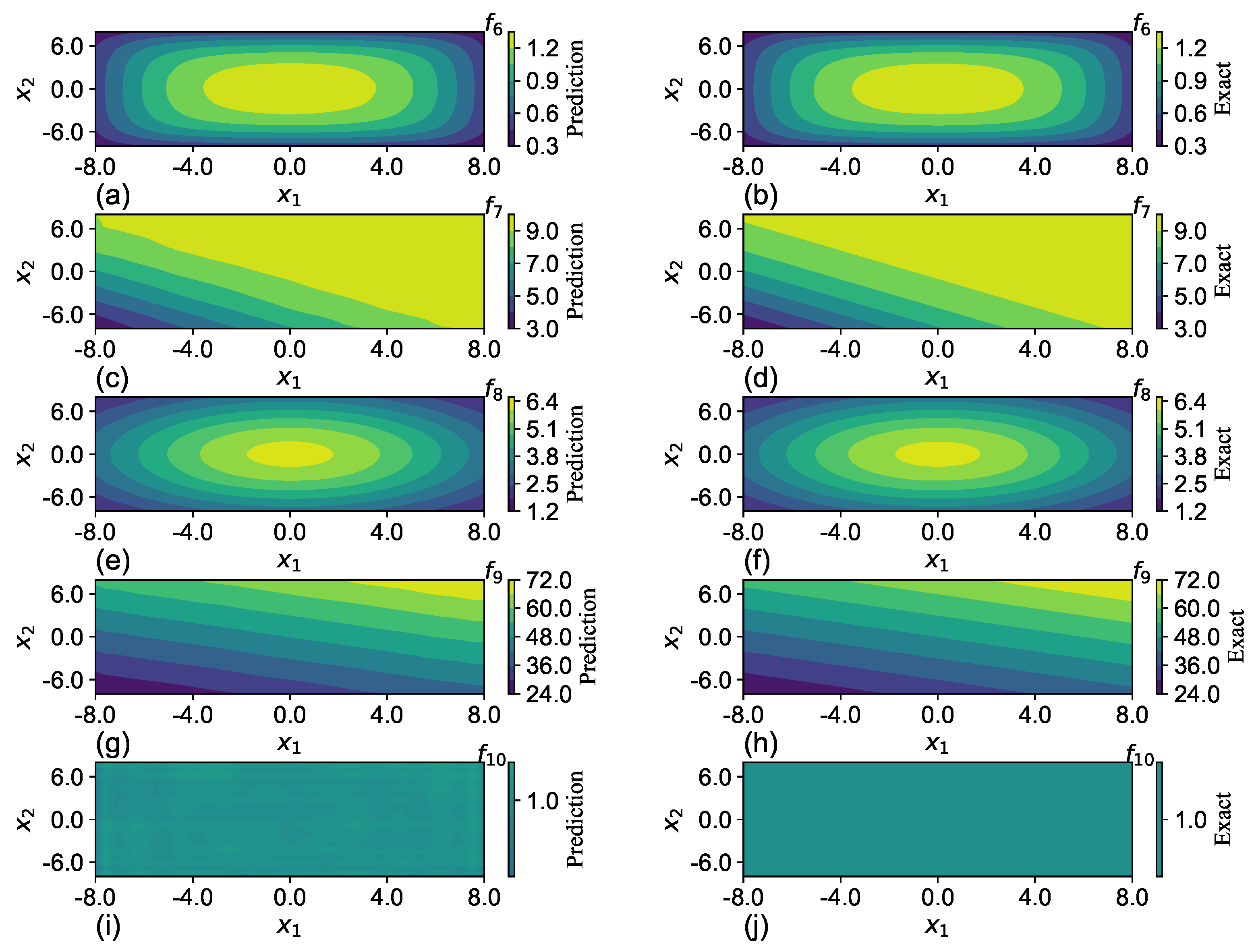
Although SGNN has appreciably larger training epochs, this also leads to more accurate predictions. The loss values of SGNN after training are uniformly smaller than those of ReLU-NN and Sigmoid-NN, except for $f_{10}$. In fact, for $f_2$, $f_4$, $f_6$, and $f_7$, the accuracy of SGNN is even two orders of magnitude better than the other two models.

Despite the efficient training speed of Sigmoid-NN, the network is more difficult to train with random weight initialization for $f_1$ and $f_5$. In fact, the approximation of $f_5$ by Sigmoid-NN is nowhere close to the group truth after training. When functions become more complex, SGNN outperforms ReLU-NN and Sigmoid-NN in minimizing loss through stochastic gradient descent. This could be attributed to the locality of Gaussian functions that increase the active neurons, reducing the flat subspace whose gradients diminish. Sigmoid-NN aborts with significantly fewer epoch numbers. This could be led by the small derivatives of Sigmoid functions when input stays within the saturation region, which makes it more difficult to train the network.

Next, we further compare the trainability of SGNN with ReLU-DNN. We train the two networks with different configurations to approximate the function $f_5$, which has a more complex geometry and is more difficult to approximate. The configuration of the NNs and the training performance are listed in Table 7.

Because the layer of SGNN is fixed by the number of function variables, its only tunable network hyper-parameter is the number of neurons per layer. Doubling the neurons/layer of SGNN from 20 to 40 decreases the loss by two orders of magnitude. Although the training time per epoch increases by 30%, the number of epochs reduces by 60%. Consequently, the total training time is cut by almost 50%, from 38.2 to 19.4 s.

However, the accuracy of ReLU-DNN slightly increases with the increase in width and depth of the model. Close to 50% loss reduction is achieved by adding seven more layers and 50 neurons per layer. However, the error is still three orders of magnitude higher than the error by a four-layer SGNN with one-tenth of trainable variables, with half the training time per epoch. According to the universal approximation theorem, although one can keep expanding the network structure to improve the accuracy, it is against the observation in the last row. This is because the convergence of gradient descent can be a practical obstacle when the network becomes over-parametrized. In this situation, the network may impose a very high requirement on the initial weights to yield optimal solutions.

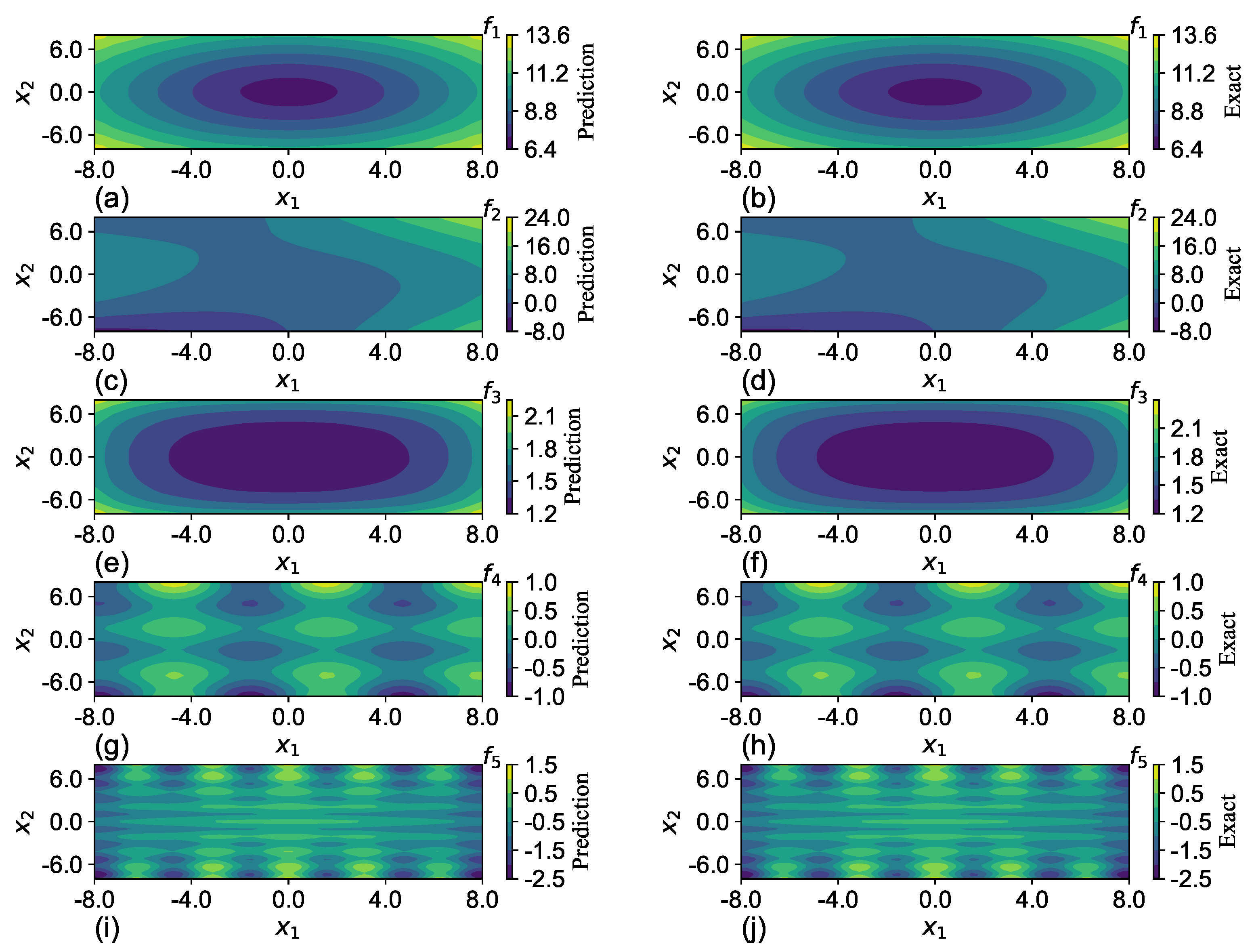
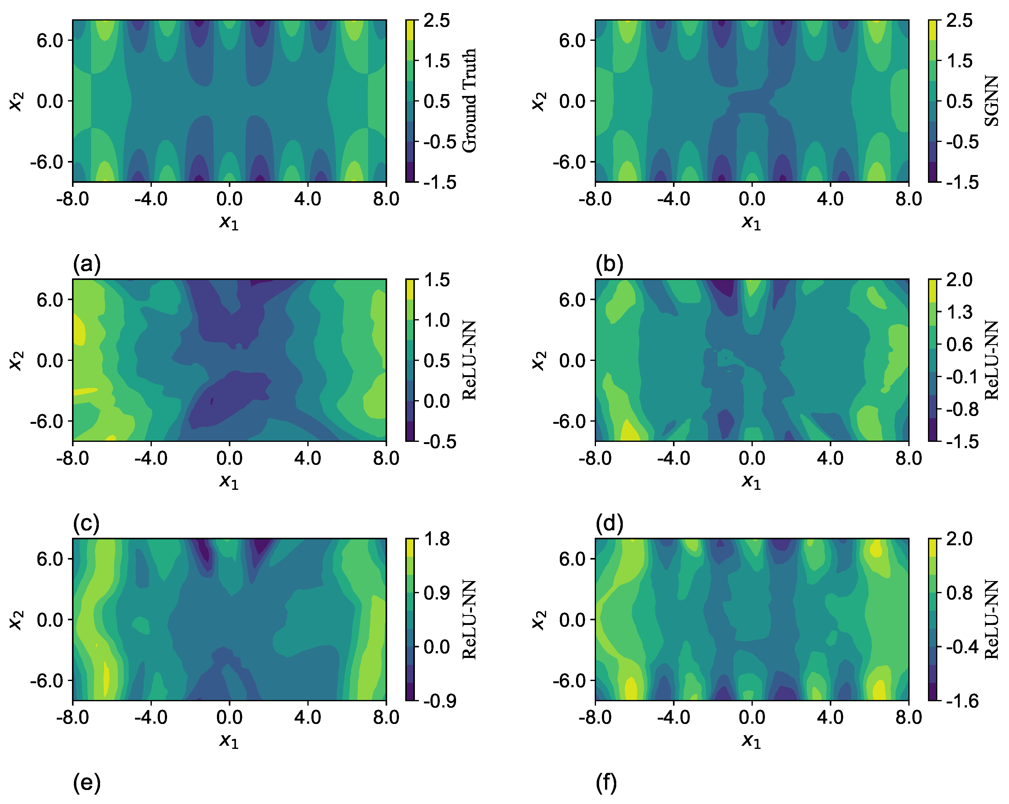
To visualize the differences in the expressiveness between SGNN and ReLU-NN, the predictions of one run in Table 7 are selected and plotted through a cross-sectional cut in the $x_1-x_2$ plane with the other two variables $x_3$ and $x_4$ fixed at zero, as shown in Figure 7. The network configurations are listed in

Table 8. Network configurations of subplots of Figure 7.

Subfigure	Network	Layers	Neurons/Layer
(b)	SGNN	4	40
(c)	ReLU-NN	4	40
(d)	ReLU-NN	7	40
(e)	ReLU-NN	10	40
(f)	ReLU-NN	10	70

. The predictions of SGNN in Figure 7b match well the ground truth in Figure 7a. Despite the minor differences in colors near the origin, their maximum magnitude is less than 0.1. The ReLU-NN with the same structure has a much worse approximation. Although the network gradually captures the main geometric features of $f_5$ by significantly augmenting its structure to 10 layers and 70 neurons per layer, the difference of magnitude can still be as large as 0.5, as shown in Figure 7f.

8. Conclusions

In this paper, we reexamined the structure of GRBFNN in order to make it tractable for problems with high-dimensional input. By using the separable property of Gaussian radial-basis functions, we proposed a new feedforward network called separable-Gaussian-neural-network (SGNN). Different from the traditional MLPs, SGNN splits the input data into multiple columns by dimensions and feeds them into the corresponding layers in sequence. As opposed to GRBFNN, SGNN significantly reduces the number of neurons, trainable variables, and the computational load of forward and backward propagation, leading to the exponential improvement of training efficiency. SGNN can also preserve the dominant subspace of the Hessian matrix of GRBFNN in gradient descent and, therefore, offer comparable minimal loss. Extensive numerical experiments have been carried out, demonstrating that SGNN has superior computational performance over GRBFNN while maintaining a similar level of accuracy. In addition, SGNN is superior to MLPs with ReLU and Sigmoid units when approximating complex functions. However, whether SGNNs can form a dense set of GRBFNN is unclear and is up to further study. Further investigation could also focus on the universal approximability of SGNN and its applications to physics-informed neural networks (PINNs) and reinforcement learning.

References

1. Dyn, N.; Levin, D.; Rirra, S. Numerical Procedures for Surface Fitting of Scattered Data by Radial Functions. SIAM J. Sci. Comput. 1986, 7, 639–659. [Google Scholar] [CrossRef]
2. Duan, Y. A note on the meshless method using radial basis functions. Comput. Math. Appl. 2008, 55, 66–75. [Google Scholar] [CrossRef]
3. Wu, J. Advances in K-Means Clustering: A Data Mining Thinking; Springer: Berlin/Heidelberg, Germany, 2012. [Google Scholar]
4. Akhtar, T.; Shoemaker, C. Multi objective optimization of computationally expensive multi-modal functions with RBF surrogates and multi-rule selection. J. Glob. Optim. 2016, 64, 17–32. [Google Scholar] [CrossRef]
5. Daoud, M.; Mayo, M.; Cunningham, S.J. RBFA: Radial Basis Function Autoencoders. In Proceedings of the 2019 IEEE Congress on Evolutionary Computation (CEC), Wellington, New Zealand, 10–13 June 2019; pp. 2966–2973. [Google Scholar]
6. Yu, H.; Xie, T.; Paszczyñski, S.; Wilamowski, B. Advantages of Radial Basis Function Networks for Dynamic System Design. IEEE Trans. Neural Netw. Learn. Syst. 2011, 58, 5438–5450. [Google Scholar] [CrossRef]
7. Buvanesvari, R.M.; Joseph, K.S. RBFNN: A radial basis function neural network model for detecting and mitigating the cache pollution attacks in named data networking. IET Netw. 2020, 9, 255–261. [Google Scholar] [CrossRef]
8. Du, J.; Zhang, J.; Yang, L.; Li, X.; Guo, L.; Song, L. Mechanism Analysis and Self-Adaptive RBFNN Based Hybrid Soft Sensor Model in Energy Production Process: A Case Study. Sensors 2022, 22, 1333. [Google Scholar] [CrossRef]
9. Tao, K. A Closer Look at the Radial Basis Function (RBF) Networks. In Proceedings of the 27th Asilomar Conference on Signals, Systems and Computers, Pacific Grove, CA, USA, 1–3 November 1993; Volume 1, pp. 401–405. [Google Scholar]
10. Moody, J.; Darken, C.J. Fast Learning in Networks of Locally-Tuned Processing Units. Neural Comput. 1989, 1, 281–294. [Google Scholar] [CrossRef]
11. Broomhead, D.S.; Lowe, D. Multivariable Functional Interpolation and Adaptive Networks. Complex Syst. 1988, 2, 321–355. [Google Scholar]
12. Hornik, K.; Stinchcombe, M.; White, H. Multilayer Feedforward Networks are Universal Approximators. Neural Netw. 1989, 2, 359–366. [Google Scholar] [CrossRef]
13. Park, J.; Sandberg, I.W. Universal Approximation Using Radial-Basis-Function Networks. Neural Comput. 1991, 3, 246–257. [Google Scholar] [CrossRef]
14. Leshno, M.; Lin, V.Y.; Pinkus, A.; Schocken, S. Multilayer Feedforward Networks with a Nonpolynomial Activation Function Can Approximate any Function. Neural Netw. 1993, 6, 861–867. [Google Scholar] [CrossRef]
15. Poggio, T.; Girosi, F. Networks for approximation and learning. Proc. IEEE 1990, 78, 1481–1497. [Google Scholar] [CrossRef]
16. Wettschereck, D.; Dietterich, T.G. Improving the Performance of Radial Basis Function Networks by Learning Center Locations. In Proceedings of the 4th International Conference on Neural Information Processing System, San Francisco, CA, USA, 2–5 December 1991; pp. 1133–1140. [Google Scholar]
17. Platt, J. A Resource-Allocating Network for Function Interpolation. Neural Comput. 1991, 3, 213–225. [Google Scholar] [CrossRef] [PubMed]
18. Chen, S.; Cowan, C.; Grant, P. Orthogonal Least Squares Larning Algorithm for Radial Basis Function Networks. IEEE Trans. Neural Netw. 1991, 2, 302–309. [Google Scholar] [CrossRef]
19. Huang, G.B.; Saratchandran, P.; Sundararajan, N. A Generalized Growing and Pruning RBF (GGAP-RBF) Neural Network for Function Approximation. IEEE Trans. Neural Netw. 2005, 16, 57–67. [Google Scholar] [CrossRef]
20. Carvalho, A.; Brizzotti, M. Combining RBF Networks Trained by Different Clustering Techniques. Neural Process. Lett. 2001, 14, 227–240. [Google Scholar] [CrossRef]
21. Niros, A.; Tsekouras, G. On training radial basis function neural networks using optimal fuzzy clustering. In Proceedings of the 17th Mediterranean Conference on Control and Automation, Thessaloniki, Greece, 24–26 June 2009; pp. 395–400. [Google Scholar]
22. Yao, W.; Chen, X.; Van Tooren, M.; Wei, Y. Euclidean Distance and Second Derivative based Widths Optimization of Radial Basis Function Neural Networks. In Proceedings of the the 2010 International Joint Conference on Neural Networks (IJCNN), Barcelona, Spain, 18–23 July 2010; pp. 1–8. [Google Scholar]
23. Yao, W.; Chen, X.; Zhao, Y.; van Tooren, M. Concurrent Subspace Width Optimization Method for RBF Neural Network Modeling. IEEE Trans. Neural Netw. Learn. Syst. 2012, 23, 247–259. [Google Scholar] [PubMed]
24. Zhang, Y.; Gong, C.; Fang, H.; Su, H.; Li, C.; Da Ronch, A. An efficient space division–based width optimization method for RBF network using fuzzy clustering algorithms. Struct. Multidiscip. Optim. 2019, 60, 461–480. [Google Scholar] [CrossRef]
25. Zheng, S.; Feng, R. A variable projection method for the general radial basis function neural network. Appl. Math. Comput. 2023, 451, 128009. [Google Scholar] [CrossRef]
26. Abadi, M.; Barham, P.; Chen, J.; Chen, Z.; Davis, A.; Dean, J.; Devin, M.; Ghemawat, S.; Irving, G.; Isard, M.; et al. TensorFlow: A system for large-scale machine learning. In Proceedings of the 12th USENIX Symposium on Operating Systems Design and Implementation (OSDI’16), Savannah, GA, USA, 2–4 November 2016; pp. 265–283. [Google Scholar]
27. Paszke, A.; Gross, S.; Massa, F.; Lerer, A.; Bradbury, J.; Chanan, G.; Killeen, T.; Lin, Z.; Gimelshein, N.; Antiga, L.; et al. PyTorch: An Imperative Style, High-Performance Deep Learning Library. In Proceedings of the Neural Information Processing Systems, Vancouver, BC, Canada, 8–14 December 2019; pp. 8024–8035. [Google Scholar]
28. Baydin, A.; Pearlmutter, B.; Radul, A.; Siskind, J. Automatic Differentiation in Machine Learning: A Survey. J. Mach. Learn. Res. 2018, 18, 1–43. [Google Scholar]
29. Sagun, L.; Bottou, L.; LeCun, Y. Eigenvalues of the Hessian in Deep Learning: Singularity and Beyond. arXiv 2017, arXiv:1611.07476. [Google Scholar]
30. Sagun, L.; Evci, U.; Guney, V.U.; Dauphin, Y.; Bottou, L. Empirical Analysis of the Hessian of Over-Parametrized Neural Networks. arXiv 2018, arXiv:1706.04454. [Google Scholar]
31. Gur-Ari, G.; Roberts, D.A.; Dyer, E. Gradient Descent Happens in a Tiny Subspace. arXiv 2018, arXiv:1812.04754. [Google Scholar]
32. Andras, P. Function Approximation Using Combined Unsupervised and Supervised Learning. IEEE Trans. Neural Netw. Learn. Syst. 2014, 25, 495–505. [Google Scholar] [CrossRef]
33. Andras, P. High-Dimensional Function Approximation with Neural Networks for Large Volumes of Data. IEEE Trans. Neural Netw. Learn. Syst. 2018, 29, 500–508. [Google Scholar] [CrossRef]
Figure 1. The general structure of SGNNs. In this paper, the weights of the output layer are in unity. The distinct feature of the SGNN is that input is divided and fed sequentially to hidden layers. Therefore, the depth (layers) of SGNNs is identical to the number of input dimensions. Each neuron in hidden layers is associated with an uni-variate Gaussian function. Each path in feedforward propagation will lead to a chain of multiplications of uni-variate Gaussian functions, equivalent to a d-dimensional Gaussian radial-basis function shown in Equation (4). In other words, each SGNN can be converted to an RGBFNN.
Algorithms 16 00453 g001
Figure 2. Approximating the two-dimensional function f 3 by SGNN. (a) Training history; (b) absolute error; (c) prediction vs. exact value; (d) prediction; and (e) ground truth. Size of the training dataset: 2048.
Algorithms 16 00453 g002
Figure 3. Approximating the two-dimensional f 4 by SGNN. (a) Training history; (b) absolute error; (c) prediction vs. exactness; (d) prediction; and (e) ground truth. Size of training dataset: 2048.
Algorithms 16 00453 g003
Figure 4. Approximating the two-dimensional f 5 by SGNN. (a) Training history; (b) absolute error; (c) prediction vs. exactness; (d) 2D projection of prediction; and (e) 2D projection of ground truth. Size of training dataset: 2048.
Algorithms 16 00453 g004
Figure 5. Prediction vs. exact f 1 f 5 in five dimensions. The plots are generated by projecting the surface to a x 1 x 2 plane with other coordinates fixed to zero. The (left) panel is for prediction; the (right) panel is for the exact value. Size of training dataset: 32,768.
Algorithms 16 00453 g005
Figure 6. Prediction vs. exact of f 6 f 10 in five dimensions. The plots are generated by projecting the surface to the x 1 x 2 plane with other coordinates fixed to zero. (Left) panel: prediction; (right) panel: ground truth. Size of training dataset: 32,768.
Algorithms 16 00453 g006
Figure 7. Approximation of the four-dimensional f 5 using SGNN and ReLU-NNs. The plots are generated by projecting the surface to the x 1 x 2 plane with other coordinates all zero. (a) Ground truth; (b) SGNN; (cf) ReLu-NNs with different network configurations. The layers and neurons per layer of the NNs are listed in Table 8.
Algorithms 16 00453 g007