Abstract
Finding the cluster structure is essential for analyzing self-organized networking structures, such as social networks. In such problems, a wide variety of distance measures can be used. Common clustering methods often require the number of clusters to be explicitly indicated before starting the process of clustering. A preliminary step to clustering is deciding, firstly, whether the data contain any clusters and, secondly, how many clusters the dataset contains. To highlight the internal structure of data, several methods for visual assessment of clustering tendency (VAT family of methods) have been developed. The vast majority of these methods use the Euclidean distance or cosine similarity measure. In our study, we modified the VAT and iVAT algorithms for visual assessment of the clustering tendency with a wide variety of distance measures. We compared the results of our algorithms obtained from both samples from repositories and data from applied problems.
1. Introduction
The identification of the cluster structure in data is useful for discovering the dependencies between the sample objects. Dividing the sample into groups of similar objects simplifies further data processing and decision making, and enables us to apply a separate analysis method to each cluster. A decrease in the number of groups can help us to select the most common patterns in the data. Finding the cluster structure is essential for analyzing self-organized networking structures, such as social networks. In such problems, different measures of distance may be applied.
For evaluating the similarity between objects, we can use the internal and external similarity measures [1]. Measures of internal similarity are based on the proximity of objects within a group and their distance from objects in other groups. Internal similarity measures rely on information obtained only from a dataset. External similarity measures, on the other hand, are based on comparing clustering results with reference results, usually created with the assistance of experts. In this paper, we focus on internal similarity measures. The modern literature provides a wide range of evaluation criteria, such as the Calinski–Harabasz index [2], Dunn index, Davies–Bouldin index [3], silhouette index [4,5], and others.
In the work of Bezdek and Hathaway [6], the authors raised an important question: “Do clusters exist?” Clustering algorithms divide data points into groups according to some criterion so that objects from one group are more similar to each other than to objects from other groups. Clustering algorithms are usually applied in an unsupervised way when vectors of object parameter values or a matrix of differences between objects are used as initial data.
In unsupervised learning, clustering methods form groups of objects, even if the analyzed dataset is a completely random structure. This is one of the most important problems of clustering. Therefore, the first validation task that is recommended to be performed before clustering is to assess the general propensity of the data to cluster (clustering tendency). Before evaluating the performance of clustering, we must make sure that the dataset we are working with tends to cluster and does not contain uniformly distributed points (objects). If the data do not tend to cluster, then the groups identified by any modern clustering algorithm may be meaningless.
The term “clustering tendency” is introduced in [7]. Using it, we can estimate the propensity of the data points to clustering.
Some methods for assessing clustering propensity are discussed in [7,8]. They can be roughly divided into following categories: statistical and visual. In [9], the authors noted that “A clustering index should be an indicator of the degree of non-uniformity of the distribution of the objects. It should be used both as an automatic warning or, better, as a quantitative measure of the quality of the dataset, original or extracted”. The Hopkins clustering index [10,11] has these properties [9]. It is based on the null hypothesis H0: “The points in a dataset are uniformly distributed in multidimensional space”. In a known dataset, X1, …, XN, in a M-dimensional space, B real points are randomly selected and artificial points are added using a distribution with the standard deviation of known data points. For each real and artificial point, the Euclidean distance to the nearest point is determined. The distance between a real point to its nearest point is compared with the distance between an artificial point to nearest real point . If there is a clustering tendency, then [12]. The found minimal distances are summarized for all points and used for the Hopkins clustering index, which is calculated as follows:
where is the Euclidean distance between each of these real points b and their nearest real neighbor k; is the Euclidean distance between these artificial points a and the nearest real point k, . If , then the data points are scattered randomly and it is impossible to extract the cluster structure. If , then the data are homogeneous and there are no clusters, so we can say that all the data make up one big cluster. Approximation of to 1 means that a cluster structure can be identified in the data with a high degree of probability; if , then this is the maximum degree of clustering. To obtain a stable Hopkins clustering index value (mean value), multiple calculations are carried out with new random samples.
In [9,12], the authors presented the modified Hopkins clustering index. This index is calculated as follows:
where is the Euclidean distance between these points n and their real nearest point k, i.e., is computed for all the N points,. If , then it is impossible to distinguish a cluster structure in the data points, if , then this is the maximum degree of clustering [9].
In [9], the minimum spanning tree (MST) clustering index is proposed. The clustering algorithms associated with MST determine whether a point belongs to a cluster based on connectivity. The Prim’s algorithm [13] and the Kruskal algorithm [14] are used to calculate the MST. The MST clustering index is defined as follows [9]:
where dcrit is the critical distance value and d is the tree distance. If then we accept the null hypothesis H0, otherwise, the dataset is not homogeneous. The MST clustering index can be used to find groups, to measure the degree of heterogeneity of data points, and to detect the outliers.
The authors [9] noted that the MST clustering index is sensitive to the empty space outside the multivariate limits of data points. In the case when there are areas of points in the dataset that do not have clear boundaries, the and indexes are unable to determine the clustering tendency. However, all of these methods estimate only tendency to clustering, but not the number of clusters.
For fuzzy clustering approach, there are several methods for estimating cluster validity. For example, Xie-Beni’s separation index (XBI) [15], which expresses the inverse ratio between the total variation and N times the minimum separation of the clusters:
where dmin is the minimum distance of all distances between two clusters, K is the number of clusters, and is calculated as follows:
In [6], the authors presented a tool, named VAT (visual assessment of tendency), for visual assessment of the clustering tendency. At the first step, VAT algorithm reorders the matrix of differences. At the second step, it generates a reordered dissimilarity image (RDI)—a cluster heat map. In a cluster heat map, dark areas located on the main diagonal enable us to determine the possible number of groups [16]. The VAT can be used for any numerical datasets. The VAT algorithm is similar to Prim’s algorithm [13] for determining an MST of a weighted graph. The authors of the VAT algorithm noted the two following differences. Firstly, the VAT algorithm does not require their MST representation, only the order in which vertices are added as the graph grows is important. Secondly, in the VAT algorithm, the choice of the initial vertex depends on the maximum weight of the edge. In cases of a complex data structure, the efficiency of the VAT algorithm decreases quickly. However, VAT works well for datasets with dimension N ≤ 500. For datasets with higher dimensions, the time complexity of the algorithm (O(N2)) increases.
In [17], the authors proposed an improved VAT (iVAT) algorithm. The iVAT images more clearly showed the number of groups, as well as their sizes. As the authors assure in [17]: “Based on the iVAT image, the cluster structure in the data can be reliably estimated by visual inspection”. In addition, the authors proposed automated VAT (aVAT). The article [18] describes a method that handles asymmetric dissimilarity data (asymmetric iVAT (asiVAT)). In [19], the authors presented an approach for finding the number of groups by traversing the MST backwards by cutting (k – 1) the largest edge in the MST.
VAT and iVAT have two restrictions:
- 1)
- RDI may not be representative if the cluster structure in the data points is complex.
- 2)
- The quality of the RDI in VAT is significantly degraded due to the presence of outliers.
The revised visual assessment of cluster tendency (reVAT) algorithm [20], using a quasi-ordering of the N points, reduces the time complexity to O(n). The reVAT does not require reordering the matrix of differences. The reVAT plots a set of c profile graphs of specific rows of an ordered difference matrix. An ensemble of a set of c profile graphs is used to visually determine the number of groups [20]. However, when the number of clusters is large and there are areas of points that do not have clear boundaries, a visual assessment of the number of clusters is difficult with the use of reVAT.
Research [21] has presented a visual assessment of the clustering trend for large and relational datasets (bigVAT). This method uses the quasi-ordering from reVAT and builds an image similar to that built by VAT. The bigVAT solves the problems of the VAT and reVAT methods [20]. However, the image it builds may not be as visual as the image ordered by VAT.
In [22], the authors presented the scalable VAT (sVAT) algorithm. To create an image, the sVAT algorithm generates a representative sample containing a structure of clusters similar to that of the original dataset. For this sample, sVAT generates a VAT-ordered image considering the following parameters: an overpriced grade of the actual number of clusters (k) and the size of representative sample (n) from the full set of N points. The sample is formed as follows: a set of k distinguished points is selected, then additional data are added next to each of the k objects. In addition, [23] described the method for visual assessment of the clustering tendency for rectangular matrices of differences (coVAT).
The cluster count extraction (CCE) algorithm [24] creates a visual image using the VAT algorithm. This algorithm further processes the image to improve it for automatic verification, and extracts the number of clusters from the improved image. The article [25] demonstrates the dark block extraction (DBE) method. This method generates an RDI (VAT image) and then segments the desired areas into RDI and converts the filtered image to a distance transform image. The transformed image is superimposed on the RDI diagonal and the potential number of groups is determined. The CCE and DBE algorithms automatically determine the number of groups in unlabeled data points.
Paper [26] presents the CLODD (cluster in ordered difference data) method. In this algorithm, to identify potential clusters, an objective function is determined that combines contrast and edginess measures and is optimized using particle swarm optimization (PSO) [27]. With the help of the objective function, the block structure is recognized in the reordered dissimilarity matrix. The CLODD algorithm is used both to search for clusters in unlabeled data and to represent the validity index of these clusters.
The effectiveness of the considered methods based on the SDS largely depends on the quality of the SDS images. SDS is effective only for defining compact clearly marked groups. However, there are datasets that have a very complex structure of clusters.
In [28], the authors presented a novel silhouette-based clustering propensity score (SACT) algorithm for determining the potential number of clusters and their centroids in applications for hyperspectral image analysis. The SACT algorithm was inspired by the VAT algorithm. The SACT algorithm builds a weighted matrix and a weighted graph using the Euclidean distance measure, then, a minimum spanning tree is constructed using Prim’s algorithm. The original minimum spanning tree is then hashed into branches corresponding to data clusters. Finally, the number of potential clusters is determined using the silhouette index.
Clustering datasets with different cluster density is a difficult problem. The VAT and iVAT algorithms use the difference between intra-cluster and inter-cluster distances to discover the data structure. These algorithms do not work well for data points consisting of groups with different levels of density. In [29], the authors introduced the locally scaled VAT (LS-VAT) algorithm and locally scaled iVAT (LS-iVAT) algorithm. In the LS-VAT algorithm, before generating the MST, the distance matrix is converted into an adjacency matrix using local scaling [30]. The algorithm builds a similarity graph for a dataset; for this, instead of connecting the data point that has the smallest distance from the current tree, it connects the data point that has the highest adjacency to the existing tree. In case a set of points with different inter-cluster densities is used, the LS-iVAT algorithm must be used to provide higher quality iVAT images. LS-VAT and LS-iVAT outperform algorithms [6,16,31,32] in terms of clustering quality.
In [33], the authors presented a semi-supervised constraint-based approach for the iVAT (coniVAT) algorithm. To improve VAT/iVAT for complex data points, coniVAT uses partial background knowledge in the form of constraints. ConiVAT uses the input constraints to learn a basic similarity measure, builds a minimum transitive matrix of differences, and then applies VAT to it.
For big datasets, algorithms ClusiVAT [34] and S-MVCS-VAT [35] were developed. In [36], the spectral technique was applied to ClusiVAT and S-MVCS-VAT algorithms. An algorithm based on VAT for streaming data processing was presented in [37].
Kumar and Bezdek [15] presented a detailed and systematic review of a variety of VAT and iVAT algorithms and models. This article describes 25 algorithms.
Thus, VAT/iVAT algorithms are methods for visually extracting some information about the structure of clusters from the initial dataset before applying any clustering algorithm. They do not change the initial dataset, but rearrange the objects in such a way as to emphasize the possible structure of the cluster.
Most of the considered algorithms use the Euclidean distance measure. However, it is known that, depending on the shape of the clusters, different distance measures are better suited for different datasets. Despite the fact that there are many distance measures (similarity measures) in the literature [16,18,38], it is quite difficult to choose the right one for a specific dataset. The choice of the distance measure that is most appropriate in each specific case allows obtaining clearer RDIs and, accordingly, obtaining a more valid result of pre-clustering. In our work, we propose a modification of VAT and iVAT algorithms convenient for using other distance measures than Euclidean. We discover the behavior of modified algorithms on the applied dataset and datasets from the repositories.
2. Materials and Methods
Consider a set of points where each point is represented as a characteristic vector of dimension p, xi ∈ Rp, X = {x1,.., xn} ∈ Rp. The second way to represent the points is the dissimilarity matrix D = [dij] (1), of n × n dimension, where dij is difference between the points I and j, calculated using a distance measure.
The dissimilarity matrix has several properties:
- Symmetry about the diagonal. The dissimilarity matrix is a square symmetrical n × n matrix with dij element equal to the value of a chosen measure of distinction between the ith and jth objects dij = dji.
- The distance values in the matrix are always non-negative dij ≥ 0.
- Identity of indiscernibles. In the matrix, the distinction between an object and itself is set to zero (dii is diagonal element, where dii = 0).
- The triangle inequality takes the form dij + djk ≥ dik ∀ i,j,k.
The quality of the cluster solution also depends on the chosen distance measure. In this work, we used some distance measures (the Euclidean distance, the squared Euclidean distance, the Manhattan distance, the Chebyshev distance) based on the Minkowski function (lp-norm) [39,40,41]:
where x and y are input vectors of dimension M. For parameter p, the following statement is true (proof): for p ≥ 1 and p = ∞, the distance is a metric; for p < 1, the distance is not a metric.
For p = 2, the function takes the form of Euclidean distance (l2 norm):
The Euclidean distance is the most understandable and interpretable measure of the difference between points represented by feature vectors in multidimensional space. Therefore, the Euclidean distance and squared Euclidean distance are widely used for data analysis. The squared Euclidean distance is defined as:
We also used the standardized Euclidean distance, calculated as follows:
where si is standard deviation of the ith characteristic of the input data vectors.
For p = 1, we obtained the Manhattan distance (l1 -norm), which is the second most popular distance:
For , the function calculates the Chebyshev distance [42], also called the chessboard distance:
Most modern papers are devoted to problems that use the Euclidean or Manhattan distances.
There are other ways to calculate distances that do not depend on the parameter p and are not determined by the Minkowski function. For example, we used the Mahalanobis distance [43], the correlation-based distance (the correlation distance) [44], the cosine similarity [45], the Bray–Curtis dissimilarity [46], the Canberra distance [42].
Mahalanobis distance is defined as
where C is the covariance matrix calculated as
where μ is the mean value.
The correlation distance is defined by:
where and are the means of the elements of x and y, respectively, and means norm, which is, by default, a second-order (Euclidean) norm.
The measure of similarity can be estimated through the cosine of the angle between two vectors:
where means norm, which is, by default, a second order (Euclidean) norm.
Bray–Curtis dissimilarity [46] is defined by:
Canberra distance [42] is given as follows:
VAT [6,16] and iVAT algorithms [47] are tools for visual assessment of the tendency to clustering of a set of points by reordering the dissimilarity matrix such that possible clusters appear as dark boxes diagonally in the cluster heat map. This cluster heat map can be used to visually estimate the number of clusters in a dataset [33]. VAT reordering is related with clusters created using single linker hierarchical clustering (SL), which makes it possible to extract SL-aligned groups from images of VAT (iVAT) [48].
The VAT algorithm is presented below (Algorithm 1) [6,15].
| Algorithm 1. Visual assessment of the clustering tendency (VAT). |
|
In [16], the authors proposed an improved VAT (iVAT). This algorithm transforms the dissimilarity matrix with the idea, which is the following: when two distant objects are connected by a chain of other objects closely located, to reflect this connection, the distance dij between them has to be reduced. According to this correction, two objects, if connected by a set of successive objects forming dense regions, should be considered coming from one cluster [15]. The iVAT algorithm is presented in Algorithm 2 [15,16].
| Algorithm 2. Improved visual assessment of the clustering tendency (iVAT). |
|
In this research, we modified the VAT and iVAT algorithms in such a way to be able to calculate many possible distance measures besides the Euclidean (DVAT or DiVAT, see Algorithm 3).
| Algorithm 3. DVAT (DiVAT) algorithm. |
|
3. Results of Computational Experiment
Computational experiment results of the visual assessment of the clustering tendency based on the VAT and iVAT algorithms with variations of distance measures are presented. The considered distance measures included: Euclidean distance, squared Euclidean distance, standardized Euclidean distance, Manhattan distance, Mahalanobis distance, Bray–Curtis dissimilarity, Canberra distance, Chebyshev distance, distance correlation, cosine similarity.
For the experiments, we used synthetic (artificial) datasets (with cluster labels) [49], as well as from samples of industrial products [50,51] and from a set of some taxation characteristics of forest stands [52]:
- a)
- Long2 is an artificial dataset that contains the collection of two clusters (1000 data points, 2 dimensions) (Figure 1a).
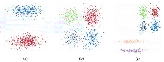 Figure 1. (a) Synthetic dataset Long2; (b) synthetic dataset Sizes1; (c) synthetic dataset Longsquare.
 - b)
- Sizes1 is an artificial dataset contains the collection of four clusters (1000 data points, 2 dimensions) (Figure 1b).
- c)
- Longsquare is an artificial dataset contains the collection of six clusters (1000 data points, 2 dimensions) (Figure 1c).
- d)
- Microchips are two sets of results of test effects on electrical and radio products for monitoring the current–voltage characteristics of input and output circuits of microcircuits: Microchips 140UD25AS1VK (46 data points, 9 dimensions, 2 clusters) and 1526IE10_002 (3987 data points, 67 dimensions, 4 clusters) [50,51]. For microchip 1526IE10_002, we used the following batch combinations: mixed lots from four (62 parameters), three (41 parameters), and two batches (41 parameters).
- e)
- Siberian Forest Compartments Dataset [52] is a set of some taxation characteristics of forest stands, on which outbreaks of mass reproduction of the Siberian silkworms were recorded at a certain time (15,523 data points, 150 dimensions). The Siberian Forest Compartments Dataset contains three forestry strands: Irbey forestry (2330 data points), Chunsky forestry (3271 data points), and Lower Yenisei forestry (3619 data points).
In our experiments, the following test system was used: Intel (R) Core (TM) i5-8250U CPU, 16 GB RAM, while Python was also used to implement the algorithms.
3.1. Synthetic Datasets
The computational experiment showed that the resulting iVAT images more clearly showed the number of clusters than the resulting VAT images (Appendix A, Figure A1) for Long2. In addition, it can be noted that the Mahalanobis distance and squared Euclidean distance had an advantage over the other distances (Appendix A, Figure A1). The VAT and iVAT algorithms with Canberra distance did not cope with the task. The VAT and iVAT images showed four clusters. The VAT image with Bray–Curtis dissimilarity and cosine similarity showed no clusters (Appendix A, Figure A1).
For the Sizes1 dataset, the computational experiment showed that the resulting iVAT images more clearly showed the number of clusters than the resulting VAT images (Appendix A, Figure A2). In addition, the Canberra distance and cosine similarity had an advantage over the other distances (Appendix A, Figure A2). The VAT and iVAT algorithms with distance correlation did not cope with the task. The VAT and iVAT images showed two clusters. The VAT image with Bray–Curtis dissimilarity showed no clusters (Appendix A, Figure A2).
For Longsquare, the computational experiment showed that the resulting iVAT images more clearly showed the number of clusters than the resulting VAT images (Appendix A, Figure A3). In addition, the Mahalanobis distance and squared Euclidean distance had an advantage over the other distances (Appendix A, Figure A3). The VAT and iVAT algorithms with Bray–Curtis dissimilarity, distance correlation, Canberra distance, and cosine similarity did not cope with the task. The VAT and iVAT images with distance correlation and iVAT images with cosine similarity showed two clusters, while the VAT image with Bray–Curtis dissimilarity showed no clusters (Appendix A, Figure A3).
3.2. Microchips Datasets
For Microchips 140UD25AS1VK, the computational experiment showed that the resulting iVAT images more clearly showed the number of clusters than the resulting VAT images. The VAT and iVAT algorithms with Mahalanobis distance did not cope with the task. The VAT and iVAT images with Mahalanobis distance did not show actual clusters. The iVAT image with distance correlation and cosine similarity showed better performance (Appendix A, Figure A4).
For Microchips 1526IE10_002, four-batch mixed lot, the computational experiment showed that the VAT and iVAT algorithms with Mahalanobis distance, Chebyshev distance, and iVAT with squared Euclidean distance did not cope with the task. The VAT and iVAT images with Mahalanobis distance and the iVAT with squared Euclidean distance showed no clusters (Appendix A, Figure A5).
For Microchips 1526IE10_002, three-batch mixed lot, the computational experiment showed that the resulting iVAT images more clearly showed the number of clusters than the resulting VAT images (Appendix A, Figure A6). The cosine similarity and squared Euclidean distance had an advantage over the other distances (Appendix A, Figure A6). The VAT and iVAT algorithms with Mahalanobis distance and Chebyshev distance did not cope with the task. The VAT and iVAT images with Mahalanobis showed no clusters (Appendix A, Figure A6).
For Microchips 1526IE10_002, two-batch mixed lot, the computational experiment showed that the resulting iVAT images more clearly showed the number of clusters than the resulting VAT images (Appendix A, Figure A7). The VAT and iVAT algorithms with Mahalanobis distance and Chebyshev distance did not cope with the task. The VAT and iVAT images with Mahalanobis showed no clusters (Appendix A, Figure A7).
3.3. Siberian Forest Compartments Datasets
For Chunsky forestry, the computational experiment showed that the resulting iVAT images more clearly showed the number of clusters than the resulting VAT images. However, the Euclidean distance and squared Euclidean distance had an advantage over the other distances (Appendix A, Figure A8).
For Irbey forestry, the computational experiment showed that the resulting iVAT images more clearly showed the number of clusters than the resulting VAT images. The Canberra distance, distance correlation, and cosine similarity had an advantage over the other distances (Appendix A, Figure A9).
For Lower Yenisei forestry, computational experiment showed that the resulting iVAT images more clearly showed the number of clusters than the resulting VAT images (Appendix A, Figure A10).
4. Discussion
Before applying any clustering method, it is important to evaluate cluster validity, i.e., to assess whether the datasets contain meaningful clusters. If clusters exist, then the assessment of the cluster tendency is a good tool to get prior knowledge of the number of clusters in problems such as k-means, where calculating the k value is a challenge.
Despite the fact that there are many similarity measures that have been considered in the literature, it is quite difficult to choose the right one for a specific dataset. Due to the multidimensionality of the data, the cluster structure is not visible explicitly, so the choice of the most suitable distance measure makes it possible to clearly identify this structure. In this research, we modified the VAT and iVAT algorithms in such a way to be able to calculate many possible distance measures besides the Euclidean. The computational experiments showed that using different similarity measures in VAT and iVAT algorithms allows the expert to more confidently estimate the clustering tendency of the dataset.
The computational experiments showed that cluster heat maps produced by the iVAT algorithm in all cases had higher contrast than produced by the VAT algorithm and, hence, were more clear for interpretation.
Our studies have shown that distance measure significantly affects the visual tendency of clustering. In most cases, the best results were obtained with squared Euclidean distance unlike Euclidean distance, which is usually used by default in the VAT family of algorithms.
Author Contributions
Conceptualization, G.S. and E.T.; methodology, G.S.; software, N.R.; validation, G.S., N.R. and E.T.; formal analysis, N.R.; investigation, N.R.; resources, L.K.; data curation, L.K.; writing—original draft preparation, G.S. and E.T.; writing—review and editing, E.T. and L.K.; visualization, N.R.; supervision, G.S.; project administration, L.K.; funding acquisition, L.K. All authors have read and agreed to the published version of the manuscript.
Funding
This research was funded by the Ministry of Science and Higher Education of the Russian Federation, project no. FEFE-2020-0013.
Conflicts of Interest
The authors declare no conflict of interest.
Appendix A

Figure A1.
Long2. Cluster heat map.

Figure A2.
Sizes1. Cluster heat map.

Figure A3.
Longsquare. Cluster heat map.

Figure A4.
140UD25AS1VK. Cluster heat map.

Figure A5.
Microchips 1526IE10_002, four-batch mixed lot. Cluster heat map.

Figure A6.
Microchips 1526IE10_002, three-batch mixed lot. Cluster heat map.

Figure A7.
Microchips 1526IE10_002, two-batch mixed lot. Cluster heat map.

Figure A8.
Chunsky forestry. Cluster heat map.

Figure A9.
Irbey forestry. Cluster heat map.

Figure A10.
Lower Yenisei forestry. Cluster heat map.
References
- Amigó, E.; Gonzalo, J.; Artiles, J.; Verdejo, M.F. A comparison of extrinsic clustering evaluation metrics based on formal constraints. Inf. Retr. 2009, 12, 613. [Google Scholar] [CrossRef]
- Calinski, R.B.; Harabasz, J. A dendrite method for cluster analysis. Commun. Stat. 1974, 3, 1–27. [Google Scholar]
- Davies, D.L.; Bouldin, D.W. A cluster separation measure. IEEE Trans. Pattern Anal. Mach. Intell. 1979, 1, 224–227. [Google Scholar] [CrossRef]
- Kaufman, L.; Rousseeuw, P.J. Finding Groups in Data: An Introduction to Cluster Analysis; Wiley: New York, NY, USA, 1990; p. 368. [Google Scholar]
- Rousseeuw, P. Silhouettes: A graphical aid to the interpretation and validation of cluster analysis. J. Comput. Appl. Math. 1987, 20, 53–65. [Google Scholar] [CrossRef]
- Bezdek, C.; Hathaway, R.J. Vat: A tool for visual assessment of (cluster) tendency. In Proceedings of the IJCNN, Honolulu, HI, USA, 12–17 May 2002; pp. 2225–2230. [Google Scholar]
- Jain, A.K.; Dubes, R.C. Algorithms for Clustering Data; Prentice Hall College Div: Hoboken, NJ, USA, 1988. [Google Scholar]
- Everitt, B. Graphical Techniques for Multivariate Data; North-Holland Press: New York, NY, USA, 1978. [Google Scholar]
- Forina, M.; Lanteri, S.; Díez, I. New index for clustering tendency. Anal. Chim. Acta 2001, 446, 59–70. [Google Scholar] [CrossRef]
- Hopkins, B.; Skellam, J.G. A New Method for determining the Type of Distribution of Plant Individuals. Ann. Bot. 1954, 18, 213–227. [Google Scholar] [CrossRef]
- Lawson, R.G.; Jurs, P.J. Cluster analysis of acrylates to guide sampling for toxicity testing. J. Chem. Inf. Comput. Sci. 1990, 30, 137–144. [Google Scholar] [CrossRef]
- Fernández Pierna, J.A.; Massart, D.L. Improved algorithm for clustering tendency. Anal. Chim. Acta 2000, 408, 13–20. [Google Scholar] [CrossRef]
- Prim, R.C. Shortest Connection Networks and some Generalizations. Bell Syst. Tech. J. 1957, 36, 1389–1401. [Google Scholar] [CrossRef]
- Kruskal, J.B. On the Shortest Spanning Subtree of a Graph and the Traveling Salesman Problem. Proc. Am. Math. Soc. 1956, 7, 48–50. [Google Scholar] [CrossRef]
- Xie, X.L.; Beni, G. A Validity Measure for Fuzzy Clustering. IEEE Trans. Pattern Anal. Mach. Intel. 1991, 13, 841–847. [Google Scholar] [CrossRef]
- Kumar, D.; Bezdek, J.C. Visual approaches for exploratory data analysis: A survey of the visual assessment of clustering tendency (VAT) family of algorithms. IEEE Trans. Syst. Man Cybern. 2020, 6, 10–48. [Google Scholar] [CrossRef]
- Wang, L.; Nguyen, U.T.; Bezdek, J.C.; Leckie, C.A.; Ramamohanarao, K. iVAT and aVAT: Enhanced visual analysis for cluster tendency assessment. In Proceedings of the Pacific-Asia Conference on Knowledge Discovery and Data Mining, Hyderabad, India, 21–24 June 2010; Springer: Berlin/Heidelberg, Germany, 2010; pp. 16–27. [Google Scholar]
- Havens, T.C.; Bezdek, J.C.; Leckie, C.; Palaniswami, M. Extension of iVAT to asymmetric matrices. In Proceedings of the Fuzzy Systems (FUZZ), 2013 IEEE International Conference, Hyderabad, India, 7–10 July 2013; pp. 1–6. [Google Scholar]
- Zhong, C.; Yue, X.; Lei, J. Visual hierarchical cluster structure: A refined coassociation matrix based visual assessment of cluster tendency. Pattern Recognit. Lett. 2015, 59, 48–55. [Google Scholar] [CrossRef]
- Huband, J.M.; Bezdek, J.C.; Hathaway, R.J. Revised visual assessment of (cluster) tendency (reVAT). In Proceedings of the North American Fuzzy Information Processing Society (NAFIPS), Banff, AB, Canada, 27–30 June 2004; pp. 101–104. [Google Scholar]
- Huband, J.; Bezdek, J.; Hathaway, R. BigVAT: Visual assessment of cluster tendency for large data sets. Pattern Recognit. 2005, 38, 1875–1886. [Google Scholar] [CrossRef]
- Hathaway, R.; Bezdek, J.C.; Huband, J. Scalable visual assessment of cluster tendency for large data sets. Pattern Recognit. 2006, 39, 1315–1324. [Google Scholar] [CrossRef]
- Bezdek, J.C.; Hathaway, R.; Huband, J. Visual assessment of clustering tendency for rectangular dissimilarity matrices. IEEE Trans. Fuzzy Syst. 2007, 15, 890–903. [Google Scholar] [CrossRef]
- Sledge, I.; Huband, J.; Bezdek, J.C. (Automatic) cluster count extraction from unlabeled datasets. In Proceedings of the Joint International Conference on Natural Computation and International Conference on Fuzzy Systems and Knowledge Discovery, Jinan, China, 1820 October 2008; Volume 1, pp. 3–13. [Google Scholar]
- Wang, L.; Leckie, C.; Kotagiri, R.; Bezdek, J. Automatically determining the number of clusters in unlabeled data sets. IEEE Trans. Knowl. Data Eng. 2009, 21, 335–350. [Google Scholar] [CrossRef]
- Havens, T.C.; Bezdek, J.C.; Keller, J.M.; Popescu, M. Clustering in ordered dissimilarity data. Int. J. Intell. Syst. 2009, 24, 504–528. [Google Scholar] [CrossRef]
- Clerc, M.; Kennedy, J. The particle swarm—Explosion, stability, and convergence in a multi-dimensional complex space. IEEE Trans. Evolut. Comput. 2002, 6, 58–73. [Google Scholar] [CrossRef]
- Pham, N.V.; Pham, L.T.; Nguyen, T.D.; Ngo, L.T. A new cluster tendency assessment method for fuzzy co-clustering in hyperspectral image analysis. Neurocomputing 2018, 307, 213–226. [Google Scholar] [CrossRef]
- Kumar, D.; Bezdek, J.C. Clustering tendency assessment for datasets having inter-cluster density variations. In Proceedings of the 2020 International Conference on Signal Processing and Communications (SPCOM), Bangalore, India, 19–24 July 2020; pp. 1–5. [Google Scholar] [CrossRef]
- Zelnik-manor, L.; Perona, P. Self-tuning spectral clustering. In Advances in Neural Information Processing Systems; MIT Press: Cambridge, MA, USA, 2004; Volume 17, pp. 1601–1608. [Google Scholar]
- Perona, P.; Freeman, W. A factorization approach to grouping. In Proceedings of the Computer Vision—ECCV’98, Freiburg, Germany, 2–6 June 1998; Springer: Berlin/Heidelberg, Germany, 1998; Volume 1406, pp. 655–670. [Google Scholar]
- Campello, R.J.G.B.; Moulavi, D.; Sander, J. Density-based clustering based on hierarchical density estimates. In Advances in Knowledge Discovery and Data Mining; Springer: Berlin/Heidelberg, Germany, 2013; pp. 160–172. [Google Scholar]
- Rathore, P.; Bezdek, J.C.; Santi, P.; Ratti, C. ConiVAT: Cluster Tendency Assessment and Clustering with Partial Background Knowledge. arXiv 2020, arXiv:2008.09570. [Google Scholar]
- Rathore, P.; Bezdek, J.C.; Palaniswami, M. Fast Cluster Tendency Assessment for Big, High-Dimensional Data. In Fuzzy Approaches for Soft Computing and Approximate Reasoning: Theories and Applications; Lesot, M.J., Marsala, C., Eds.; Studies in Fuzziness and Soft Computing; Springer: Cham, Switzerland, 2021; Volume 394. [Google Scholar]
- Basha, M.S.; Mouleeswaran, S.K.; Prasad, K.R. Sampling-based visual assessment computing techniques for an efficient social data clustering. J. Supercomput. 2021, 8, 8013–8037. [Google Scholar] [CrossRef]
- Prasad, K.R.; Kamatam, G.R.; Myneni, M.B.; Reddy, N.R. A novel data visualization method for the effective assessment of cluster tendency through the dark blocks image pattern analysis. Microprocess. Microsyst. 2022, 93, 104625. [Google Scholar] [CrossRef]
- Datta, S.; Karmakar, C.; Rathore, P.; Palaniswami, M. Scalable Cluster Tendency Assessment for Streaming Activity Data using Recurring Shapelets. In Proceedings of the 44th Annual International Conference of the IEEE Engineering in Medicine & Biology Society (EMBC), Glasgow, UK, 11–15 July 2022; pp. 1036–1040. [Google Scholar] [CrossRef]
- Wang, L.; Geng, X.; Bezdek, J.; Leckie, C.; Kotagiri, R. Enhanced visual analysis for cluster tendency assessment and data partitioning. IEEE Trans. Knowl. Data Eng. 2010, 22, 1401–1414. [Google Scholar] [CrossRef]
- Shirkhorshidi, S.; Aghabozorgi, S.; Wah, T. A Comparison Study on Similarity and Dissimilarity Measures in Clustering Continuous Data. PLoS ONE 2015, 10, e0144059. [Google Scholar] [CrossRef]
- Alfeilat, H.; Hassanat, A.; Lasassmeh, O.; Tarawneh, A.; Alhasanat, M.; Salman, H.; Prasath, V. Effects of Distance Measure Choice on K-Nearest Neighbor Classifier Performance: A Review. Big Data 2019, 7, 221–248. [Google Scholar] [CrossRef]
- Weller-Fahy, D.J.; Borghetti, B.J.; Sodemann, A.A. A Survey of Distance and Similarity Measures Used Within Network Intrusion Anomaly Detection. IEEE Commun. Surv. Tutor. 2015, 17, 70–91. [Google Scholar] [CrossRef]
- Canberra Distance. Available online: https://academic.oup.com/comjnl/article/9/1/60/348137?login=false (accessed on 14 October 2022).
- McLachlan, G. Mahalanobis Distance. Resonance 1999, 4, 20–26. [Google Scholar] [CrossRef]
- Distance Correlation. Available online: https://arxiv.org/abs/0803.4101 (accessed on 14 October 2022).
- Han, J.; Kamber, M.; Pei, J. Data mining: Concepts and Techniques; Morgan Kaufmann: Burlington, MA, USA, 2012. [Google Scholar]
- Bray–Curtis Dissimilarity. Available online: https://esajournals.onlinelibrary.wiley.com/doi/10.2307/1942268 (accessed on 14 October 2022).
- Havens, C.; Bezdek, J.C. An efficient formulation of the improved visual assessment of cluster tendency (iVAT) algorithm. IEEE Trans. Knowl. Data Eng. 2012, 24, 813–822. [Google Scholar] [CrossRef]
- Havens, T.C.; Bezdek, J.C.; Keller, J.M.; Popescu, M.; Huband, J.M. Is VAT really single linkage in disguise? Ann. Math. Artif. Intell. 2009, 55, 237. [Google Scholar] [CrossRef]
- Artificial Clustering Datasets. Available online: https://github.com/milaan9/Clustering-Datasets (accessed on 14 October 2022).
- Shkaberina, G.S.; Orlov, V.I.; Tovbis, E.M.; Kazakovtsev, L.A. On the Optimization Models for Automatic Grouping of Industrial Products by Homogeneous Production Batches. Commun. Comput. Inf. Sci. 2020, 1275, 421–436. [Google Scholar]
- Kazakovtsev, L.A.; Antamoshkin, A.N.; Masich, I.S. Fast deterministic algorithm for EEE components classification. IOP Conf. Ser. Mater. Sci. Eng. 2015, 94, 012015. [Google Scholar] [CrossRef]
- Rezova, N.; Kazakovtsev, L.; Shkaberina, G.; Demidko, D.; Goroshko, A. Data pre-processing for ecosystem behaviour analysis. In Proceedings of the 2022 IEEE International Conference on Information Technologies, Varna, Bulgaria, 15–16 September 2022. in press. [Google Scholar]
Disclaimer/Publisher’s Note: The statements, opinions and data contained in all publications are solely those of the individual author(s) and contributor(s) and not of MDPI and/or the editor(s). MDPI and/or the editor(s) disclaim responsibility for any injury to people or property resulting from any ideas, methods, instructions or products referred to in the content. |
© 2022 by the authors. Licensee MDPI, Basel, Switzerland. This article is an open access article distributed under the terms and conditions of the Creative Commons Attribution (CC BY) license (https://creativecommons.org/licenses/by/4.0/).