Solving the Parallel Drone Scheduling Traveling Salesman Problem via Constraint Programming

Abstract

Drones are currently seen as a viable way of improving the distribution of parcels in urban and rural environments, while working in coordination with traditional vehicles, such as trucks. In this paper, we consider the parallel drone scheduling traveling salesman problem, where a set of customers requiring a delivery is split between a truck and a fleet of drones, with the aim of minimizing the total time required to serve all the customers. We propose a constraint programming model for the problem, discuss its implementation and present the results of an experimental program on the instances previously cited in the literature to validate exact and heuristic algorithms. We were able to decrease the cost (the time required to serve customers) for some of the instances and, for the first time, to provide a demonstrated optimal solution for all the instances considered. These results show that constraint programming can be a very effective tool for attacking optimization problems with traveling salesman components, such as the one discussed.

1. Introduction

E-commerce has experienced a boom in recent decades and, according to statistics provided by Statista (https://www.statista.com/statistics/379046/worldwide-retail-e-commerce-sales/, accessed on 8 January 2023), an enormous increase in e-commerce sales is occurring worldwide. One consequence is a huge increase in home-delivered parcels, which can be readily observed in our own cities. It has been reported [1] that many e-commerce and parcel delivery companies are offering ever faster delivery, such as same-day and instant delivery. The report suggests that 20 to 25% of consumers are willing to pay more to receive their parcel on the same day, and 2% would want instant delivery. Companies may be able to offer this kind of delivery through application of cutting-edge technology, such as the use of different types of vehicles, including aerial drones. In [2], the authors forecast that autonomous vehicles, including drones, will deliver about 80% of all parcels in the coming decades. Among the different aspects of the use of aerial drones for last mile deliveries, we focus on operational planning, aiming at optimized delivery strategies. There are several advantages associated with the use of aerial drones: they do not need to follow the road network and can fly in (almost) straight lines, and they are not affected by traffic congestion. These properties also have an important positive impact on sustainability, making these innovative solutions of interest to companies (through reduction in costs), to customers (through more efficient delivery services) and for the whole of society (through more sustainable logistics).

The seminal work of [3] pioneered a new routing optimization problem in which a truck and a drone collaborate to make deliveries. From an operational research perspective, the authors present two new prototypical variants developed from the traditional traveling salesman problem (TSP) called flying sidekick TSP (FSTSP) and parallel drone scheduling TSP (PDSTSP). In both cases a truck and drones collaborate to deliver parcels, the difference being that, in the former, model drones can be launched and collected from the truck during its tour, while, in the latter, the drones are operated directly from the central depot, while the truck executes a traditional delivery tour. In the remainder of the paper, we will focus on the second problem, addressing the interested reader to [4] for full details and some solution strategies for the FSTSP.

More specifically, in the PDSTSP, there is a truck that can leave the depot, serve a set of customers, and return to the depot, and a set of drones, each of which can leave the depot, serve a customer, and return to the depot before serving other customers. Not all the customers can be served by the drones, either due to their location or the characteristics of their parcel. The objective of the approach is to minimize the time needed to serve all the customers and to get the last vehicle back to the depot.

A first mixed-integer linear programming (MILP) model for the PDSTSP and some heuristic methods [5,6] are proposed in [3]. A more refined model, and the first metaheuristic method, based on a two-step strategy embedding a dynamic programming-based component, are discussed in [7] (later extended in [8] for a variation of the problem using several trucks). A similar two-step approach, but based on matheuristics concepts [9] is presented in [10]. A hybrid ant colony optimization metaheuristic is discussed in [11]. An improved variable neighbour search metaheuristic is presented in [12]. Most of the work published to date has focused on heuristic methods, while exact methods have been able to solve systematically only instances with up to 20 customers [10]. Two other recent studies have dealt with variations of the problem where several trucks are employed, and also present results for the basic PDSTSP. In [13], three MILP models are proposed, one of which is arc-based and the other two are set-covering-based, together with a branch-and-price approach using one of the set-covering-based models. A heuristic version of one of the solvers is also discussed, leading to a matheuristic approach developed to target large instances. A more realistic variation of the PDSTSP is introduced in [14], where concepts such as the capacity of the vehicles, load balancing and decoupling of costs and times are taken into account. The authors propose an MILP model and a ruin-and-recreate metaheuristic for the problem. Several other PDSTSP variants and extensions have also been introduced and investigated in the literature. We refer the interested reader to [15,16] for a complete survey. The reader interested in technological details about hardware design for UAVs can refer to [17,18]. Solutions for autonomous flying for drones are described in [19]. Finally, policies and regulations for flying drones are analyzed in [20].

In this paper, we explore the potential of constraint programming (CP) for the PDSTSP. The use of CP is motivated by recent developments in black-box solvers for such a paradigm. Although still not widely used in the optimization community, these solvers can now benefit greatly from parallel computation, and offer a new perspective for optimization on modern personal computers. We discuss how to use CP efficiently and show how the paradigm can be used to optimally solve (mostly for the first time) instances traditionally used to benchmark exact and heuristic PDSTSP approaches in the literature. In earlier research studies attention was focused mainly on heuristic methods, since initial studies indicated that exact algorithms were not likely to be suitable for large instances. In this paper, we show that CP can be a “game-changer” for PDSTSP and potentially for other optimization problems with similar characteristics.

The rest of the paper is organized as follows: PDSTSP is formally defined in Section 2; in Section 3, a CP model for the PDSTSP, that represents the main contribution of the paper, together with the results, is proposed; Section 4 presents extensive experimental results relating to validation of the proposed approach; our conclusions are drawn in Section 5.

2. The Parallel Drone Scheduling Traveling Salesman Problem

The PDSTSP can be represented on a complete directed graph $G=(V,A)$, where the node set $V=\{0,1,...,n\}$ includes the depot (node 0) and a set of customers $C=\{1,...,n\}$ to be served. The set A contains ordered pairs of nodes, representing connections. A truck and a set D of identical drones are available to deliver parcels to the customers. The truck starts from the depot 0, visits a subset of the customers, and returns back to the depot. The drones operate back-and-forth trips from the depot to customers, delivering one parcel per trip. Not all the customers can be served by a drone due to the weight of the parcel, excessive distance of the customer location from the depot, or adverse morphological configurations of the terrain. Let $C^D\subseteq C$ denote the set of customers that can be served by drones. These customers are referred to as drone-eligible in the remainder of the paper. The travel time incurred by the truck to go from node i to node j is denoted as $t_{ij}^T$, while the time required by a drone to serve a customer i (back-and-forth trip) is denoted as $t_i^U$. The truck and the drones start from the depot at time 0; the objective of the PDSTSP is to minimize the time required to complete all the deliveries and to have the truck and all the drones back at the depot. Note that, since the truck and drones work in parallel, the objective function translates into minimizing the maximum time required by the vehicles. In the remainder of the paper, we refer to this quantity as cost.

An example of a PDSTSP instance is provided in Figure 1.

3. A Constraint Programming Model

The $PDSTSP$ can be formally described by the following CP model. The variables are defined as follows: A binary variable $y_{ij}$, with $i,j\in V$, takes value 1 if node i is visited right before node j by the truck during its tour, and value 0 otherwise. Note that, in case a customer $i\in C^D$ is visited by a drone, then $y_{ii}$ is set to 1, 0 otherwise. A binary variable $x_{di}$, with $d\in D$ and $i\in C^D$, takes value 1 if the drone-eligible customer i is visited by the drone d, and value 0 otherwise. Finally, a variable $\alpha$ is used to capture the objective function value, which is the time taken by the last vehicle to go back to the depot after completion of its tasks.

$$\begin{array}{ccc}\left(PDSTSP\right)\hfill & min\alpha \hfill & \end{array}$$

(1)

$$\begin{array}{ccc}\hfill & s.t.\hfill & \mathrm{Circuit}(y_{ij};i,j\in V)\hfill \end{array}$$

(2)

$$\begin{array}{cccc}\hfill & \sum _{d\in D}{x}_{di}=y_{ii}\hfill & \hfill & i\in C^D\hfill \end{array}$$

(3)

$$\begin{array}{cc}\hfill & \alpha \ge \sum _{i\in V}\sum _{j\in V,i\ne j}{t}_{ij}^T{y}_{ij}\hfill \end{array}$$

(4)

$$\begin{array}{cccc}\hfill & \alpha \ge \sum _{i\in C^D}{t}_i^D{x}_{di}\hfill & \hfill & d\in D\hfill \end{array}$$

(5)

$$\begin{array}{cccc}\hfill & y_{ij}\in \{0;1\}\hfill & \hfill & i,j\in V\hfill \end{array}$$

(6)

$$\begin{array}{cccc}\hfill & x_{di}\in \{0;1\}\hfill & \hfill & d\in D,i\in C^D\hfill \end{array}$$

(7)

The objective function (1) minimizes $\alpha$ that will be assigned the time of the longest tasks among the vehicles. Constraint (2) implements a circuit that imposes y variables to take values in such a way as to form a feasible truck tour, and eventually self-loops for the variables associated with customers not visited by the truck. Constraint (3) requires that, if a customer $i\in C^D$ is not visited by the truck (which means $y_{ii}=1$), then a drone d must visit it. Constraint (4) sets $\alpha$ to be at least as large as the length of the truck tour. Constraint (5) requires $\alpha$ to take a value larger than or equal to the time spent by each drone d to execute the tasks assigned to it. Finally, constraints (6) and (7) define the domain of the binary variables.

4. Computational Experiments

The constraint programming model described in Section 3 was implemented in Python 3.9 and solved via the CP-SAT solver of Google OR-Tools (https://developers.google.com/optimization, accessed on 8 January 2023) 9.4. Note that this CP solver, like most modern versions, relies heavily on bounds from linear programming during computations. The experiments were run on a laptop computer equipped with 8GB of RAM, an Apple M1 chip and using all eight CPU cores available—four performance cores running up to 3.204 GHz and four efficiency cores running up to 2.064 GHz—unless otherwise indicated.

The outcomes of the extensive experimental program that was undertaken are discussed in the remainder of this section.

A quite vast literature related to solving methods for the PDSTSP exists. We compare our results with the exact methods (namely, MILPs attacked via commercial solvers) presented in [3,10,13], and, for the larger instances, with the heuristic methods discussed in [7,10,11,12,14]. The results are organized by benchmark sets, after some preliminary considerations are presented and experiments on solver-related aspects are described. The optimal solutions obtained in the study are available in the Supplementary Materials.

4.1. Preliminary Experiments

In this section, we report the results of some preliminary experiments aimed at tuning a parameter of the solving procedure implemented and understanding the behaviour of the CP-SAT solver while running in a multi-threading environment.

4.1.1. Scaling and Precision

For technical reasons, the CP solver requires the use of integer coefficients in the constraints; then, scaling is necessary to represent floating point values for the coefficients that appear in constraints (4) and (5) of our model. In practice, the coefficients need to be multiplied by a constant F and, then, only the integer part is considered. Once the optimal solution is found, the value of $\alpha$ has to be scaled back by dividing by F. The choice of the scaling factor F has a double impact on the performance of the solver: high values for the factor guarantee higher numerical precision in the results (once scaled back), but, at the same time, lower numerical precision leads to faster execution. Therefore, a trade-off has to be found.

We carried out a preliminary study to identify a suitable value for the factor F that would then be adopted for the rest of the experiments. A representative instance to illustrate our results was identified in berlin52_0_80_2_2_1 (originally proposed in [7] and with an optimal solution of cost 5290.652). The results obtained by considering $F\in \{1;10;100;1000;10,000;100,000;1,000,000\}$ are reported in Figure 2. In the first chart, we report the computation time (in seconds) required by the solver for different values of F; in the second chart, the value of the optimal cost affected by precision errors (estimated), and the value of the real cost of the same solution, are plotted.

From Figure 2, it can be observed that smaller scaling factors correspond to shorter computing times, both to retrieve the optimal solution and to confirm its optimality. On the other hand, the precision associated with a smaller scaling factor is not sufficient, as shown by the poor quality of the estimation of the cost of the tentative optimal solution retrieved. The results presented are illustrative and representative. Based on the results, we chose to use $F=10,000$ for the remaining experiments. This value guarantees acceptable computation times and sufficiently safe precision for floating point numbers. Note that, from the results, the choice can appear as over-conservative, since values such as 100 and 1000 for F have already been shown to be good approximations; however, since the computation time associated with $10,000$ is only marginally increased, we preferred it, to be sure to avoid any numerical instability problems in our results.

4.1.2. Multi-Threading Computation

CP solvers notoriously benefit greatly from the use of multi-threading computation, typically substantially more than MILP solvers, due to the different nature of the solving routines. On the other hand, nowadays, home-computers and laptops offer multi-core architectures, making parallel computation affordable. In this section, we assess the effect of multi-threading on the performance of solvers while running on the PDTSP.

For the test reported, we selected the instance eil101_0_0_1_2_1 first proposed in [7] since it reduces to a classic traveling salesman problem, with no drone-eligible customers. This also enables previously proposed MILP-based solvers for the PDSTSP to close the instance. A maximum running time of 180 s was set. We solve the CP model described in Section 3 with the CP-SAT solver and the MILP model described in [10] attacked by the Gurobi (https://www.gurobi.com, accessed on 5 January 2023) 9.1.1 solver. For both cases, we allow the use of a number of parallel threads between 1 and 8; in Figure 3, we report on the time required by the solvers (180 is reported when the time limit is reached).

The results reported in Figure 3 indicate that the CP approach is able to benefit substantially from the use of multi-threading computation. This result was expected, given the general characteristics of routines solving constraint programming and their scalability properties. More surprising is the drastic change in performance between four and five threads. This behaviour was observed in several other instances (although the jump was not always between four and five) and is likely a consequence of activation of crucial sub-solvers on newly available parallel cores. In general, the chart also testifies to the importance of the heuristic routines used to distribute the computation economically and efficiently and to select the alternative solvers that are eventually run in parallel. On the other hand, the MILP solver does not seem to benefit from multi-threading in these short tests, possibly due to the overhead of distributing tasks and collecting results and to the reduced variety of the methods run in parallel. It should be noted that the situation might be less extreme when more challenging instances are considered, but this is difficult to observe, since, even with longer computation times (hours) allowed and eight threads, generic instances were not closed.

In conclusion, multi-threading appears to be the basis of the success of modern CP solvers; therefore, all the experiments reported in Section 4.2 were run on eight cores.

4.2. Main Experimental Results

In this section, we consider the instances commonly adopted in the previous PDSTSP literature. We also present optimal solution costs and the computation times required by the CP model discussed in Section 3 to retrieve these solutions.

It should be noted that the optimal solution costs were only already published for the 720 small instances discussed in Section 4.2.1 and for two of the instances addressed in Section 4.2.2. For all remaining 96 instances, optimality was demonstrated here for the first time.

4.2.1. Instances Proposed in [3]

The first instances analysed were those originally proposed in [3]. A total of 120 configurations with 10 customers and 120 configurations with 20 customers were created; these instances were solved with a single truck and either one, two, or three drones, resulting in 720 test instances.

In

Table 1. Instances from [3]. Comparison of exact methods.

Instances	Murray and Chu [3]		Dell’Amico et al. [10]		Raj et al. [13]		CP
Size	Sec		Sec		Sec		Sec
	Avg	StDev	Avg	StDev	Avg	StDev	Avg	StDev
10	0.32	2.02	0.08	0.57	0.03	0.31	0.02	0.20
20	77.78 a	180.00 a	109.55	28,698.71	0.86	47.95	0.17	1.89

^a 352 instances (over 360) solved to optimality within the 180 s considered.

, we compare the results published in [3,10,13] with the new CP-based approach. The rows give the average values over the 360 instances with 10 customers and the 360 instances with 20 customers. For each instance size, and for each algorithm, we give the average computing time in seconds required to solve the instances and the standard deviations. It should be noted that the experiments were run on different hardware configurations, so the comparison might not be fair. In addition, the experiments for the methods based on MILP models discussed in [10,13] were run on a single core, while those from [3] and our CP model were run using eight cores. This might make the comparison even less fair, but it has also to be considered that, according to the experiments reported in Section 4.1.2, it is very unlikely that the MILP solvers could achieve a real substantial advantage by running in parallel for the problem considered. This is not true for the CP solver, which is designed to exploit as much as possible from any multi-core architecture (in our case, a laptop computer).

The results presented in Table 1 highlight the substantial improvements in exact methods for the PDSTSP that have occurred in the last few years. The CP model discussed in Section 3 (bold entries) is the fastest, with a clear advantage (especially in terms of standard deviation) for the instances with 20 customers.

4.2.2. Instances Proposed in Mbiadou Saleu et al. in [7]

A second program of experiments to test the new CP model was carried out on the instances originated from TSPLIB [21] in [7]. For each original TSPLIB instance considered, several PDSTSP instances were created; we refer the reader to [7,14] for the details. The results cover instances with 48 to 229 customers (first number in the name of each instance); the results are presented for several methods (we show the best results disclosed in a single publication where alternative methods are discussed) together with those of the new CP model. It should be noted that the latter is the first effective exact solving method used for these instances. The results are grouped by original TSPLIB instance and are summarized in Table 2, Table 3, Table 4, Table 5, Table 6 and Table 7. For each heuristic method, the best upper bound is reported, while, for the CP method, the optimal solution cost, the time required to retrieve the optimal solution (Sec found), and the time to prove its optimality (Sec opt) are annotated. In the tables, we report in italics any suboptimal result, and, in bold, newly improved upper bounds. In this case, the results are taken from the original papers and, therefore, are likely to have been obtained on different hardware configurations.

Examining the results reported in Table 2, Table 3, Table 4, Table 5, Table 6 and Table 7, several observations can be made. The first is that the heuristic methods are extremely effective. The last methods particularly retrieved almost all the optimal solutions (without proving their optimality). The CP solver was able to marginally improve one solution over the previously best known results. It should be noted that this result indirectly validates the quality of the heuristic methods previously proposed. The times required to solve instances to optimality varied from a few seconds for the smaller instances to more than 17,000 s for the largest and most difficult instance.

4.2.3. Instances Proposed in [13]

A third set of experiments to test the model presented in Section 3 was carried out on the instances originated from TSPLIB [21] in [13]. Since this dataset partially overlaps with that discussed in Section 4.2.2, only the results on the uncovered instances are reported here. We rename the instances according to the logic followed in previous publications for the instances presented in [7]. We refer the reader to [13] for full details about the instances (the mapping of the naming notation should also be straightforward). The results again cover instances with 48 to 229 customers served with six drones. We report figures for the methods previously applied on these instances, namely a MILP, a branch-and-price approach (B&P) and a matheuristic algorithm (matheuristic), all discussed in [13]. The results are summarized in Table 8.

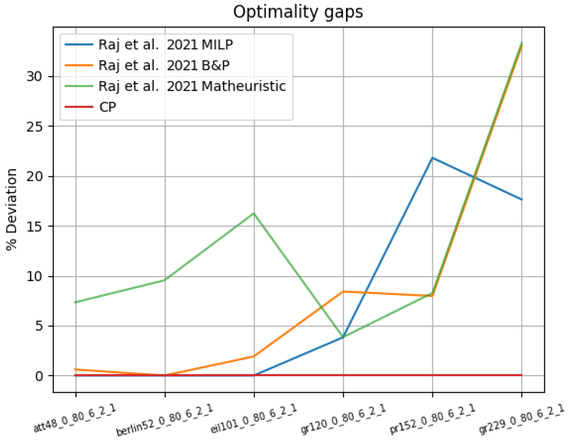
The results show that CP was able to find three new optimal solutions, with improvements of up to 15% over the previous solution values. For the hardest instances, however, significant computing time was required—more than 32 h of computation.

In Figure 4 the optimality gaps are reported for all the methods available for these instances. For each method M, the gap is calculated in terms of the percentage deviation from the optimal solution as $\frac{cost\left(M\right)-cost\left(CP\right)}{cost\left(CP\right)}·100$, where $cost\left(M\right)$ is the cost of the best solution retrieved by method M. From the chart, it is possible to see how the methods previously introduced in [13] have difficulty finding high quality solutions for the larger instances, with substantial gaps with respect to CP in some cases. From the results on these instances, the best method among those discussed in [13] appears to be the MILP-based method, although it performed poorly on one of the instances.

Table 2. Instances originated from att48 in [7]. Optimal solution costs.

Instance	Mbiadou Saleu et al. [7]—UB	Dell’Amico et al. [10]—UB	Dinh et al. [11]—UB	Lei and Chen [12]—UB	Nguyen et al. [14]—UB	Raj et al. [13]—UB	CP
							Opt Cost	Sec Found	Sec Opt
att48_0_80_1_2_1	29,954.0	29,954.0	29,954.0	29,954.0	-	-	29,954.0	0.7	1.3
att48_1_80_1_2_1	33,798.0	33,798.0	33,798.0	33,798.0	-	-	33,798.0	2.7	3.3
att48_0_0_1_2_1	42,136.0	42,136.0	42,136.0	42,136.0	-	-	42,136.0	0.3	0.3
att48_0_20_1_2_1	38,662.0	38,662.0	38,662.0	38,662.0	-	-	38,662.0	0.8	0.8
att48_0_40_1_2_1	31,592.0	31,592.0	31,592.0	31,592.0	-	-	31,592.0	0.5	0.5
att48_0_60_1_2_1	30,788.8	30,788.8	30,788.8	30,788.8	-	-	30,788.8	2.0	2.2
att48_0_100_1_2_1	27,784.0	27,784.0	27,784.0	27,784.0	-	-	27,784.0	4.1	5.2
att48_0_80_1_1_1	33,234.0	33,234.0	33,234.0	33,234.0	-	-	33,234.0	1.4	2.1
att48_0_80_1_3_1	29,142.0	29,142.0	29,142.0	29,142.0	-	-	29,142.0	2.4	5.3
att48_0_80_1_4_1	28,686.0	28,686.0	28,686.0	28,686.0	-	-	28,686.0	3.8	7.1
att48_0_80_1_5_1	28,610.0	28,610.0	28,610.0	28,610.0	-	-	28,610.0	2.9	7.6
att48_0_80_2_2_1	28,686.0	28,686.0	28,686.0	28,686.0	-	28,796.0	28,686.0	11.1	13.6
att48_0_80_3_2_1	28,610.0	28,610.0	28,610.0	28,610.0	-	-	28,610.0	2.0	18.0
att48_0_80_4_2_1	28,610.0	28,610.0	28,610.0	28,610.0	-	28,610.0	28,610.0	5.9	22.6
att48_0_80_5_2_1	28,610.0	28,610.0	28,610.0	28,610.0	-	-	28,610.0	3.5	27.3

Table 2. Instances originated from att48 in [7]. Optimal solution costs.

Instance	Mbiadou Saleu et al. [7]—UB	Dell’Amico et al. [10]—UB	Dinh et al. [11]—UB	Lei and Chen [12]—UB	Nguyen et al. [14]—UB	Raj et al. [13]—UB	CP
							Opt Cost	Sec Found	Sec Opt
att48_0_80_1_2_1	29,954.0	29,954.0	29,954.0	29,954.0	-	-	29,954.0	0.7	1.3
att48_1_80_1_2_1	33,798.0	33,798.0	33,798.0	33,798.0	-	-	33,798.0	2.7	3.3
att48_0_0_1_2_1	42,136.0	42,136.0	42,136.0	42,136.0	-	-	42,136.0	0.3	0.3
att48_0_20_1_2_1	38,662.0	38,662.0	38,662.0	38,662.0	-	-	38,662.0	0.8	0.8
att48_0_40_1_2_1	31,592.0	31,592.0	31,592.0	31,592.0	-	-	31,592.0	0.5	0.5
att48_0_60_1_2_1	30,788.8	30,788.8	30,788.8	30,788.8	-	-	30,788.8	2.0	2.2
att48_0_100_1_2_1	27,784.0	27,784.0	27,784.0	27,784.0	-	-	27,784.0	4.1	5.2
att48_0_80_1_1_1	33,234.0	33,234.0	33,234.0	33,234.0	-	-	33,234.0	1.4	2.1
att48_0_80_1_3_1	29,142.0	29,142.0	29,142.0	29,142.0	-	-	29,142.0	2.4	5.3
att48_0_80_1_4_1	28,686.0	28,686.0	28,686.0	28,686.0	-	-	28,686.0	3.8	7.1
att48_0_80_1_5_1	28,610.0	28,610.0	28,610.0	28,610.0	-	-	28,610.0	2.9	7.6
att48_0_80_2_2_1	28,686.0	28,686.0	28,686.0	28,686.0	-	28,796.0	28,686.0	11.1	13.6
att48_0_80_3_2_1	28,610.0	28,610.0	28,610.0	28,610.0	-	-	28,610.0	2.0	18.0
att48_0_80_4_2_1	28,610.0	28,610.0	28,610.0	28,610.0	-	28,610.0	28,610.0	5.9	22.6
att48_0_80_5_2_1	28,610.0	28,610.0	28,610.0	28,610.0	-	-	28,610.0	3.5	27.3

Table 3. Instances originated from berlin52 in [7]. Optimal solution costs.

Instance	Mbiadou Saleu et al. [7]—UB	Dell’Amico et al. [10]—UB	Dinh et al. [11]—UB	Lei and Chen [12]—UB	Nguyen et al. [14]—UB	Raj et al. [13]—UB	CP
							Opt Cost	Sec Found	Sec Opt
berlin52_0_80_1_2_1	6386.5	6386.5	6386.5	6386.5	-	-	6386.5	3.5	4.5
berlin52_1_80_1_2_1	7830.0	7830.0	7830.0	7830.0	-	-	7830.0	0.7	1.0
berlin52_0_0_1_2_1	9675.0	9675.0	9675.0	9675.0	-	-	9675.0	0.4	0.5
berlin52_0_20_1_2_1	9350.0	9350.0	9350.0	9350.0	-	-	9350.0	1.1	1.1
berlin52_0_40_1_2_1	8300.0	8300.0	8300.0	8300.0	-	-	8300.0	1.0	1.1
berlin52_0_60_1_2_1	7410.0	7410.0	7410.0	7410.0	-	-	7410.0	3.0	6.7
berlin52_0_100_1_2_1	6192.0	6192.0	6192.0	6192.0	-	-	6192.0	13.7	19.6
berlin52_0_80_1_1_1	7450.0	7450.0	7450.0	7450.0	-	-	7450.0	1.5	5.4
berlin52_0_80_1_3_1	5656.6	5656.6	5656.6	5656.6	-	-	5656.6	1.9	2.4
berlin52_0_80_1_4_1	5290.7	5290.7	5290.7	5290.7	-	-	5290.7	1.0	1.8
berlin52_0_80_1_5_1	5190.0	5190.0	5190.0	5190.0	-	-	5190.0	2.0	2.1
berlin52_0_80_2_2_1	5299.8	5290.7	5290.7	5290.7	-	5290.7 a	5290.7	2.8	5.3
berlin52_0_80_3_2_1	5190.0	5190.0	5190.0	5190.0	-	-	5190.0	2.2	2.2
berlin52_0_80_4_2_1	5190.0	5190.0	5190.0	5190.0	-	5190.0 a	5190.0	2.2	2.2
berlin52_0_80_5_2_1	5190.0	5190.0	5190.0	5190.0	-	-	5190.0	1.2	1.3

^a Optimality first proven in [13].

Table 3. Instances originated from berlin52 in [7]. Optimal solution costs.

Instance	Mbiadou Saleu et al. [7]—UB	Dell’Amico et al. [10]—UB	Dinh et al. [11]—UB	Lei and Chen [12]—UB	Nguyen et al. [14]—UB	Raj et al. [13]—UB	CP
							Opt Cost	Sec Found	Sec Opt
berlin52_0_80_1_2_1	6386.5	6386.5	6386.5	6386.5	-	-	6386.5	3.5	4.5
berlin52_1_80_1_2_1	7830.0	7830.0	7830.0	7830.0	-	-	7830.0	0.7	1.0
berlin52_0_0_1_2_1	9675.0	9675.0	9675.0	9675.0	-	-	9675.0	0.4	0.5
berlin52_0_20_1_2_1	9350.0	9350.0	9350.0	9350.0	-	-	9350.0	1.1	1.1
berlin52_0_40_1_2_1	8300.0	8300.0	8300.0	8300.0	-	-	8300.0	1.0	1.1
berlin52_0_60_1_2_1	7410.0	7410.0	7410.0	7410.0	-	-	7410.0	3.0	6.7
berlin52_0_100_1_2_1	6192.0	6192.0	6192.0	6192.0	-	-	6192.0	13.7	19.6
berlin52_0_80_1_1_1	7450.0	7450.0	7450.0	7450.0	-	-	7450.0	1.5	5.4
berlin52_0_80_1_3_1	5656.6	5656.6	5656.6	5656.6	-	-	5656.6	1.9	2.4
berlin52_0_80_1_4_1	5290.7	5290.7	5290.7	5290.7	-	-	5290.7	1.0	1.8
berlin52_0_80_1_5_1	5190.0	5190.0	5190.0	5190.0	-	-	5190.0	2.0	2.1
berlin52_0_80_2_2_1	5299.8	5290.7	5290.7	5290.7	-	5290.7 a	5290.7	2.8	5.3
berlin52_0_80_3_2_1	5190.0	5190.0	5190.0	5190.0	-	-	5190.0	2.2	2.2
berlin52_0_80_4_2_1	5190.0	5190.0	5190.0	5190.0	-	5190.0 a	5190.0	2.2	2.2
berlin52_0_80_5_2_1	5190.0	5190.0	5190.0	5190.0	-	-	5190.0	1.2	1.3

^a Optimality first proven in [13].

Table 4. Instances originated from eil101 in [7]. Optimal solution costs.

Instance	Mbiadou Saleu et al. [7]—UB	Dell’Amico et al. [10]—UB	Dinh et al. [11]—UB	Lei and Chen [12]—UB	Nguyen et al. [14]—UB	Raj et al. [13]—UB	CP
							Opt Cost	Sec Found	Sec Opt
eil101_0_80_1_2_1	564.0	564.0	564.0	564.0	564.0	-	564.0	34.3	39.5
eil101_1_80_1_2_1	650.0	649.0	649.0	649.0	649.0	-	649.0	71.4	80.8
eil101_0_0_1_2_1	819.0	819.0	819.0	819.0	819.0	-	819.0	5.9	6.0
eil101_0_20_1_2_1	738.0	736.0	736.0	736.0	736.0	-	736.0	15.7	20.2
eil101_0_40_1_2_1	646.0	646.0	646.0	646.0	646.0	-	646.0	21.4	38.8
eil101_0_60_1_2_1	578.0	578.0	578.0	578.0	578.0	-	578.0	31.4	35.9
eil101_0_100_1_2_1	561.4	560.0	560.0	560.0	560.0	-	560.0	54.8	92.4
eil101_0_80_1_1_1	650.0	650.0	650.0	650.0	650.0	-	650.0	70.3	92.5
eil101_0_80_1_3_1	504.0	504.0	503.9	503.2	503.2	-	503.2	22.2	44.2
eil101_0_80_1_4_1	456.0	456.0	456.0	456.0	456.0	-	456.0	16.0	36.0
eil101_0_80_1_5_1	420.8	421.0	420.8	420.8	420.8	-	420.8	29.6	35.5
eil101_0_80_2_2_1	456.0	456.0	456.0	456.0	456.0	458.8	456.0	57.7	276.0
eil101_0_80_3_2_1	395.0	395.0	395.0	395.0	395.0	-	395.0	29.9	65.9
eil101_0_80_4_2_1	346.7	346.0	346.0	346.0	346.0	354.0	346.0	25.5	36.7
eil101_0_80_5_2_1	319.7	318.0	318.0	318.0	318.0	-	318.0	11.9	33.5

Table 4. Instances originated from eil101 in [7]. Optimal solution costs.

Instance	Mbiadou Saleu et al. [7]—UB	Dell’Amico et al. [10]—UB	Dinh et al. [11]—UB	Lei and Chen [12]—UB	Nguyen et al. [14]—UB	Raj et al. [13]—UB	CP
							Opt Cost	Sec Found	Sec Opt
eil101_0_80_1_2_1	564.0	564.0	564.0	564.0	564.0	-	564.0	34.3	39.5
eil101_1_80_1_2_1	650.0	649.0	649.0	649.0	649.0	-	649.0	71.4	80.8
eil101_0_0_1_2_1	819.0	819.0	819.0	819.0	819.0	-	819.0	5.9	6.0
eil101_0_20_1_2_1	738.0	736.0	736.0	736.0	736.0	-	736.0	15.7	20.2
eil101_0_40_1_2_1	646.0	646.0	646.0	646.0	646.0	-	646.0	21.4	38.8
eil101_0_60_1_2_1	578.0	578.0	578.0	578.0	578.0	-	578.0	31.4	35.9
eil101_0_100_1_2_1	561.4	560.0	560.0	560.0	560.0	-	560.0	54.8	92.4
eil101_0_80_1_1_1	650.0	650.0	650.0	650.0	650.0	-	650.0	70.3	92.5
eil101_0_80_1_3_1	504.0	504.0	503.9	503.2	503.2	-	503.2	22.2	44.2
eil101_0_80_1_4_1	456.0	456.0	456.0	456.0	456.0	-	456.0	16.0	36.0
eil101_0_80_1_5_1	420.8	421.0	420.8	420.8	420.8	-	420.8	29.6	35.5
eil101_0_80_2_2_1	456.0	456.0	456.0	456.0	456.0	458.8	456.0	57.7	276.0
eil101_0_80_3_2_1	395.0	395.0	395.0	395.0	395.0	-	395.0	29.9	65.9
eil101_0_80_4_2_1	346.7	346.0	346.0	346.0	346.0	354.0	346.0	25.5	36.7
eil101_0_80_5_2_1	319.7	318.0	318.0	318.0	318.0	-	318.0	11.9	33.5

Table 5. Instances originated from gr120 in [7]. Optimal solution costs.

Instance	Mbiadou Saleu et al. [7]—UB	Dell’Amico et al. [10]—UB	Dinh et al. [11]—UB	Lei and Chen [12]—UB	Nguyen et al. [14]—UB	Raj et al. [13]—UB	CP
							Opt Cost	Sec Found	Sec Opt
gr120_0_80_1_2_1	1414.0	1420.8	1414.0	1414.0	1414.0	-	1414.0	168.7	206.2
gr120_1_80_1_2_1	1730.0	1726.0	1726.0	1726.0	1726.0	-	1726.0	99.0	113.6
gr120_0_0_1_2_1	2006.0	2006.0	2006.0	2006.0	2006.0	-	2006.0	7.9	8.1
gr120_0_20_1_2_1	1736.0	1736.0	1736.0	1736.0	1736.0	-	1736.0	48.1	52.0
gr120_0_40_1_2_1	1624.0	1624.0	1624.0	1624.0	1624.0	-	1624.0	142.0	152.6
gr120_0_60_1_2_1	1494.0	1494.0	1494.0	1494.0	1494.0	-	1494.0	27.5	69.8
gr120_0_100_1_2_1	1414.8	1416.0	1414.0	1414.0	1414.0	-	1414.0	138.2	775.5
gr120_0_80_1_1_1	1592.0	1592.0	1592.0	1592.0	1592.0	-	1592.0	119.7	288.1
gr120_0_80_1_3_1	1289.3	1291.0	1284.7	1284.7	1284.7	-	1284.7	75.7	97.8
gr120_0_80_1_4_1	1189.7	1192.0	1186.0	1186.0	1186.0	-	1186.0	87.4	139.7
gr120_0_80_1_5_1	1112.0	1114.0	1112.0	1112.0	1112.0	-	1112.0	91.8	403.8
gr120_0_80_2_2_1	1188.5	1197.0	1186.0	1186.0	1186.0	1202.2	1186.0	234.0	368.3
gr120_0_80_3_2_1	1044.7	1050.0	1044.0	1044.0	1044.0	-	1044.0	330.4	700.9
gr120_0_80_4_2_1	946.0	946.0	943.0	943.0	943.0	949.0	943.0	627.9	663.9
gr120_0_80_5_2_1	880.0	881.0	878.9	878.9	878.9	-	878.7	6036.6	6037.3

Table 5. Instances originated from gr120 in [7]. Optimal solution costs.

Instance	Mbiadou Saleu et al. [7]—UB	Dell’Amico et al. [10]—UB	Dinh et al. [11]—UB	Lei and Chen [12]—UB	Nguyen et al. [14]—UB	Raj et al. [13]—UB	CP
							Opt Cost	Sec Found	Sec Opt
gr120_0_80_1_2_1	1414.0	1420.8	1414.0	1414.0	1414.0	-	1414.0	168.7	206.2
gr120_1_80_1_2_1	1730.0	1726.0	1726.0	1726.0	1726.0	-	1726.0	99.0	113.6
gr120_0_0_1_2_1	2006.0	2006.0	2006.0	2006.0	2006.0	-	2006.0	7.9	8.1
gr120_0_20_1_2_1	1736.0	1736.0	1736.0	1736.0	1736.0	-	1736.0	48.1	52.0
gr120_0_40_1_2_1	1624.0	1624.0	1624.0	1624.0	1624.0	-	1624.0	142.0	152.6
gr120_0_60_1_2_1	1494.0	1494.0	1494.0	1494.0	1494.0	-	1494.0	27.5	69.8
gr120_0_100_1_2_1	1414.8	1416.0	1414.0	1414.0	1414.0	-	1414.0	138.2	775.5
gr120_0_80_1_1_1	1592.0	1592.0	1592.0	1592.0	1592.0	-	1592.0	119.7	288.1
gr120_0_80_1_3_1	1289.3	1291.0	1284.7	1284.7	1284.7	-	1284.7	75.7	97.8
gr120_0_80_1_4_1	1189.7	1192.0	1186.0	1186.0	1186.0	-	1186.0	87.4	139.7
gr120_0_80_1_5_1	1112.0	1114.0	1112.0	1112.0	1112.0	-	1112.0	91.8	403.8
gr120_0_80_2_2_1	1188.5	1197.0	1186.0	1186.0	1186.0	1202.2	1186.0	234.0	368.3
gr120_0_80_3_2_1	1044.7	1050.0	1044.0	1044.0	1044.0	-	1044.0	330.4	700.9
gr120_0_80_4_2_1	946.0	946.0	943.0	943.0	943.0	949.0	943.0	627.9	663.9
gr120_0_80_5_2_1	880.0	881.0	878.9	878.9	878.9	-	878.7	6036.6	6037.3

Table 6. Instances originated from pr152 in [7]. Optimal solution costs.

Instance	Mbiadou Saleu et al. [7]—UB	Dell’Amico et al. [10]—UB	Dinh et al. [11]—UB	Lei and Chen [12]—UB	Nguyen et al. [14]—UB	Raj et al. [13]—UB	CP
							Opt Cost	Sec Found	Sec Opt
pr152_0_80_1_2_1	76,008.0	76,008.0	76,008.0	76,008.0	76,008.0	-	76,008.0	316.2	324.4
pr152_1_80_1_2_1	76,556.0	76,556.0	76,556.0	76,556.0	76,556.0	-	76,556.0	259.8	1045.9
pr152_0_0_1_2_1	86,596.0	86,596.0	86,596.0	86,596.0	86,596.0	-	86,596.0	29.8	42.1
pr152_0_20_1_2_1	82,504.0	82,504.0	82,504.0	82,504.0	82,504.0	-	82,504.0	622.3	1120.8
pr152_0_40_1_2_1	77,372.0	77,316.0	77,236.0	77,236.0	77,236.0	-	77,236.0	23.5	39.8
pr152_0_60_1_2_1	76,786.0	76,786.0	76,786.0	76,786.0	76,758.0	-	76,758.0	47.0	74.1
pr152_0_100_1_2_1	74,468.0	74,302.0	74,302.0	74,302.0	74,302.0	-	74,302.0	708.5	775.0
pr152_0_80_1_1_1	80,164.0	79,952.0	79,952.0	79,952.0	79,952.0	-	79,952.0	94.3	106.0
pr152_0_80_1_3_1	72,936.0	72,936.0	72,936.0	72,936.0	72,936.0	-	72,936.0	243.8	398.1
pr152_0_80_1_4_1	70,412.0	70,328.0	70,148.0	70,148.0	70,148.0	-	70,148.0	431.2	553.7
pr152_0_80_1_5_1	67,798.0	67,798.0	67,798.0	67,798.0	67,858.0	-	67,798.0	1472.0	2260.9
pr152_0_80_2_2_1	70,244.0	70,405.5	70,148.0	70,148.0	70,148.0	79,686.0	70,148.0	195.4	483.6
pr152_0_80_3_2_1	65,062.1	64,720.3	64,626.0	64,550.9	64,550.0	-	64,550.0	393.4	575.6
pr152_0_80_4_2_1	60,027.4	59,772.0	59,772.0	59,772.0	59,756.0	63,990.0	59,756.0	325.4	366.8
pr152_0_80_5_2_1	56,336.1	56,262.0	56,262.0	56,180.0	56,178.0	-	56,178.0	742.9	941.0

Table 6. Instances originated from pr152 in [7]. Optimal solution costs.

Instance	Mbiadou Saleu et al. [7]—UB	Dell’Amico et al. [10]—UB	Dinh et al. [11]—UB	Lei and Chen [12]—UB	Nguyen et al. [14]—UB	Raj et al. [13]—UB	CP
							Opt Cost	Sec Found	Sec Opt
pr152_0_80_1_2_1	76,008.0	76,008.0	76,008.0	76,008.0	76,008.0	-	76,008.0	316.2	324.4
pr152_1_80_1_2_1	76,556.0	76,556.0	76,556.0	76,556.0	76,556.0	-	76,556.0	259.8	1045.9
pr152_0_0_1_2_1	86,596.0	86,596.0	86,596.0	86,596.0	86,596.0	-	86,596.0	29.8	42.1
pr152_0_20_1_2_1	82,504.0	82,504.0	82,504.0	82,504.0	82,504.0	-	82,504.0	622.3	1120.8
pr152_0_40_1_2_1	77,372.0	77,316.0	77,236.0	77,236.0	77,236.0	-	77,236.0	23.5	39.8
pr152_0_60_1_2_1	76,786.0	76,786.0	76,786.0	76,786.0	76,758.0	-	76,758.0	47.0	74.1
pr152_0_100_1_2_1	74,468.0	74,302.0	74,302.0	74,302.0	74,302.0	-	74,302.0	708.5	775.0
pr152_0_80_1_1_1	80,164.0	79,952.0	79,952.0	79,952.0	79,952.0	-	79,952.0	94.3	106.0
pr152_0_80_1_3_1	72,936.0	72,936.0	72,936.0	72,936.0	72,936.0	-	72,936.0	243.8	398.1
pr152_0_80_1_4_1	70,412.0	70,328.0	70,148.0	70,148.0	70,148.0	-	70,148.0	431.2	553.7
pr152_0_80_1_5_1	67,798.0	67,798.0	67,798.0	67,798.0	67,858.0	-	67,798.0	1472.0	2260.9
pr152_0_80_2_2_1	70,244.0	70,405.5	70,148.0	70,148.0	70,148.0	79,686.0	70,148.0	195.4	483.6
pr152_0_80_3_2_1	65,062.1	64,720.3	64,626.0	64,550.9	64,550.0	-	64,550.0	393.4	575.6
pr152_0_80_4_2_1	60,027.4	59,772.0	59,772.0	59,772.0	59,756.0	63,990.0	59,756.0	325.4	366.8
pr152_0_80_5_2_1	56,336.1	56,262.0	56,262.0	56,180.0	56,178.0	-	56,178.0	742.9	941.0

Table 7. Instances originated from gr229 in [7]. Optimal solution costs.

Instance	Mbiadou Saleu et al. [7]—UB	Dell’Amico et al. [10]—UB	Dinh et al. [11]—UB	Lei and Chen [12]—UB	Nguyen et al. [14]—UB	Raj et al. [13]—UB	CP
							Opt Cost	Sec Found	Sec Opt
gr229_0_80_1_2_1	1794.8	1785.9	1781.2	1783.1	1780.9	-	1780.9	1697.6	1817.6
gr229_1_80_1_2_1	1913.7	1911.6	1911.6	1911.6	1911.6	-	1911.6	2084.8	2355.3
gr229_0_0_1_2_1	2020.2	2017.2	2017.2	2017.2	2017.2	-	2017.2	125.6	127.7
gr229_0_20_1_2_1	1862.8	1860.1	1860.1	1860.1	1860.1	-	1860.1	279.4	316.1
gr229_0_40_1_2_1	1828.0	1827.0	1824.8	1825.9	1824.8	-	1824.8	1517.3	1595.4
gr229_0_60_1_2_1	1807.5	1797.4	1796.9	1796.6	1796.6	-	1796.6	691.8	794.1
gr229_0_100_1_2_1	1498.1	1496.3	1697.0	1496.3	1496.3	-	1496.3	316.4	358.9
gr229_0_80_1_1_1	1865.0	1863.1	1862.0	1862.0	1862.0	-	1862.0	558.5	723.8
gr229_0_80_1_3_1	1735.2	1725.5	1717.9	1719.9	1716.7	-	1716.7	806.8	1371.6
gr229_0_80_1_4_1	1679.3	1675.8	1668.1	1669.9	1664.8	-	1664.8	2748.8	3940.5
gr229_0_80_1_5_1	1642.0	1629.4	1623.1	1622.9	1620.2	-	1620.2	1895.6	2434.2
gr229_0_80_2_2_1	1686.8	1673.7	1668.3	1666.9	1664.8	1851.5	1664.8	2139.1	3644.9
gr229_0_80_3_2_1	1603.9	1592.5	1582.9	1582.4	1580.9	-	1580.9	4103.6	6480.7
gr229_0_80_4_2_1	1518.6	1526.9	1516.7	1515.1	1511.7	1899.9	1511.7	6109.2	7528.1
gr229_0_80_5_2_1	1483.7	1467.8	1465.0	1460.7	1458.7	-	1458.7	15,361.5	17,367.1

Table 7. Instances originated from gr229 in [7]. Optimal solution costs.

Instance	Mbiadou Saleu et al. [7]—UB	Dell’Amico et al. [10]—UB	Dinh et al. [11]—UB	Lei and Chen [12]—UB	Nguyen et al. [14]—UB	Raj et al. [13]—UB	CP
							Opt Cost	Sec Found	Sec Opt
gr229_0_80_1_2_1	1794.8	1785.9	1781.2	1783.1	1780.9	-	1780.9	1697.6	1817.6
gr229_1_80_1_2_1	1913.7	1911.6	1911.6	1911.6	1911.6	-	1911.6	2084.8	2355.3
gr229_0_0_1_2_1	2020.2	2017.2	2017.2	2017.2	2017.2	-	2017.2	125.6	127.7
gr229_0_20_1_2_1	1862.8	1860.1	1860.1	1860.1	1860.1	-	1860.1	279.4	316.1
gr229_0_40_1_2_1	1828.0	1827.0	1824.8	1825.9	1824.8	-	1824.8	1517.3	1595.4
gr229_0_60_1_2_1	1807.5	1797.4	1796.9	1796.6	1796.6	-	1796.6	691.8	794.1
gr229_0_100_1_2_1	1498.1	1496.3	1697.0	1496.3	1496.3	-	1496.3	316.4	358.9
gr229_0_80_1_1_1	1865.0	1863.1	1862.0	1862.0	1862.0	-	1862.0	558.5	723.8
gr229_0_80_1_3_1	1735.2	1725.5	1717.9	1719.9	1716.7	-	1716.7	806.8	1371.6
gr229_0_80_1_4_1	1679.3	1675.8	1668.1	1669.9	1664.8	-	1664.8	2748.8	3940.5
gr229_0_80_1_5_1	1642.0	1629.4	1623.1	1622.9	1620.2	-	1620.2	1895.6	2434.2
gr229_0_80_2_2_1	1686.8	1673.7	1668.3	1666.9	1664.8	1851.5	1664.8	2139.1	3644.9
gr229_0_80_3_2_1	1603.9	1592.5	1582.9	1582.4	1580.9	-	1580.9	4103.6	6480.7
gr229_0_80_4_2_1	1518.6	1526.9	1516.7	1515.1	1511.7	1899.9	1511.7	6109.2	7528.1
gr229_0_80_5_2_1	1483.7	1467.8	1465.0	1460.7	1458.7	-	1458.7	15,361.5	17,367.1

Table 8. Instances originated from TSPLIB in [13]. Optimal solution costs.

Instances	Raj et al. [13] MILP UB	Raj et al. [13] B&P UB	Raj et al. [13] Matheuristic UB	CP
				Opt Cost	Sec Found	Sec Opt
att48_0_80_6_2_1	28,610.0	28,784.0	30,708.0	28,610.0	9.8	43.0
berlin52_0_80_6_2_1	5190.0 a	5190.0	5685.0	5190.0	4.8	4.9
eil101_0_80_6_2_1	314.0	320.0	365.0	314.0	43.6	78.2
gr120_0_80_6_2_1	851.4	889.0	851.5	820.0	666.9	2232.0
pr152_0_80_6_2_1	65,140.0	57,794.0	57,794.0	53,478.0	1401.2	1446.9
gr229_0_80_6_2_1	1664.6	1883.8	1883.8	1415.1	3214.2	115,622.3

^a Optimality first proven in [13].

Table 8. Instances originated from TSPLIB in [13]. Optimal solution costs.

Instances	Raj et al. [13] MILP UB	Raj et al. [13] B&P UB	Raj et al. [13] Matheuristic UB	CP
				Opt Cost	Sec Found	Sec Opt
att48_0_80_6_2_1	28,610.0	28,784.0	30,708.0	28,610.0	9.8	43.0
berlin52_0_80_6_2_1	5190.0 a	5190.0	5685.0	5190.0	4.8	4.9
eil101_0_80_6_2_1	314.0	320.0	365.0	314.0	43.6	78.2
gr120_0_80_6_2_1	851.4	889.0	851.5	820.0	666.9	2232.0
pr152_0_80_6_2_1	65,140.0	57,794.0	57,794.0	53,478.0	1401.2	1446.9
gr229_0_80_6_2_1	1664.6	1883.8	1883.8	1415.1	3214.2	115,622.3

^a Optimality first proven in [13].

5. Conclusions

The aim of the investigation was to show the potential of constraint programming solvers on optimization problems that—like the parallel drone scheduling traveling salesman problem—extend the concepts of a traditional traveling salesman problem. The new constraint programming model we propose leads—by exploiting multi-threading computation—to a very effective exact algorithm for the problem considered. The method was able to find the optimal solution for all the instances normally considered in the literature, and this was the first optimality proof for most of the instances. During the process, four of the previously best-known solution costs were also improved.

Finally, we believe that straightforward adaptations of the model we propose could lead to state-of-the-art results for many of the several extensions proposed to the basic problem considered here, although this is beyond the scope of the present paper. From a more general perspective, we also believe that constraint programming has potential for use in effectively attacking many other optimization problems arising in different fields.