Union Models for Model Families: Efficient Reasoning over Space and Time

Abstract

A model family is a set of related models in a given language, with commonalities and variabilities that result from evolution of models over time and/or variation over intended usage (the spatial dimension). As the family size increases, it becomes cumbersome to analyze models individually. One solution is to represent a family using one global model that supports analysis. In this paper, we propose the concept of union model as a complete and concise representation of all members of a model family. We use graph theory to formalize a model family as a set of attributed typed graphs in which all models are typed over the same metamodel. The union model is formalized as the union of all graph elements in the family. These graph elements are annotated with their corresponding model versions and configurations. This formalization is independent from the modeling language used. We also demonstrate how union models can be used to perform reasoning tasks on model families, e.g., trend analysis and property checking. Empirical results suggest potential time-saving benefits when using union models for analysis and reasoning over a set of models all at once as opposed to separately analyzing single models one at a time.

1. Introduction

Model-based Software Engineering (MBSE) is a software engineering paradigm that endorses the use of models as first-class artifacts [1]. A model can be defined with a domain-specific modeling language (DSML) [2], which provides modeling primitives to capture the semantics of a specific application domain (such as web-based languages) or can be defined using a general-purpose modeling language (such as the UML). The main goal of MBSE is to enhance the development, maintenance, and evolution of complex software systems by raising the level of abstraction from source code to models. In particular, the use of DSMLs allows developers to focus on their essential tasks while the recurring engineering tasks are lifted to higher abstraction levels and automatically generated by transformations specified by domain experts [3]. The use of the MBSE paradigm is beneficial because it allows engineers to focus on the product to be developed and on generic and reusable assets that express problems and solutions. Other measured or claimed benefits of MBSE include better communication, effectiveness, and quality compared to pure code-oriented approaches [4,5].

In MBSE, models expressed using any modeling language often undergo continuous evolution during their lifecycles. For example, such evolution can occur when new requirements are added or existing requirements are changed as engineers gain better understanding of the domain to be modeled. Models can evolve over time, resulting in a family of related models, which we refer to as a model family, with differences and similarities between family members. Another common source of model families is found in (software) product lines, where different configurations of a product can exist simultaneously (i.e., in the same space dimension) for different customers without necessarily being caused by evolution over time. Model families can result from having several alternatives due to design-time uncertainty or uncertainty at other stages of the development process. In such cases, all models need to exist together (as a model family) to tolerate a certain level of uncertainty until decisions absolutely need to be made [6]. Finally, a model family can appear as a result of both evolution over time and variation over space, such in the case of a set of software/product configurations that evolve over time [7].

The phenomenon of model families can be observed in several domains, including the regulatory domain, where regulations evolve over time and have variations (e.g., for different regulated parties or different versions of regulations) that need to be modeled using slightly different individual models, resulting in a family of related regulatory models [8,9]. In regulatory domains it is usually desirable to analyze models, for instance, for compliance assessment by regulators. However, the existence of several versions/variations of models makes it cumbersome and inefficient to analyze and reason about these models one at a time. This challenge was observed in practice through our previous experience in modeling and analyzing safety regulations at Transport Canada; the number of models in a model family can be very large due to multiple versions and variations that nonetheless share many elements in common. Exploiting this redundancy during analysis has the potential to reduce the effort and time required for analysis.

This paper is based on the first author’s PhD thesis [10], and proposes union models as first-class generic artifacts to: (1) support the representation of model families (for time and space dimensions) using one generic model; (2) achieve performance gains during analysis of model families all at once, compared to analysis of individual models, one model at a time; and (3) support types of analyses that are more easily feasible with union models compared with individual models.

The use of union models is challenging and non-trivial. At the model level, the challenges stem mainly from the following requirements:

Req. 1

Models in a family shall be captured (in both dimensions of variability) in a complete and exact way such that all and only individual members of a family are included in one union model.

Req. 2

The resulting union model shall be as compact as possible, in the sense that it should not contain redundant elements, especially when there are many elements in common between models.

Req. 3

The union model shall be self-explanatory, i.e., it should be supported with a mechanism that distinguishes which elements belong to which models.

There are other challenges at the metamodel level associated with the use of union models. In particular, a union model may not be a valid instance of the language’s metamodel, and the latter might need to have its constraints relaxed accordingly. The metamodel-level challenges have been already discussed in our previous work [11], and are outside the scope of this paper.

This paper extends previous work in [12] with a complete formalization of union models, including annotations, and enhanced experiments with a deeper analysis, and empirically demonstrates the usefulness of union models for analyzing a family of models all at once compared to individual models one model at a time. The main contributions of this paper are:

1.

A language-independent graph-based formalization of model families and union models;

2.

A generic language-independent algorithm to produce a union model from a set of models (in a compact and exact manner) in a given language (satisfying Req. 1 and Req. 2);

3.

A Spatio-Temporal Annotation Language (STAL) to support the representation of variability in model families in the space and time dimensions and to facilitate reasoning about union models (satisfying Req. 3); and

4.

Improved efficiency of analysis and reasoning over a set of models all at once using union models, compared to reasoning on single models one model at a time.

As our approach starts with existing models as input, how such models are constructed in general is beyond the scope of this paper.

From a methodological perspective, this paper first presents the motivation behind this work in Section 2. Then, the theoretical and algorithmic foundations of our work are presented in the next three chapters, specifically, a graph-based formalization of model families (Section 3), a complementary Spatio-Temporal Annotation Language (Section 4), and the propositional encoding of models (Section 5). To determine how efficient and beneficial the reasoning and analysis with union models are, reasoning tasks and the experimental setup are first presented in Section 6, whereas empirical results and threats to validity are reported in Section 7. A discussion of closely related works is covered in Section 8. Finally, Section 9 concludes the paper.

2. Motivation

This work was inspired by issues faced previously with regulation modeling in collaboration with Transport Canada, where there are regulations that evolve over time and that apply to different types of organizations (i.e., spaces). We explain the challenges associated with regulatory model families and motivate our proposed solution using a running example from this domain, namely, airports regulated by Transport Canada, where we use the Goal-oriented Requirement Language (GRL) as a modeling language. GRL is a part of the User Requirements Notation (URN) standard [13].

Without loss of generality, the subsequent discussion about GRL model families in regulatory domains and their challenges is applicable to other model families from modeling languages other than the GRL. Therefore, we posit that our approach is feasible for any metamodel-based modeling languages and their model families.

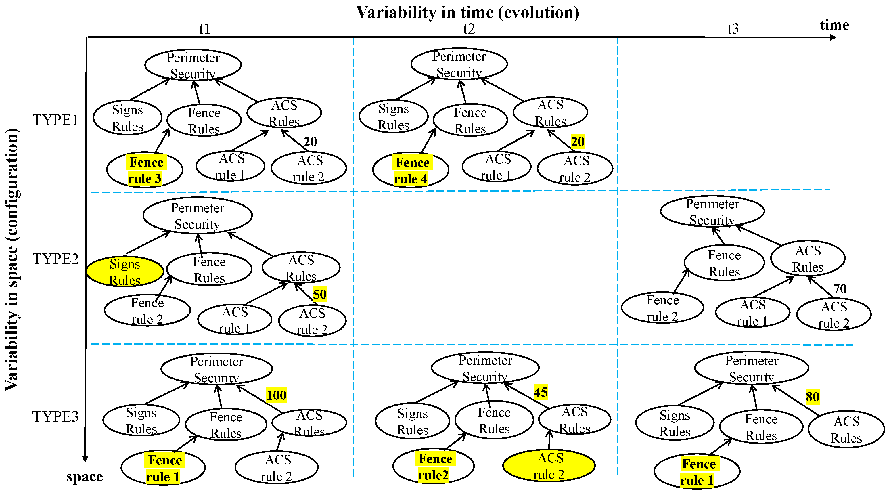
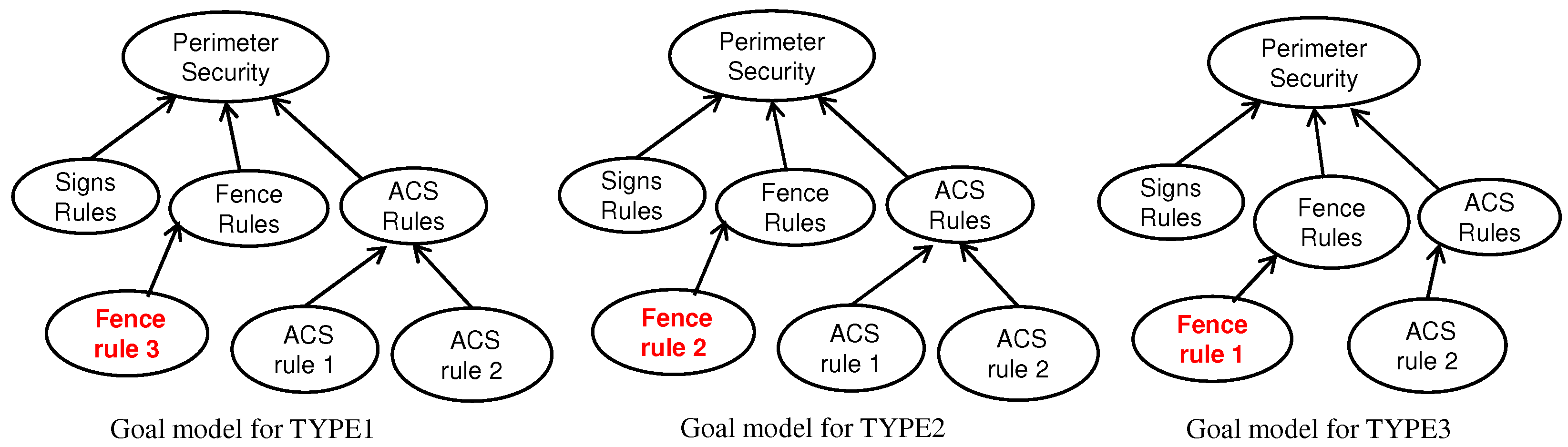
At Transport Canada there are many regulations that need to be modeled by regulators, for example, to enable compliance and performance assessments. These regulations evolve over time, and apply to multiple types of organizations (such as aerodromes and airlines) of different sizes [8,9]. For example, as Figure 1 shows, certain rules/regulations apply differently depending on the targeted aerodrome type (configurations modeled abstractly here as TYPE1, TYPE2, and TYPE3), while other regulations are only applicable to specific aerodrome types. In Figure 1, regulations related to Fence rule 3 are only applicable to aerodrome TYPE1, Access Control System (ACS) rule 2 is applicable to all aerodrome types, and ACS rule 1 is applicable to TYPE1 and TYPE2 aerodromes but not to TYPE3 ones.

The different aerodrome types (i.e., TYPE1, TYPE2, and TYPE3) can be considered as different configurations (or spaces) that are available at the same time for different aerodromes. This means that the three goal model variations depicted in Figure 1 represent a goal model family along the space dimension, where each space has different regulations. Goal models in this family can evolve over time, e.g., when the regulatory context evolves, resulting in several versions of the same model. Evolution of goal models can involve the addition/deletion of goals and/or links or modifications to attributes of goals and/or links, as illustrated in each row of Figure 2. In this figure, the time-related changes across each of the initial configuration models (from Figure 1) are highlighted in Yellow.

Analyzing the different versions/variations of models in Figure 2 individually using one goal model per type of aerodrome and at each time instance is impractical for the following reasons:

1.

If a modeler plans to conduct goal satisfaction analysis (using some GRL forward propagation algorithm [13]) on each individual model by running a strategy that initially assigns ACS rule 2 to study the impact of its satisfaction on the satisfaction of other goals, she would end up running the same evaluation algorithm six times for this example, even though there are several common elements among the seven models. Intuitively, if there are M individual models in a model family and each model has E elements, then the complexity of running a satisfaction propagation algorithm on all models would be on the order of $\mathcal{O}(M\times E)$. Such complexity becomes more significant if there are hundreds of models with hundreds of elements in each model, which is not an atypical situation.

2.

Each individual model (e.g., goal model for TYPE1 at time t1) does not represent the whole set of regulations per se. Hence, a regulator who wishes to reason about all regulations (e.g., to study the evolution trend of regulations over time) would have to check all models one model at a time and reason about each one separately. This process becomes inefficient and time consuming as the number of models increases.

3.

Models in a model family are subject to frequent evolution over time that are asynchronous by nature. Such asynchronous evolution sometimes requires that older versions of models (which represent legacy models) need to be maintained, as they may remain in use even after being superseded by newer versions. This is an issue over the time dimension, and can be witnessed in the space dimension as well (i.e., along configurations). In this scenario, legacy models and new models need to co-exist together in one model in order to be analyzed together.

Similar challenges exist in the software engineering field, particularly in the Software Product Line (SPL) domain, where products vary over the space dimension and may evolve over time as well. By nature, an SPL encodes a set of related product variants; thus, dealing with the evolution of multiple products over time means that developers should consider an additional dimension of variability by reasoning about sets of products. This combination of variation and evolution is not well supported by existing SPL engineering techniques, and only a few recent approaches in the literature have tried to address this issue. For example, Seidl et al. [14] and Lity et al. [15] considered variation of SPLs in space and time and proposed a so-called 175% modeling formalism to allow for the development and documentation of evolving product lines. In their paper, they urged the community to extend annotative variability modeling to tackle evolution and variation by the same means. Famelis et al. [16] proposed an approach for combining SPLs with partial models to represent design-time uncertainty. The resulting artifact, called Software Product Lines with Design Choices (SPLDCs), integrates variability and design-time uncertainty in a common formalism to help developers differentiate between the kinds of decisions that are relevant during the design and configuration stages of the SPL lifecycle.

The above-mentioned three challenges (especially the first one) and the gaps identified in the literature motivate the need to find a way to represent model families other than using separate individual models. This paper proposes union models ($M_U$) as a generic modeling artifact to capture all model elements in all members of a model family $\mathit{MF}$, aggregated in a compact and exact way such that analysis of a group of models is faster than for individual models and where members of a family can be extracted and analyzed. Generally speaking, a union model $M_U$ of any potential model family would be the union of all elements e in all individual models $M_i$ of the family $\mathit{MF}$; that is,

$$M_U=(\bigcup _{i=1}^{\left|\mathit{MF}\right|}\bigcup _{j=1}^{|M_i|}{e}_{i,j})$$

(1)

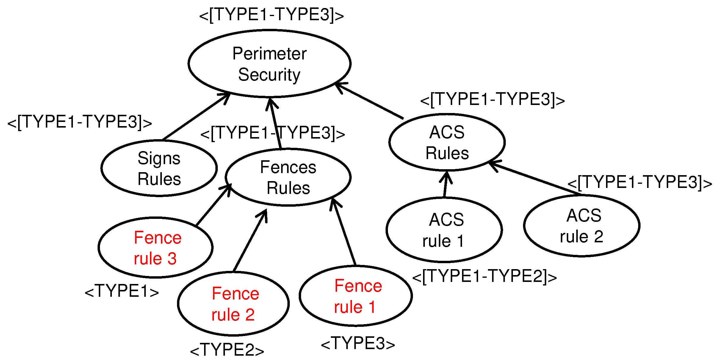
In addition, the elements of the resulting union model need to be annotated in a way that enables the identification of variants. For illustration purposes, an $M_U$ that captures the model family shown in Figure 1 is represented in Figure 3, with all elements (i.e., goal and links) of the union model included and annotated with space information (TYPES in this example) to distinguish which element belongs to which model variant.

Note that each member of the model family is embedded in the union model, i.e., for each $M_i\in MF$ there exists an embedding $i:M_i\to M_U$ defined by $i\left(e\right)=e$. Moreover, we can retract any model $M_i$ in the family from the union model by the partial mapping $r_i:M_U\to M_i$, where $r_i\left(e\right)=e$ if e is annotated with $M_i$ and is undefined otherwise. Hence, the union model is complete in the sense that it includes all information available in any member of the modeling family, and is complete in the sense that we can reconstruct each member of modeling family from it.

3. Formalization of Model Families

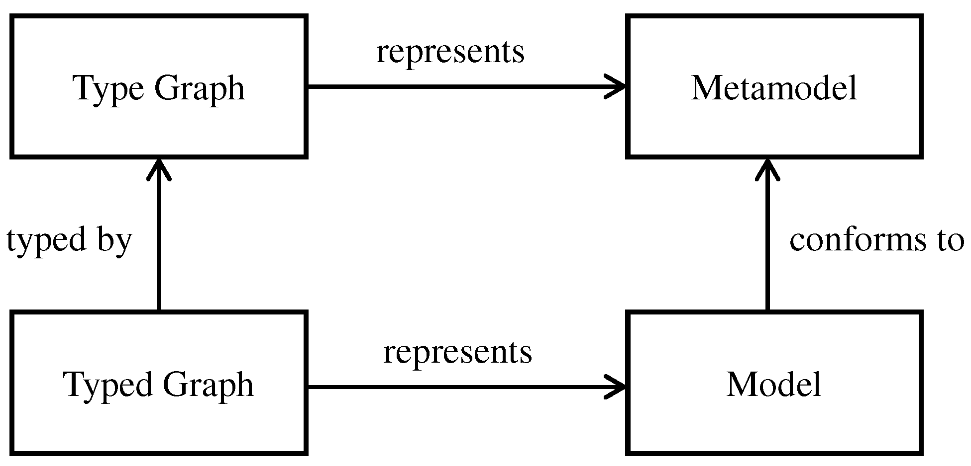
This section illustrates the use of graphs and type(d) graphs to formalize basic (meta)modeling concepts. Figure 4 illustrates the basic relationships between models and metamodels and their graphical representation. The definitions of graphs and type/typed graphs are then used as a basis for further formal definitions of model families and their union models. To model more detailed aspects of model families, we extend the definitions of basic type(d) graphs with attributes (i.e., attributed type graphs, or E-graphs [17]). The definitions that follow are based on [18,19,20].

Definition 1.

Graph: A graph is a tuple G = (N_G, E_G, src_G, tgt_G), where N_G is a set of graph nodes (or vertices), E_G is a set of graph edges, and functions src_G, tgt_G: E_G → N_G associate to each edge a source and a target node, respectively, such that e: x → y denotes an edge e with src_G(e) = x and tgt_G(e) = y.

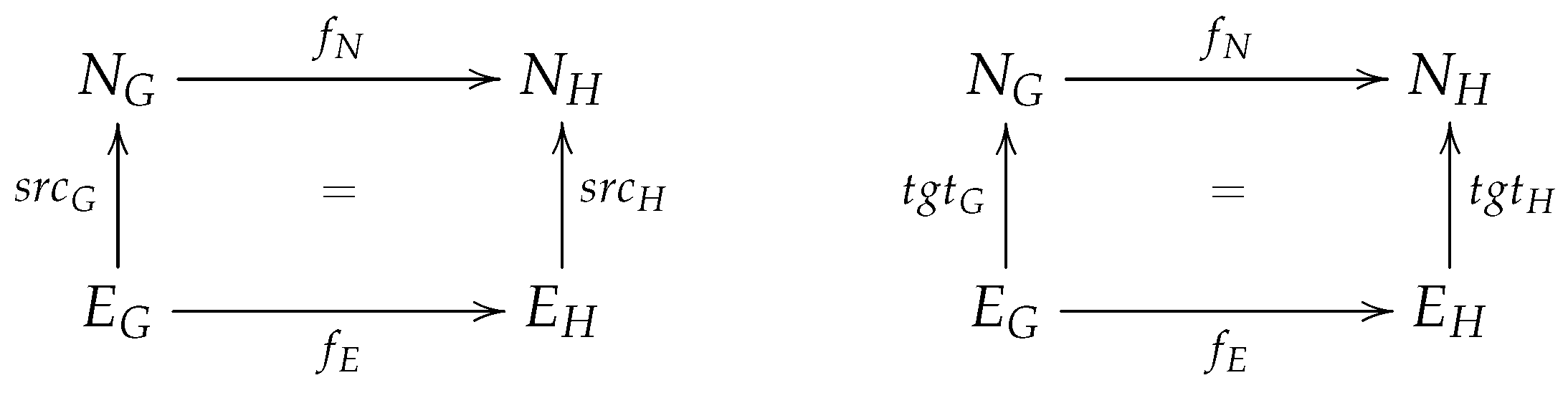
Definition 2.

Graph morphism: Let G and H be two graphs. A graph morphism f: G → H consists of a pair of functions (f_N, f_E) with f_N: N_G → N_H and f_E: E_G → E_H that preserves sources and targets of edges when composed (∘), i.e., f_N∘ src_G = src_H∘ f_E and f_N∘ tgt_G = tgt_H∘ f_E. In other words, for each edge e_G ∈ E_G there is a corresponding edge e_H = f_E(e_G) ∈ E_H such that src_G(e_G) is mapped to src_H(e_H) and tgt_G(e_G) is mapped to tgt_H(e_H). This is illustrated in Figure 5.

3.1. Type Graphs and Typed Graphs

In graph theory (such as in strongly-typed programming languages, where each constant or variable is assigned a data type), it is often useful to determine the well-formedness of a graph by checking whether it conforms to a so-called type graph. A type graph is a distinguished graph containing all the relevant types and their interrelations [21]. This is analogous to the relationship between models and metamodels in the model-driven engineering world, where each model (e.g., a UML design model) needs to conform to a metamodel (e.g., of the UML language). The correspondence between both ideas is depicted in Figure 4.

Definition 3.

Type graph (metamodel): A type graph TG is a distinguished graph, where TG = (N_TG, E_TG, src_TG, tgt_TG), and N_TG and E_TG are types of nodes and edges, respectively.

Definition 4.

Typed graph (model): A typed graph is a triple G_typed = (G, type, TG) such that G is a graph (Definition 1) and type: G → TG is a graph morphism (Definition 2) called the typing morphism. The typed graph G_typed is called an instance (graph) of (the graph) TG, and we denote the set of all instance graphs of TG as Inst[TG].

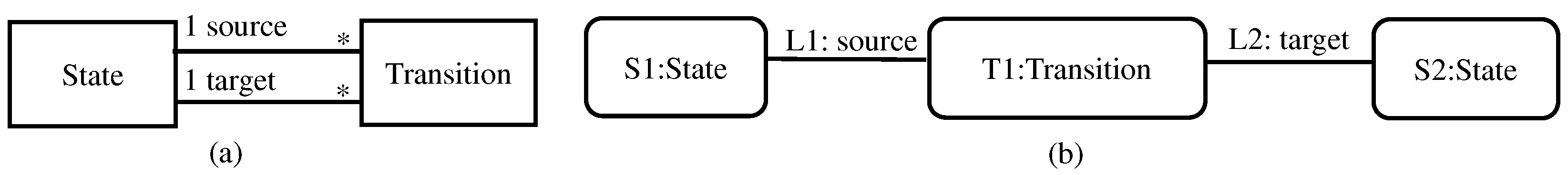
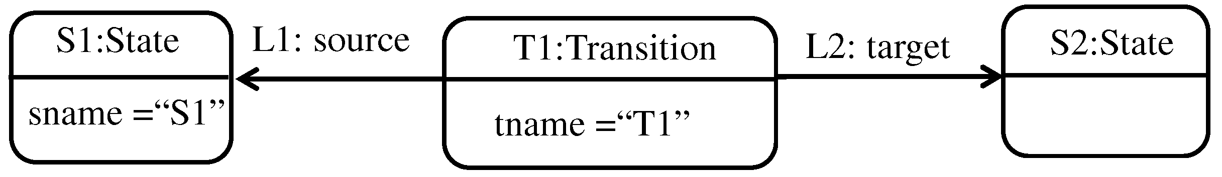
Figure 6b shows an example of a typed graph typed over the type graph to its left (Figure 6a). The type graph in Figure 6a represents the types of nodes and edges. There are two types of nodes here, namely, State and Transition, and two types of association edges, namely, source and target. Node names and types in the typed graph are depicted inside the nodes as name: type. For instance, in the node labeled with S1: State, S1 is the name of a node and State is the type of that node. For the edges, names and types of edges are represented in the same way.

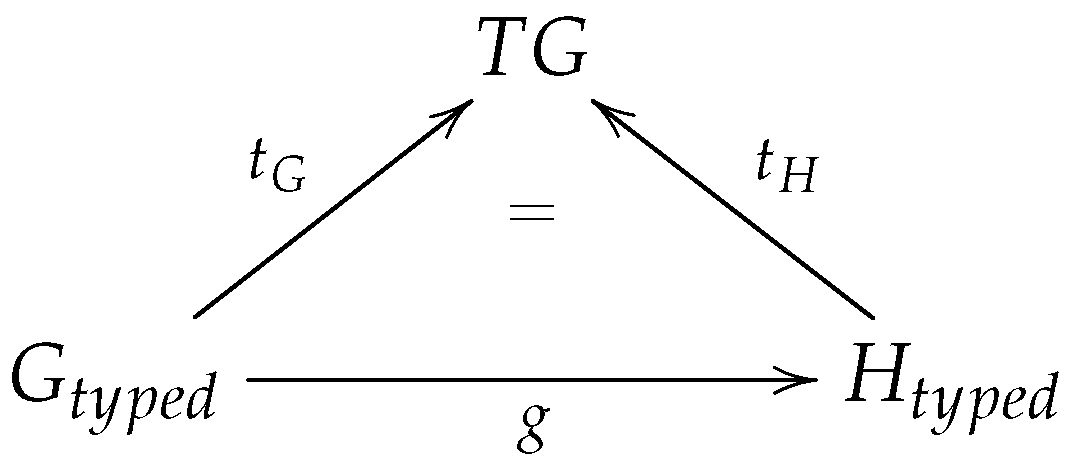
Definition 5.

Typed graph morphism: Given a type graph TG, and two typed graphs G_typed and H_typed (typed over TG), a typed graph morphism g: (G_typed, t_G: G_typed → TG) → (H_typed, t_H: H_typed$\to$ TG) is a graph morphism g: G_typed → H_typed that also preserves typing, i.e., g ∘ t_H = t_G, as illustrated in Figure 7.

3.2. Attributed Type(d) Graphs as E-Graphs

Given a typed graph (i.e., a model), it is useful in practice to attach additional information to nodes and edges by attributing them, such that each node and/or edge can contain zero or more attributes. In this case, we refer to typed attributed graphs, where attributes are typically a name:value pair that allows to attach a specific value to each attribute name. In addition, given a typed attributed graph that is typed over some TG (i.e., a metamodel), that TG needs to constrain the names and types of attributes that are allowed for certain types of nodes and edges. 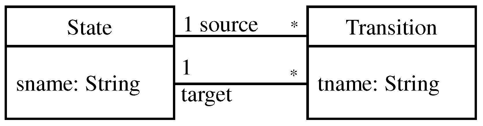In this context, we refer to an Attributed Type Graph (ATG), as shown in Figure 8, which extends the type graph illustrated in Figure 6a with node attributes.

As an example of a typed attributed graph, reconsider the typed graph in Figure 6b extended with attributes as in Figure 9, where nodes have attributes with names tname, sname.

In this paper, we adopt the definition of Ehrig et al. [22] for E-graphs to represent ATGs (note that from now on in this paper, the concept of ATG implicitly means an attributed type graph that is represented as an E-graph), which allows attribution for both nodes and edges, where attributes of nodes (resp. edges) are represented as special edges between graph nodes (resp. graph edges) and data nodes that represent the data types of these attributes. 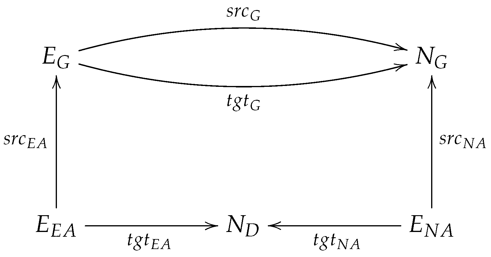Figure 10 visualizes the concept of E-graphs.

Definition 6.

E-graph: An E-graph is a tuple EG = (N_G, N_D, E_G, E_NA, E_EA, (src_j, tgt_j) j ∈ {G, NA, EA}) where:

• N_G and N_D are graph nodes and data nodes, respectively;
• E_G, E_NA, and E_EA are graph edges, node attribute edges, and edge attribute edges, respectively;
• src_j and tgt_j, where j $\in \{$G, NA, EA} are source and target functions that assign to each of the three categories of edges (i.e., E_G, E_NA, and E_EA) a source and a target, as follows:

  –

  src_G: E_G → N_G, tgt_G: E_G → N_G for graph edges;

  –

  src_NA: E_NA → N_G, tgt_NA: E_NA → N_D for node attribute edges;

  –

  src_EA: E_EA → E_G, tgt_EA: E_EA → N_D for edge attribute edges.

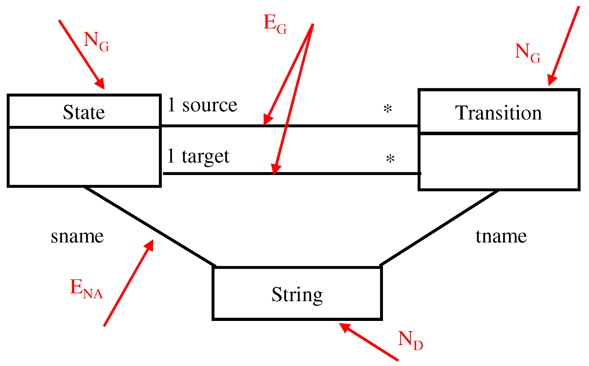
Example: 

The ATG in Figure 8 is represented as the E-graph illustrated in Figure 11. The figure shows the different categories of nodes and edges defined in Definition 6, namely:

• Graph nodes (N_G): State, Transition
• Data nodes (N_D): String
• Graph edges (E_G): source, target
• Node attribute edges (E_NA): sname, tname

Figure 11. An E-Graph, EG, with node attributes represented as edges. The star (*) indicates that zero or more instances of the class “Transition” are associated with one instance of the class “State”.

Figure 11. An E-Graph, EG, with node attributes represented as edges. The star (*) indicates that zero or more instances of the class “Transition” are associated with one instance of the class “State”.

In addition, attributes of nodes are represented as special edges between graph nodes and data nodes that represent the type that attributes. For example, the attribute tname is represented as an edge between graph node Transition and the data node String.

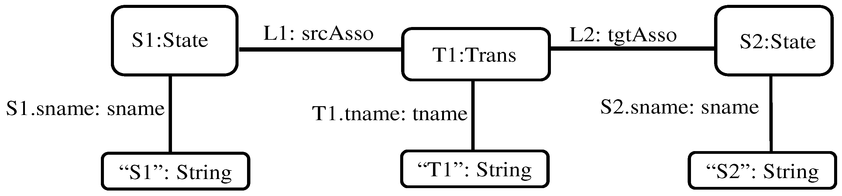
An instance typed graph ITG (i.e., model) of the attributed E-graph EG in Figure 11 is illustrated in Figure 12, where this figure is a representation of the typed attributed graph found in Figure 9. We use the notation Inst[EG] to denote the set of all graphs conforming to EG; hence, ITG ∈ Inst[EG].

3.3. Formalization of Model Families and Union Models

In this paper, we consider model families that consist of an arbitrary set of homogeneous models that conform to the same metamodel. In that sense, we can define a model family as a set of typed attributed graphs that are instances of the same attributed type graph, ATG, and satisfy the constraints of that type graph.

Definition 7.

Model Family: A model family is a tuple MF = ({Gtyped}, type, ATG), where each G_typed ∈ {Gtyped} is in Inst[ATG] and type: {G_typed$\}\to$ ATG.

Definition 8.

Union Model ($M_U$): Let MF be a model family with two models such that MF = ({G1, G2}, type, ATG), where type: G₁, G₂ → ATG (represented as an E-Graph) and where:

• G1 = (N_G1, N_{D_G1}, E_G1, E_{NA_G1}, E_{EA_G1}, (src_j,tgt_j), where j ∈ {G, NA, EA}, type_G1)
• G2 = (N_G2, N_{D_G2}, E_G2, E_{NA_G2}, E_{EA_G2}, (src_j,tgt_j), where j ∈ {G, NA, EA}, type_G2)

In addition, G1 and G2 satisfy the following conditions:

• Cond. 1: If two nodes have the same name and the same type, then these nodes are considered identical. Note that we assume that each node and each edge has its own unique identifier; for simplicity, we express this identity by means of a unique name.
• Cond. 2: If two edges have the same name and the same type and if they connect between the same source and target nodes, these edges are considered identical.

If the above conditions are satisfied, then the union model that represents MF is a model $M_U$ = G1 ⊔∐ G2 = (N_U, E_U, src_U, tgt_U, type_U) such that N_U = (N_G1 ∪ N_G2 ∪ N_{D_G1} ∪ N_{D_G2}), E_U = (E_G1 ∪ E_G2 ∪ E_{NA_G1} ∪ E_{NA_G2} ∪ E_{EA_G1} ∪ E_{EA_G2}), and the functions src_U, tgt_U, and type_U are:

$$sr{c}_U\left(e\right)=\left\{\begin{array}{cc}sr{c}_{G1}\left(e\right)\hfill & \mathit{if}e\in E_{G1}\hfill \\ sr{c}_{NA\_G1}\left(e\right)\hfill & \mathit{if}e\in E_{\mathit{NA}\_G1}\hfill \\ sr{c}_{EA\_G1}\left(e\right)\hfill & \mathit{if}e\in E_{\mathit{EA}\_G1}\hfill \\ sr{c}_{G2}\left(e\right)\hfill & \mathit{if}e\in E_{G2}\hfill \\ sr{c}_{NA\_G2}\left(e\right)\hfill & \mathit{if}e\in E_{\mathit{NA}\_G2}\hfill \\ sr{c}_{EA\_G2}\left(e\right)\hfill & \mathit{if}e\in E_{\mathit{EA}\_G2}\hfill \end{array}\right.$$

$$tg{t}_U\left(e\right)=\left\{\begin{array}{cc}tg{t}_{G1}\left(e\right)\hfill & \mathit{if}e\in E_{G1}\hfill \\ tg{t}_{NA\_G1}\left(e\right)\hfill & \mathit{if}e\in E_{\mathit{NA}\_G1}\hfill \\ tg{t}_{EA\_G1}\left(e\right)\hfill & \mathit{if}e\in E_{\mathit{EA}\_G1}\hfill \\ tg{t}_{G2}\left(e\right)\hfill & \mathit{if}e\in E_{G2}\hfill \\ tg{t}_{NA\_G2}\left(e\right)\hfill & \mathit{if}e\in E_{\mathit{NA}\_G2}\hfill \\ tg{t}_{EA\_G2}\left(e\right)\hfill & \mathit{if}e\in E_{\mathit{EA}\_G2}\hfill \end{array}\right.$$

$$typ{e}_U\left(\mathit{elem}\right)=\left\{\begin{array}{cc}typ{e}_{G1}\left(e\right)\hfill & \mathit{if}\mathit{elem}\in N_{G1}\cup N_{D\_G1}\cup E_{G1}\cup E_{\mathit{NA}\_G1}\cup E_{\mathit{EA}\_G1}\hfill \\ typ{e}_{G2}\left(e\right)\hfill & \mathit{if}\mathit{elem}\in N_{G2}\cup N_{D\_G2}\cup E_{G2}\cup E_{\mathit{NA}\_G2}\cup E_{\mathit{EA}\_G2}\hfill \end{array}\right.$$

Provided that conditions Cond. 1 and Cond. 2 in Definition 6 are respected, the union operation can be generalized into an $MF$ of arbitrary size. That is, given $MF=\left(\right\{G1,G2,\dots ,Gn\},type,ATG)$, its union model is $M_U=G1\bigsqcup G2\bigsqcup G3\dots \bigsqcup Gn$.

The union operation is incremental. That is, given a union model $M_U$ already constructed for a particular family, any upcoming model $M_i$ added to that family is unified incrementally with $M_U$ such that the new union model becomes $M_{Unew}=M_U\bigsqcup M_i$. The annotations of $M_U$ and $M_i$ are unified as well, which is discussed in the next section. Consequently, the incremental nature of the union operation allows for the merging of two or more individual models, a model and a union model, or two union models.

It is important to mention here that even if the typed graphs used to construct models are well-formed, there is no guarantee that their union $M_U$ will be a well-formed model. In fact, $M_U$ will conform to the typing constraints imposed by the ATG, and may not conform to other constraints such as multiplicities of attributes and/or association ends, or to other external OCL constraints. This metamodel-level issue is discussed in more detail in [10].

4. Spatio-Temporal Annotation Language (STAL)

With an appropriate formalization of model families (as discussed in Section 3), the challenging part of constructing a union model is not necessarily in the union operation itself. Rather, the challenge is in being able to distinguish the models to which a particular element belongs. For example, in the goal model family shown in Figure 1, we need to distinguish that Fence rule 3 belongs only to aerodromes of TYPE 1 (i.e., configuration 1), Fence rule 2 belongs only to TYPE 2, etc. In addition, if there are common elements among all models (such as ACS rule 2) we need to indicate this in $M_U$ in a precise and exploitable manner.

To achieve this, we propose a Spatio-Temporal Annotation Language (STAL) to annotate elements of each individual model with information about their versions and/or configurations in the form of <ver_num, conf_info>, where ver_num denotes the version number (time dimension) of a particular model (e.g., 1st version, 2nd version, etc.), while conf_info denotes space dimension-related information (e.g., organization type, size, location).

In the time dimension, models can evolve independently and asynchronously over distinct timepoints. Because timepoints can be correlated and compared, they naturally form a chronological order. Considering this inherent chronological nature of models evolution, a sequence of versions of a particular model can be annotated with sequential version numbers: ver₁, ver₂, … ver_n. This creates an implicit temporal validity between model versions; for instance, we can say that ver₁ happened before ver₂. The timing information embedded in the <ver_num> format in STAL can represent version numbers or dates, a hierarchical version numbering scheme (e.g., versions 2.3.1 and 4.3.2, etc.), or ranges thereof.

The space dimension, on the other hand, is different and somewhat more complex. This stems from the fact that the space dimension is flat and has neither a chronological order nor a hierarchical nature (except in very specific domains, such as in provinces and their cities). In STAL, we usually use the naming conventions confA, confB, …, confZ instead of conf1, conf2, …, confn to reflect the lack of ordering semantics. If a configuration is simple, we use its syntactical description as a name for that configuration. For example, confA=“airports in Ontario” and confB=“airports in Quebec” are the names of the two different configurations of airports.

However, it is worth mentioning that information about configurations can be composite, i.e., it may consist of several pieces of information. For example, TYPE1 aerodromes may refer to those airports that are of medium-size, located in Ontario, and with national flights only. To represent this type of composite information in STAL in a way that keeps annotated models as simple as possible, we propose the use of look-up tables, and approach that provides mappings between configuration names and their real descriptions. Please note that, in this example, the numbering suffixes of TYPEs do not hold any ordering meanings; they are only descriptions of the configuration.

Table 1. Mapping configurations to their detailed descriptions.

Config	Description
TYPE1	Size = M, Location = Ontario, Flight = national
TYPE2	Size = L, Location = Ontario, Flight = international
TYPE3	Size = M, Location = Quebec, Flight = national

shows an example of a look-up table for the configurations in Figure 1.

In addition, in a model family it is possible that one model element belongs to several or all family members; see the full STAL grammar in Appendix A. For instance, assume that there is a model family with one model configuration (confA) that evolves into five versions (i.e., ver₁ to ver₅). Moreover, assume a node n that belongs to the five versions of that model. In this case, n will typically be annotated in the union model with five annotations: <ver₁, confA>, <ver₂, confA>, <ver₃, confA>, <ver₄, confA>, <ver₅, confA>. Such a style may lead to large amounts of annotations per element. To simplify annotations of union models, the representation of STAL annotations can be shortened such that a sequence of version annotations is represented as a range of values ([start:end]). In the above example, the annotation of n becomes <[ver₁: ver₅], confA>. Ranges are, however, unavailable for configurations, as they are usually not sortable.

In the same example, it could happen that an element, say, edge e, appears in all versions from ver₁ to ver₈ except in ver₄. In this scenario, a set of ranges can be used such that e is annotated with <{[ver₁: ver₃], [ver₅:ver₈]}, confA>. Furthermore, if an element x belongs to ver₁ to ver₃ of confA and to versions ver₁ to ver₄ of confB, then that element will be annotated as <[ver₁:ver₃], (confA, confB)>; <ver₄, confB>. Finally, if an element belongs to all versions and/or all configurations of a family, we annotate it with the keyword ALL.

The ranging mechanism used with versions may be applicable to configurations as well if their nature allows for continuous or discrete ranging, such as TYPE1, TYPE2, etc. However, to avoid confusion between versions and configurations we do not use ranges to annotate configurations in this paper. Rather, we use a comma-separated list to indicate a set of configurations, e.g., <(confA, confB, confD)>.

5. Propositional Encoding Language with Annotations (PELA)

To facilitate reasoning about models and to realize a simple graph union in practice, we encode typed graphs (i.e., models) as logical propositions. Such encoding provides a concrete syntax for defining models and metamodels. To encode a model m into propositional logic, we need to first map elements in m into propositional variables and then join them. To achieve this, we propose a propositional encoding language with annotations (PELA), which defines specific naming conventions for the propositional encoding of variables, where propositions themselves are annotated with STAL (see Section 4). While defining the syntax of PELA, we took into consideration that this language should be reversible, that is, a modeler should be able to retrieve (or decode) a model back from its propositional encoding. This operation, however, is not supported by the tools in this paper; such tool support, albeit not difficult to implement, is left for future work.

5.1. Definitions

The propositional encoding of models using PELA is defined as follows:

Definition 9.

ElementToPropositionWithAnnotation: Given a model M = (G, type, ATG), where G = (N_G, N_D, E_G, E_NA, (src_j, tgt_j), j ∈ {G, NA, EA}) (see Definition 6), together with a STAL annotation specifying version numbers and configuration information, the mapping of elements of M into propositions with annotation ElementToPropositionWithAnnotation(elem) is defined according the following syntactical rules (along with their semantics):

• A graph node $n\in N_G$ of type $t\in N_{\mathit{ATG}}$ is mapped into a propositional variable “t–<ver_num, conf_info>” to express the semantics: “a model (with ver_num and conf_info) contains a node n of type t”. Formally: n–t iff ∃n ∈ N_G ∧ type(n) = t.
• A graph edge $e\in E_G$ of type $t\in E_{\mathit{ATG}}$ with source node x and target node y is mapped into a propositional variable “e–x–y–t–<ver_num, conf_info>” to express the semantics: “a model (with ver_num and conf_info) contains an edge e of type t from node x to node y”. Formally: e–x–y–t iff ∃e ∈ E_G ∧ type(e) = t ∧ src_G(e) = x ∧ tgt_G(e) = y.
• A data node dn ∈ N_D of type t ∈ dataType owned by a graph node n ∈ N_G is mapped into a propositional variable “dn–n–t–<ver_num, conf_info>” to express the semantics: “a model (with ver_num and conf_info) contains a node n that owns a data node dn of type t”. Formally: dn–n–t iff ∃n ∈ N_G ∧ owner(dn) = n ∧ type(dn) = t.
• A node attribute edge nae ∈ E_NA of type t ∈ attribute_name that is represented as a special edge between a graph node n ∈ N_G and a data node dn ∈ N_D, where n is also the owner of that attribute, is mapped into a propositional variable “nae–n–n–dn–t–<ver_num, conf_info>” to express the semantics: “a model (with ver_num and conf_info) contains a node n which owns an attribute nae of type t, and this nae is represented as an edge from graph node n to data node dn”. Formally: nae–n–n–dn–t iff ∃nae ∈ E_NA ∧ owner(nae) = n ∧ type(nae) = t ∧ src(nae) = n ∧ tgt(nae) = dn. It is worth clarifying that the “n–n” part in the pattern nae–n–n–dn–t represents the same element n. The first n indicates the owner of the attribute, and the second n indicates that this owner is also a source of the edge. We use this syntax to distinguish the node attribute edge as a special edge distinct from the ordinary graph edge.

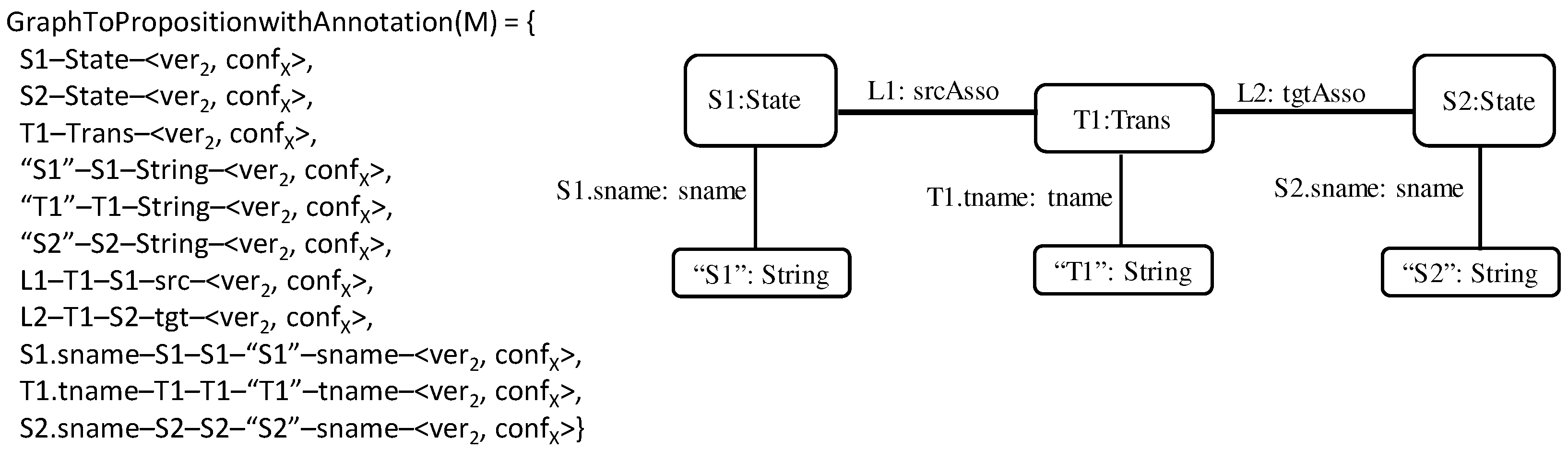
For example, if model M in Figure 12 is the second version of an initial model, say, M₀, and represents configuration X, then the propositional encoding of state S1 in that model is S1–State–<ver₂, conf_X> and the propositional encoding of a node attribute edge S1.sname is S1.sname–S1–S1–“S1”–name–<ver₂, conf_X>.

It is important to emphasize here that model M could be a union model rather than an individual model. According to Definition 8, because a union model $M_U$ is a model, the propositional encoding rules discussed above should be applicable to M_U, with the exception that the annotations of M_U elements are expressed as full STAL annotations instead of single model annotations. This means that the four rules stated in Definition 9 preserve their syntax and semantics when applied to M_U, except that the annotation format changes from single ver_nums and single conf_info into ranges, sets, or lists of ver_num and lists of conf_info.

Based on Definition 9, we can now define the mapping of an entire graph to propositions (with annotations), as follows:

Definition 10.

GraphToPropositionWithAnnotation: Given a typed graph G, a mapping of G’s elements into a set of propositions is GraphToPropositionWithAnnotation(G) = {ElementToPropositionWithAnnotation(elem)|elem ∈ N_G ∪ N_D ∪ E_G ∪ E_NA ∪ EEA}.

For example, the propositional encoding of the model in Figure 12 (repeated here for convenience) is shown to the left of Figure 13. We assume that the model here represents the second version of a given initial model and represents configuration X; that is, each of its elements is annotated with <ver₂, conf_X>.

5.2. Union of Propositional Encodings of Models

Given the propositional encoding of models discussed in the previous section, the union operation simply becomes the union of the propositional encodings of individual models, as follows:

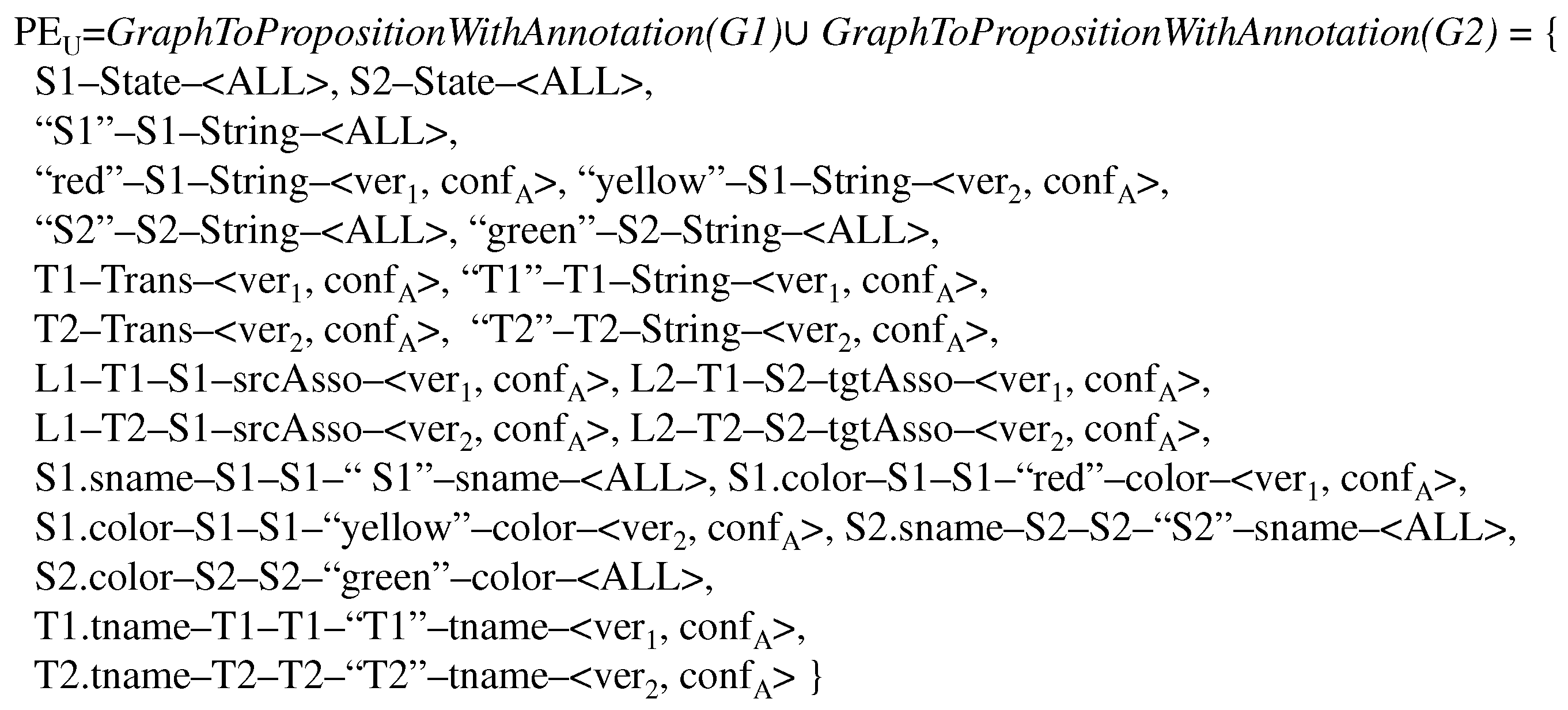
Definition 11.

Proposition Encoding Union (PE_U): Let MF be a model family of two models G1 and G2 (Definition 8), where G1 and G2 are attributed typed graphs with the same metamodel ATG, and let GraphToPropositionWithAnnotation(G1) and GraphToPropositionWithAnnotation(G2) be their propositional encodings (Definition 10); then, the union of the propositional encodings with annotations G1 and G2 is: PE_U = GraphToPropositionWithAnnotation(G1) ∪ GraphToPropositionWithAnnotation(G2).

We can generalize the above definition to a set of arbitrary encoded models, where the union of the propositionally encoded models is annotated according to the grammar of STAL following the approach in Section 4. Furthermore, because the union operation is incremental, a proposition encoding union (PE_U) can be unified with other individual models or even with other PE_Us. For instance, given a PE_U of a set of propositionally encoded models and a new model M_i encoded as GraphToPropositionWithAnnotation(M_i), their union becomes PE_{Unew =} PE_U ∪ PE_Mi. The annotations of PE_U and M_i are unified according to STAL.

5.3. Example

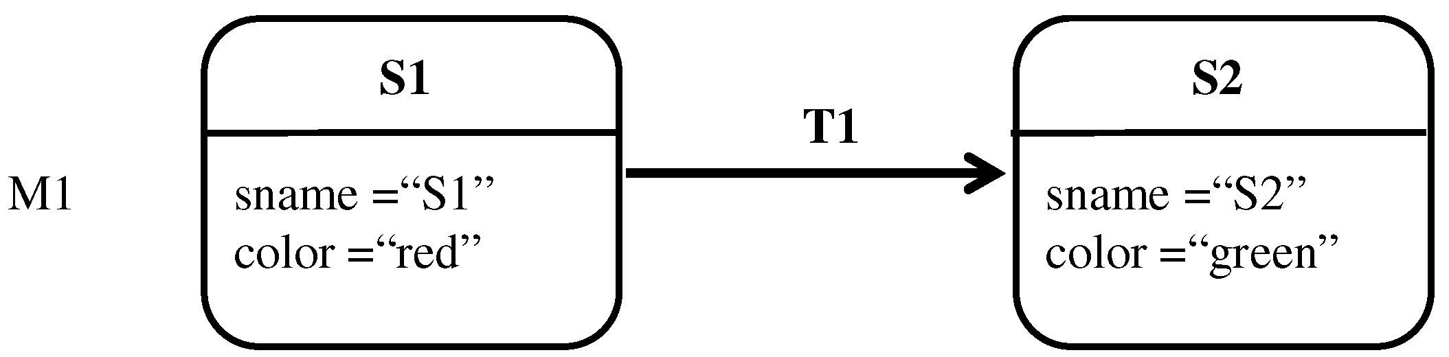
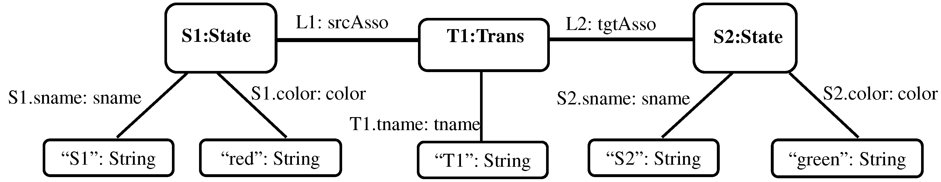
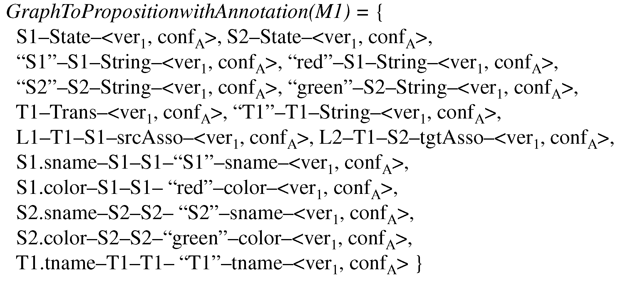
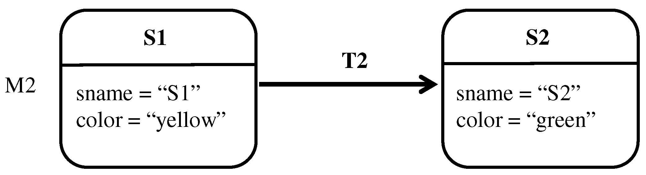
This section provides a simple yet complete example for two versions of state transition diagrams, M1 and M2. The example illustrates the formalization of both models as E-graphs. In addition, it illustrates their encoding into propositional variables as well as their union. In this example, M1 and M2 are assumed to be the first and the second version of a model that together represent configuration A. Hence, the elements of M1 and M2 are respectively annotated with <ver₁, conf_A> and <ver₂, conf_A>.

Figure 14 represents M1 in the conventional representation of state transition diagrams, Figure 15 illustrates the representation of M1 as a canonical typed attributed E-graph, and Figure 16 represents M1’s propositional encoding.

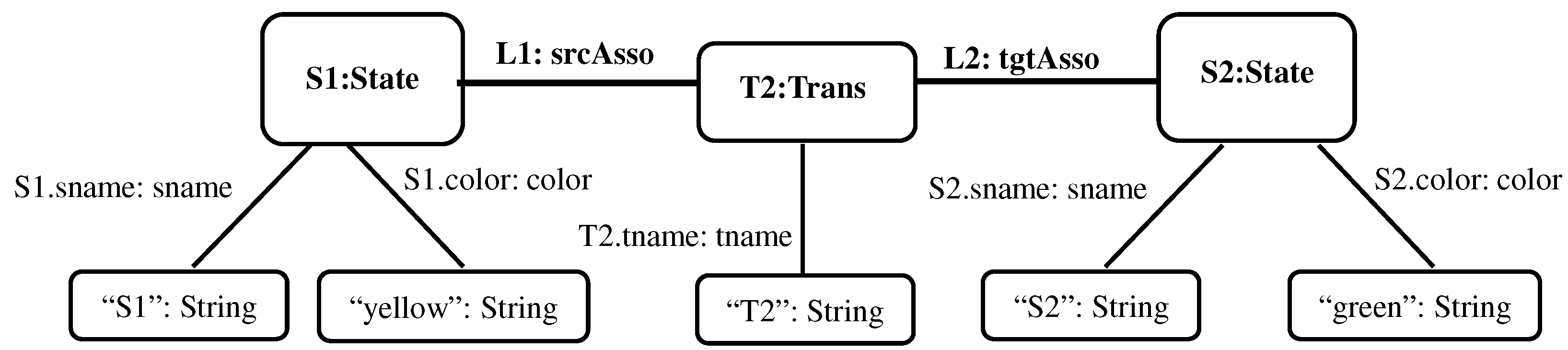
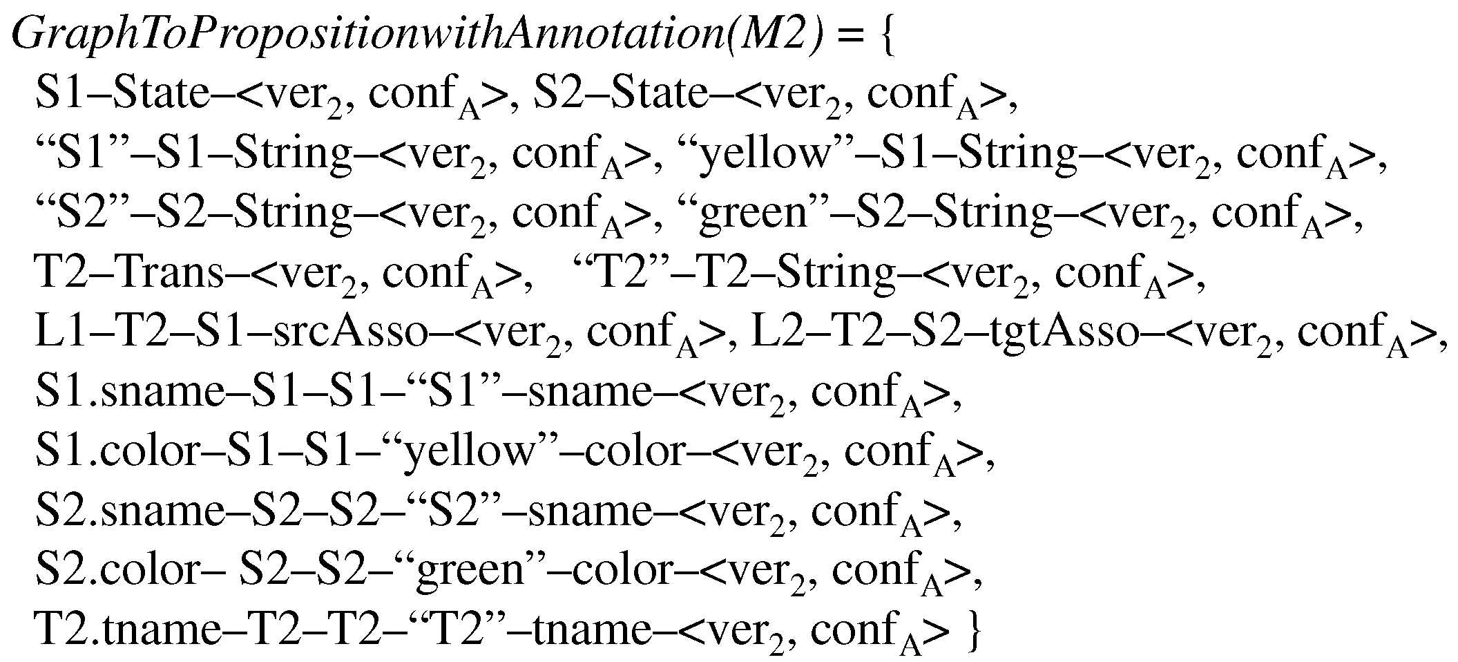
In the same manner, Figure 17 shows the conventional representation of M2 as a state transition diagram, Figure 18 represents it as an E-graph, and Figure 19 details its propositional encoding.

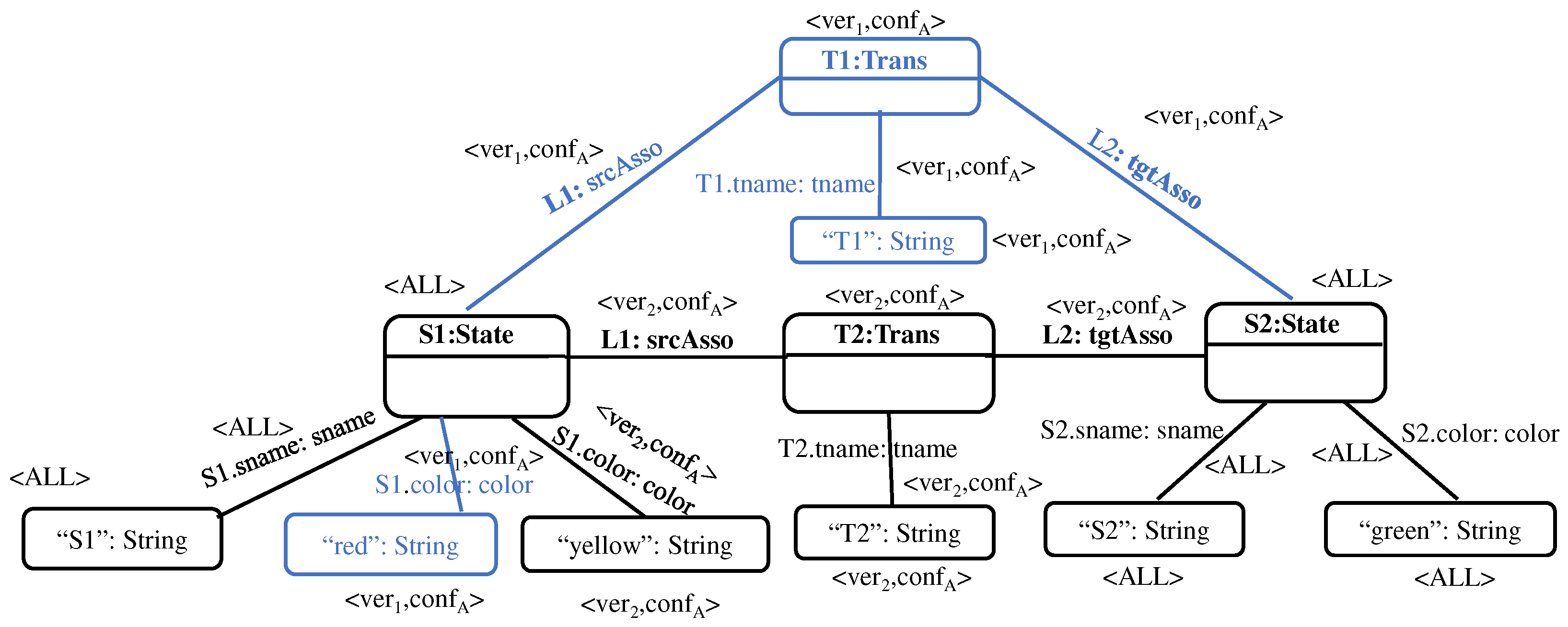
After encoding M1 and M2, we can now construct their union model $M_U$ as the union of their propositional encodings with annotations (Definition 11), as shown in Figure 20:

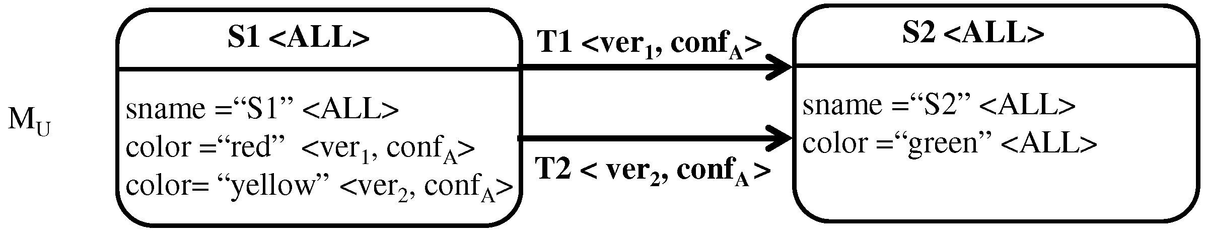
The representation of the union model as an E-graph is depicted (with annotations) in Figure 21, and its conventional representation as an ordinary state transition diagram (again with annotations) is shown Figure 22.

6. Analysis and Reasoning with Model Families

This section explores the research question: How efficient is reasoning and analysis with a group of models all at once using $M_U$ in comparison to the use of individual models?

To this end, Section 6.1 defines three reasoning tasks in order to evaluate their performance, first using union models and then using individual model several times. Section 6.2 discusses our experimental setup, methodology, and implementation. The next chapter then presents our results. A preliminary version of this section and the next one has previously been published in [12].

6.1. Reasoning Tasks

To answer the research question mentioned above, we need to describe how a union model can facilitate analysis and reasoning with sets of models instead of only single models. To achieve this, we consider three reasoning tasks (RTs), namely, property checking, trend analysis, and commonality analysis. Then, we compare the performance of the three RTs using $M_U$ as opposed to using individual models.

Although these kinds of analyses can be performed using individual models several times, one model at a time, our objective here is to make these analyses more efficient using $M_U$. In addition, we aim to reduce the effort needed for loading each model into a tool, analyzing the model, saving the analysis results, and then moving to the next model, especially as this effort cannot be neglected with a large number of models. These manual steps are, however, not considered in our results; as such, our results and performance improvements are conservative.

6.1.1. RT1: Property Checking

Property checking of models aims to verify whether or not a model satisfies a particular property. Given a model m and a property p, the result of property checking is either True if m satisfies p or False otherwise. For instance, a modeler may want to check whether or not a group of state machine diagrams contains self-looping edges, or she may check whether there exist two or more different actors in a GRL model family that contain the same goal. In these scenarios, property checking is beneficial to help modelers understand, for example, what is common between model versions or variations that violate a property.

In this section, we limit ourselves to language-independent syntactic properties (which describe the structure of models) other than semantic properties (which describe the behavior of models, e.g., traces). The rationale behind this scoping is because our approach aims to be applicable to any metamodel-based modeling language. However, while there exists a standard approach for defining the syntax of a modeling language (i.e., through metamodeling), there is no common approach for specifying semantics. Thus, we limit our approach to checking those properties related to a language syntax independently from any language specificity. Hence, “property” here means “syntactic property”. Alwidian [10] further discusses and evaluates semantic aspects for one particular language.

To perform property checking, we assume that a property p (expressed in any constraint language such as FOL or OCL) can be grounded over the vocabulary of models. Hence, a corresponding propositional formula $\mathsf{\Phi }p$ can be obtained. For example, given a well-formedness constraint $\mathsf{\Phi }p=\{\forall t:\mathit{Transition},\exists s:\mathit{State}|t.src=s\}$, it can be grounded over the vocabulary of the model in Figure 23 as follows:

As can be noticed, the example considers the graphical representation of the state machine presented in the canonical form in Figure 6b, where transitions T1 and T2 are represented here as directed edges between states and not as nodes.

Formally speaking, given the propositional encoding of both models (Section 5) and properties, the task of property checking can be defined as follows:

Definition 12.

Property Checking: Given a model m, property p, and their respective propositional encodings $\mathsf{\Phi }m$ and $\mathsf{\Phi }p$, we check whether the expression $\mathsf{\Phi }m\wedge \mathsf{\Phi }p$ is satisfiable or not using a SAT solver.

For RT1, inspired by van der Straeten et al. [23], we checked the “cyclic composition property”, which ensures that “the model does not contain self-looping edges”, i.e., $\mathsf{\Phi }p=\{\forall e:E_G,{\mathit{src}}_G\left(e\right)\ne {\mathit{tgt}}_G\left(e\right)\}$. It is important to highlight here that checking the self-looping edge property in individual models and in their $M_U$ is a simple reasoning task that always produces the same result; that is, if a self-looping edge exists in any of the individual models, then it will be detected in the $M_U$ that captures these individual models, and vice versa. This case, however, is not necessarily true for other properties, such as for example the general acyclicity property.

Figure 24 shows two simple state machine models that are acyclic (i.e., cycle-free) along with their union model $M_U$ that is not acyclic (i.e., has a cycle). In this scenario, checking the acyclicity property in individual models M1 and M2 produces a different result than checking the same property in $M_U$. To address this issue, there is a need to explicitly consider annotations on elements during property checking to determine the actual occurrence of cycles. For instance, if the link in model M1 is annotated with <v₁> and the link in M2 is annotated with <v₂>, then both links in $M_U$ will be considered as different and not as an actual cycle, even though they seem to constitute a structural cycle. A real cycle only exists when the intersection of the annotations of the links involved is not empty.

In the presence of annotations, property checking is more complicated and further research is needed to investigate its complexity. That is, we need to characterize the conditions under which this kind of property checking is beneficial when using $M_U$ in comparison to using individual models multiple times. The findings of Famelis et al. [6] regarding the analysis of syntactic properties of partial models indicate that the size of the model family might be an important factor; in smaller model families, it is better to analyze each individual model separately. In the future we want to investigate whether other factors, such as the degree of redundancy across the family or the shape of the models and property expressions, might play a role. In addition, counterexamples produced by model-checkers for union models that would violate a property would be harder to interpret than usual, as they might cover multiple models in the family. How to interpret such counterexamples in terms of individual models is left for future work.

6.1.2. RT2: Trend Analysis

This analysis aims to search for a particular element across members of a model family and to study the trend of that element, i.e., the behavior of elements over space/time. In other words, a trend analysis studies how properties of elements change over the course of time or across configurations. For instance, a modeler may need to search for a particular goal, say, GoalX, in all members of a GRL family in order to conduct a trend analysis about the properties of that goal (e.g., its importance/satisfaction value) and to observe how that value changes across model versions/variations in order to obtain insights into its evolution pattern.

6.1.3. RT3: Commonality Analysis

We suggest this type of analysis to enable modelers to check for those elements that are common in all (or part) of versions or variations of models in a family. This type of analysis is aligned with the commonality-based analysis in the SPL domain, where commonality is a key metric that indicates the reuse ratio of a feature across the SPL [24]. Following the same rationale, in this analysis it can be inferred that elements found to be common among the majority of models are important. For example, if a modeler is investigating several design options of a particular system and needs to know which elements are important in design options, then she would conduct this analysis once using the $M_U$ of the model family she has at hand instead of carrying out a pairwise search on each version/variation of individual models. To be fair, such analysis obviously needs to take into consideration the construction time of the union model.

6.2. Analysis and Experiments

We assessed the feasibility of reasoning using $M_U$ empirically by running experiments with parameterized random inputs that simulated different settings of various reasoning and analysis categories. In this chapter, we build on the formalization of union models in Section 3.3 and use formalized GRL models and state machine models. Our approach, however, is not bound to these languages, and is applicable to other metamodel-based languages.

6.2.1. Methodology

To evaluate the feasibility of using $M_U$ with the three reasoning tasks RT1, RT2, and RT3, we first measured the total time (in seconds) needed to perform each one of the RTs on each individual model one model at a time; we refer to this time as T_ind. Next, we measured the time needed to accomplish the same task with $M_U$; we refer to this time as T_MU. Then, we computed the performance improvements using the time metrics speedup (as used by Famelis in [25], defined originally as speedup = T_ind/T_MU) and time saving (in minutes for RT1 and in seconds for RT2 and RT3, calculated as TimeSaving = (T_ind − T_MU)).

Here, we define T_construct as the time needed to construct $M_U$. Although T_construct is usually quite small and can be performed once before being amortized over multiple analyses, we distinguish two categories of experiments, named Exp.1 and Exp.2. In Exp.1, we consider T_construct, such that the speedup is calculated as speedup_with_constrTime=T_ind/(T_construct + T_MU). In Exp.2, on the other hand, we neglect the time needed to construct $M_U$, where the speedup is calculated here (same as in [25]) as speedup_without_constrTime = T_ind/T_MU. In both experiments, a speedup larger than 1 is a positive result, and the larger the speedup, the better the improvement.

The reason why T_construct is considered here is to be more fair and realistic in the experiments, especially for large models, where it becomes necessary to not neglect the time needed to construct M_U. Another reason is to compare the results of both categories of experiments in order to reach a conclusion on whether or not to always neglect T_construct. As mentioned, the time that an analyst would need to analyze models individually in a realistic context by loading the model in a tool, performing the analysis, and saving the results is not taken into consideration in T_ind.

For both experiments, we considered the following experimental parameters: (1) the size of individual models (SIZE), which represents the number of elements (i.e., nodes and edges) in each individual model, and (2) the number of individual models in a model family (INDV). To control the possible combinations of parameters SIZE and INDV and to facilitate reporting, we followed the methodology proposed by Famelis et al. [6,25] to discretize the parameters’ domain into categories, where the ranges of values for the INDV parameter were set based on pilot experiments conducted by Famelis et al. [6] to determine reasonable ranges of individual models that constitute a family. Regarding the ranges of values for the SIZE parameter, we relied on our own experience with goal models, where models with a few dozen elements are considered to be small, while models with many hundreds or more elements are deemed to be extra-large.

For parameter SIZE, four categories were defined based on the number of nodes and edges, as follows: small (S), medium (M), large (L), and extra-large (XL). To calculate the ranges of each size category, we performed experiments with a seed sequence (0, 5, 10, 20, 40). The boundaries of each category were calculated from successive numbers of the seed sequence using the formula n × (n + 1). Using the same formula, a representative exemplar of each category is calculated by setting n to be the mean (rounded up) of two successive numbers in the seed sequence. We followed the same methodology for the number of individual models, INDV, using a seed sequence (0, 4, 8, 12, 16). The four size categories (S, M, L, XL) are shown in

Table 2. Categories of SIZE parameter (number of elements in a model).

#Elements/Model (SIZE)	(0, 30]	(30, 110]	(110, 420]	(420, 1640]
Exemplar	12	56	240	930
Category	S	M	L	XL

. The ranges of all categories of SIZE and INDV and the selected exemplars for each category are shown in

Table 3. Categories of INDV parameter (number of individual members in a family).

# of Indiv. Models (INDV)	(0, 20]	(20, 72]	(72, 156]	(156, 272]
Exemplar	6	42	110	210
Category	S	M	L	XL

. These ranges (generated from the seeds mentioned above) are in line with our own real experience dealing with goal models and state machines of various sizes. The same can be said for the number of individual models; a family is considered small when it contains a handful of models, and it is considered very large when it contains hundreds of models or more.

To evaluate the property checking task (i.e., RT1), each annotated individual model m in a model family $\mathit{MF}$ was encoded as a propositional logic formula, namely, $\mathsf{\Phi }m=\bigwedge \mathit{ElementToPropositionWithAnnotation}\left(e_i\right),e_i\in m$, where $e_i$ are elements of the model m. A union model $M_U$ of that MF was encoded as $\mathsf{\Phi }{M}_U=\bigwedge \mathit{ElementToPropositionWithAnnotation}\left(e_i\right),e_i\in M_U$. Furthermore, the property to be checked was encoded into a propositional formula $\mathsf{\Phi }p$. Afterwards, an SAT solver was used to check whether or not the encodings of each of the individual model and their union model satisfied the property. In particular, a formula $\mathsf{\Phi }m\wedge \mathsf{\Phi }p$ was constructed for each individual model. The property was said to hold in any model if and only if this formula was satisfiable. Similarly, a formula $\mathsf{\Phi }{M}_U\wedge \mathsf{\Phi }p$ was constructed and checked against whether the property was satisfiable. In both experiments, using the same computer settings, the time it took to check a property on individual models (T_ind) was recorded and compared to the time needed to carry out the check on union models (T_MU).

6.2.2. Implementation

To validate our approach, we used the NetworkX 2.2 Python library [26] to implement attributed typed graphs (according to Definition 5); we implemented our own union algorithm on top of that library to construct $M_U$ (based on Definitions 9 and 11). NetworkX 2.2 is a Python package for the creation, manipulation, and study of the structure, dynamics, and functions of complex graphs [26]. It is enriched with a variety of features, from the support of graph data structures and algorithms to analysis measures to visualization options.

To ensure that we had a family of state machine models, NetworkX’s graph generator was applied to randomly generate valid attributed typed graphs with different SIZE and INDV parameters. These graphs corresponded to typed state machines with likely evolutions, i.e., a sequence of random but typical manipulations on state machine models that lead to different versions. A sample of the generated graphs was manually checked to make sure that we had generated likely changes to existing models rather than generating completely independent models. Due to the completely random nature of the graph generators, we found that although the amount of changes in state machine models could be controlled, the topology of the resulting graph could not; that is, the same node in a model could change its incoming and/or outgoing edges randomly, leading to a different model. Such deviations between individual models can lead to a union model with large variations, indicated by the number of annotations on each element. Although this is not the best or even the typical case of state machine model families, we decided to perform experiments on the generated models in order to examine the complex families, for which the performance is unlikely to be worse.

For GRL models, the generation of models was less random; we took a set of real GRL models of smart homes published in [12] as a starting point and enlarged them according to the different combinations of the SIZE and INDV parameters. While growing the models, we created a set of random realistic modifications that involved adding and/or deleting intentional elements and/or element links or modifying their attributes. We then constructed G_U from the generated graphs using our union algorithm. G_U is the union of a set of typed graphs; hence, G_U corresponds to $M_U$.

It is worth mentioning here that the random generation of graphs was only used to check the scalability of the approach in order to provide a proof of concept for the suggested approach. Properties checked on such random graphs may be satisfied or not; this is not important here as long as the results for the model family are the same as the results for individual models, which is the case here.

For RT1, we checked the cyclic composition property inspired by [23], which ensures that the model does not contain self-looping edges. A propositional formula ($\mathsf{\Phi }p=\{\forall e:E_G,{\mathit{src}}_G\left(e\right)\ne {\mathit{tgt}}_G\left(e\right)\}$) was generated for this property. The propositional encodings were generated according to the rules discussed in Section 5, and were fed as literals to the MiniSAT solver included in the SATisPY package [27]. SATisPy is a Python library that provides an interface for various SAT solver applications.

To build confidence about the property checking results, the graphs and their union model were tested to check for the existence of any self-looping edges. Output solutions retrieved for individual models of a particular family were compared to the solutions returned for the corresponding union model. The results were the same. All experiments were executed on a laptop with an Intel Core i5-8250U (8th Gen) 1.6GHz quad-core CPU and 8 GB RAM running Windows $10\times 64$.

The next three sections are organized according to the experiments conducted to evaluate RT1, RT2, and RT3. All figures illustrated below represent a summary of the average results of fifteen runs represented for all SIZE and INDV categories together.

7. Results and Discussion

The results of the three reasoning tasks defined earlier are reported in Section 7.1, Section 7.2 and Section 7.3. Section 7.4 highlights the potential threats to validity. Finally, Section 7.5 provides a summary and a discussion of important points related to the current results and means of improving them in the future.

7.1. Results for Property Checking (RT1)

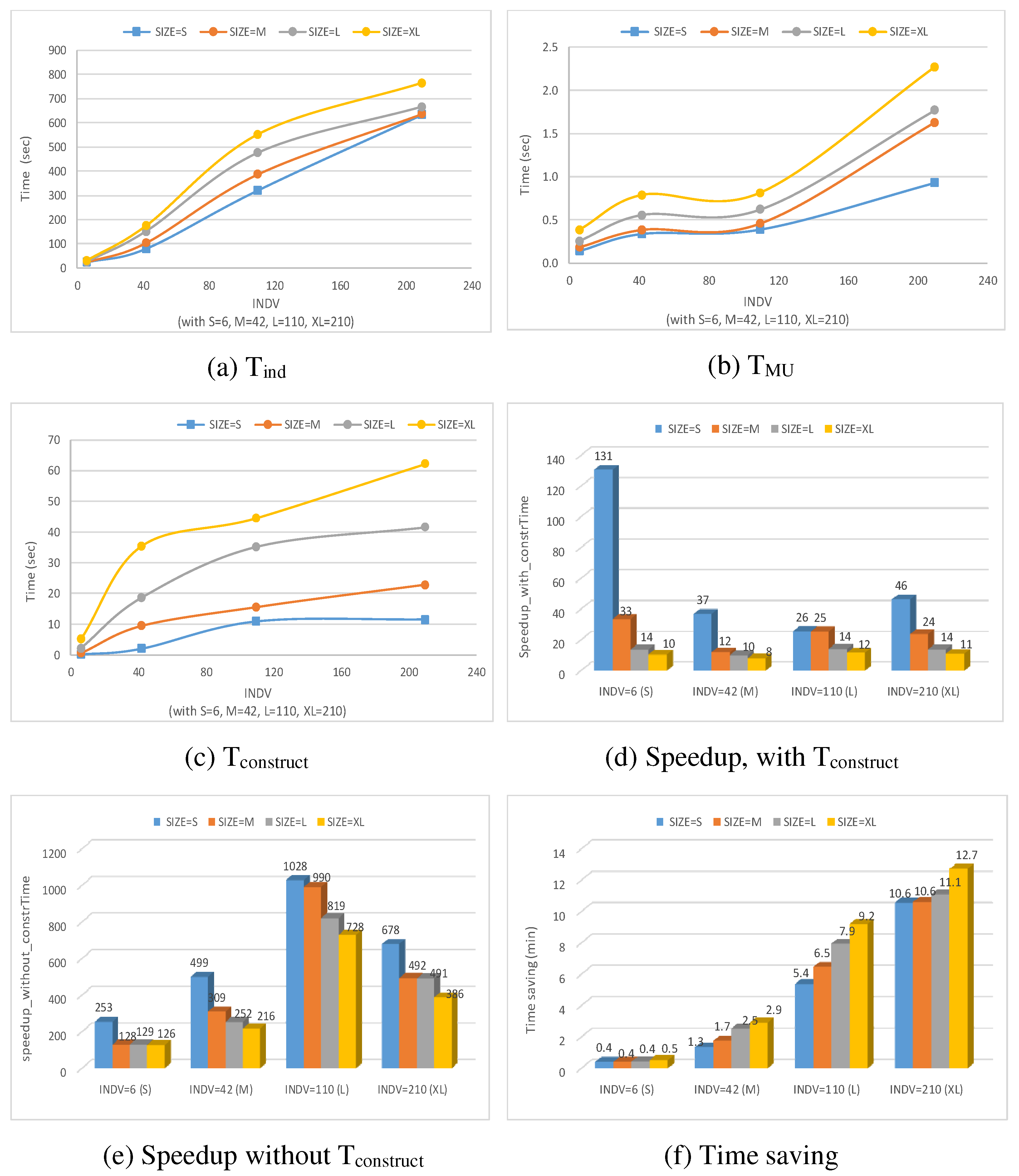
This section reports on our empirical results for the property checking reasoning task. Figure 25a illustrates T_ind, which is the total time performing property checking on each individual model, for all SIZE and INDV categories. Figure 25b reports on T_MU, which is the time needed to perform property checking on union models that capture individual models of different SIZE and INDV. In addition, Figure 25c shows the time T_construct needed to construct these union models. Figure 25d shows the time speedup with T_construct, i.e., speedup_with_constrTime = T_ind /(T_construct + T_MU), while Figure 25e shows the speedup without considering T_construct, calculated as speedup_without_constrTime = T_ind/T_MU. Finally, Figure 25f highlights the time saving in minutes achieved by using $M_U$ to perform property checking calculated as TimeSaving = (T_ind − T_MU).

Figure 25a–c shows that T_ind, T_MU, and T_construct increase when the size of models (i.e., SIZE) or the number of models in a family (i.e., INDV) increase. In addition, it can be noticed that the increase of T_ind is important for each SIZE category, as the INDV parameter grows from INDV = S to INDV = XL. For instance, with SIZE = XL, we observe 30.85 s on average for INDV = S to 765 s on average for INDV=XL. On the other hand, the increase of T_MU as INDV grows is marginal for each SIZE category. For example, for XL-sized models T_MU increases from 0.39 s (for INDV = S) to 2.25 s (for INDV = XL).

Furthermore, it can be inferred from Figure 25d,e that the use of $M_U$ for property checking achieves a noticeable time speedup compared to performing the same task on a set of individual models separately. For speedup_with_constrTime (Figure 25d), the highest speedup (=131) was observed with a small number of individual models (i.e., INDV = S) that are of a small size (i.e., SIZE = S). The smallest speedup (=8) was observed when INDV = M and SIZE = XL. In addition, Figure 25d shows that there is a noticeable pattern of speedup degradation for each INDV category as the number of elements per individual model (i.e., SIZE) increases. This is due in part to the increase of T_construct as the SIZE increases. Nevertheless, the speedup never falls below 1, which means that even with very large models (with INDV = XL and SIZE = XL) the time to perform property checking on a group of such models (using $M_U$), considering the time to construct $M_U$, is better than performing property checking on all individual models. Figure 25e shows that the time speedup becomes more significant when T_construct is ignored, where the highest speedup_without_constrTim = 1028 is with models of SIZE = S and INDV = L. This high value of 1028, which is higher than the number of models in family (110), is caused in part because of a low denominator value with low resolution (e.g., 1028 = 308.4/0.3), as well as by the time taken by the Python environment to load before executing the code of each individual model, which is not negligible, particularly for small models.

It is important to emphasize here that the erratic behavior of the time speedup with and without T_construct across all categories of SIZE and INDV does not necessarily mean that one category is superior to the other. This is because speedup reflects the ratio between T_ind and T_MU (and T_construct in case of calculating speedup_with_constrTime), and could fluctuate because of different densities of variability in the models.

It is not necessary that the speedup with INDV = S should be always better than that of INDV = M, INDV = L, etc., or vice versa, as the topology of the models generated may influence efficiency and this aspect is not controlled in this experiment. To this end, the speedup metric is used in this paper to demonstrate the improvements achieved by using $M_U$ in general, without regarding of the particular behavior of this improvement.

The TimeSaving metric, however, can be relied on to observe the behavior of the time gained from using $M_U$ to perform a particular task as opposed to using individual models multiple times. Figure 25f clearly illustrates a consistent pattern of time savings that increases when SIZE and INDV increase, which is the result that we were hoping for.

7.2. Results for Trend Analysis (RT2)

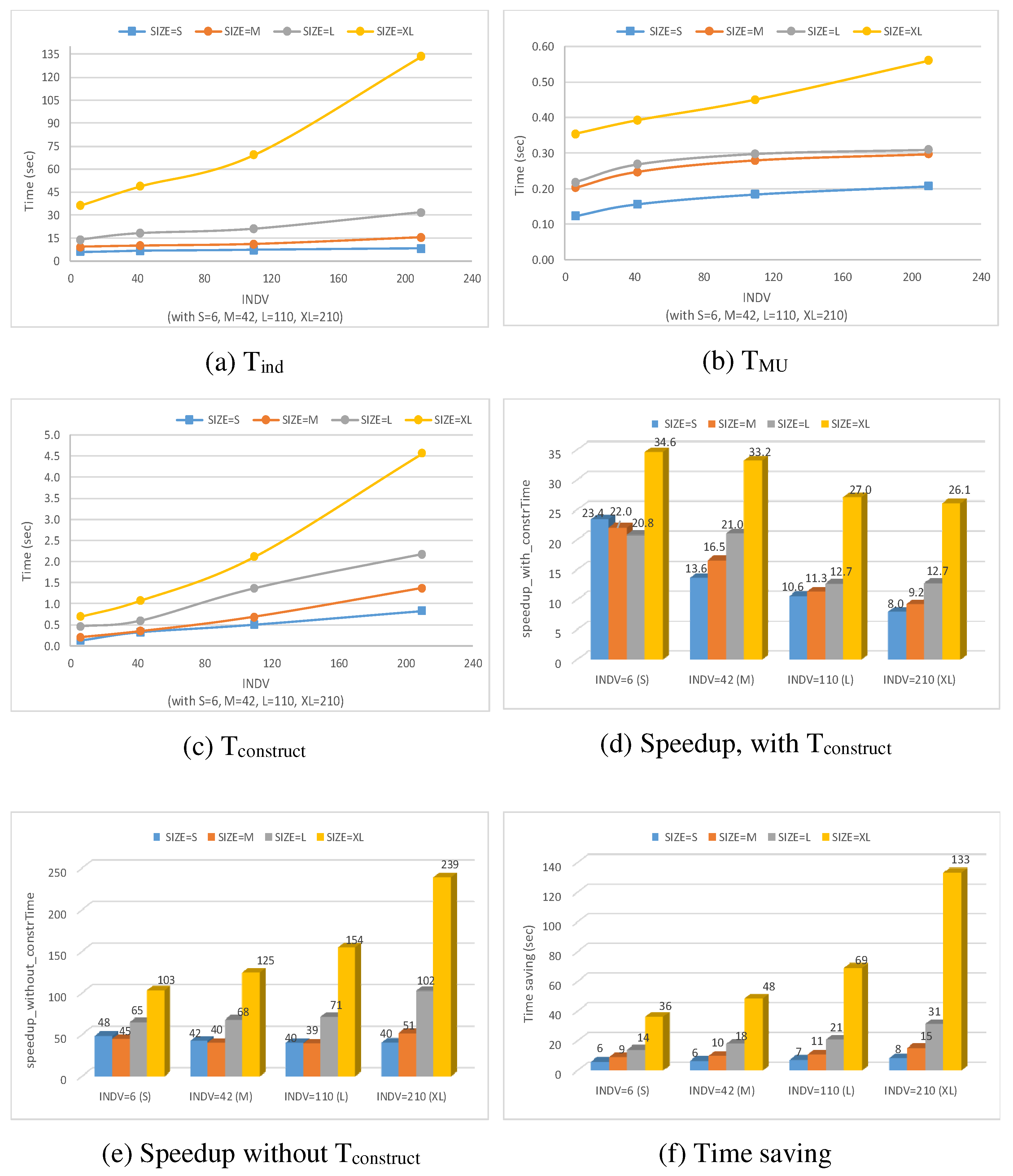
In this experiment, a trend analysis is conducted on an element named X-Goal from a set of individual GRL models and their union model $M_U$. The purpose of this analysis is to study the trend of this goal’s importance value attribute and analyze how this value changes over time. Performing this analysis on $M_U$ implies retrieving an element named X of type Goal, annotated with any version number <versions>, which could be a single version, a set of versions, or a range of versions that the element may belong to. With individual models, the search for and retrieval of X-Goal involve each individual model, where the laborious process in practice would involve opening each individual model, searching the desired element, observing its importance value, and closing the current model.

Figure 26a–c shows the respective T_ind, T_MU, and T_construct utilised in this experiment, while Figure 26d–f illustrates the time speedups, with and without T_construct and the time saved. The results in Figure 26a–c clearly illustrate a linear increase of T_ind, T_MU, and T_construct as SIZE or INDV increases. This is to be expected, as the searching task, which is the core of trend analysis, has a linear time complexity.

From Figure 26d, it can be noticed that for one SIZE category, SIZE = XL, the speedup decreases with the increase of the number of individual models in a family, i.e., INDV. This decrease is mainly due to the consideration of T_construct while computing the speedup. Nevertheless, the achieved speedups with T_construct are very positive and important. Without considering T_construct the speedup becomes more substantial, with a generally increasing pattern as INDV or SIZE increases, as depicted in Figure 26e.

Finally, Figure 26f demonstrates that the use of $M_U$ reduces the time needed to search for elements that belong to a group of models compared to traversing each individual model separately. This is clearly illustrated by the time savings, which substantially increase when SIZE or INDV increases.

7.3. Results for Commonality Analysis (RT3)

Figure 27 shows the results of conducting commonality analysis on a set of GRL models and their $M_U$. This experiment required searching for all elements that are common between all model versions. This is a tedious task, especially when the number/size of models increases. Searching a set of M individual models with N elements each to find elements in common between all models has a complexity of $\mathcal{O}(M\times N^2)$. However, with $M_U$ we only use one model to search for elements in common, where the task here is to search for elements annotated with <ALL>.

It can be noticed from Figure 27a that T_ind in this experiment is at least two times larger than T_ind in the previous experiment (i.e., RT2). T_MU and T_construct, on the other hand, grow at the same pace. Again, times T_ind, T_MU, and T_construct increase as SIZE or INDV increases.

The time speedup achieved by using $M_U$ is always positive, regardless of whether or not T_construct is considered. Figure 27d illustrates that speedup_with_constrTime shows a pattern close to that in RT2, that is, for one SIZE category, e.g., SIZE = S or SIZE = M, the speedup decreases as INDV increases. On the other hand, speedup_without_constrTime is more substantial, and increases as INDV or SIZE increases, as shown in Figure 27e. Finally, the time savings in this experiment (Figure 27f) are more significant than in the experiments for RT2, as the potential gain here is quadratic rather than linear, with about 133 s saved for extra-large families of extra-large models.

7.4. Threats to Validity

One major threat to the validity of our empirical evaluation stems from relying on randomly generated inputs, both graphs and experimental parameters. This threat can be alleviated by using more realistic parameters, e.g., using real-world model families.

Another threat is related to the experimental parameters, where we used only SIZE and INDV. We recognize that we need to examine the impact of the variability of models on reasoning. For example, we could consider the number of different annotations per element to describe how similar or different the members are. The topology of the graphs (e.g., depth, number of linked nodes, etc.) could benefit from specific experiments. The complexity of a property to be checked might be another parameter to consider.

Our experiments need to be elaborated further for more complex properties and analysis types, some of which might not exploit the STAL annotations as the ones used here could, and should be compared to other approaches that handle variability in the time dimension alone for goal models, including the work of Aprajita et al. [28] and that of Grubb and Chechik [29]. Furthermore, the current validation covers two modeling language, goal models and state machines, and should be extended to other types that are more structural, e.g., class diagrams, or behavioral, e.g., process models. Finally, the usefulness of our approach needs to be assessed and demonstrated with more significant examples or real-world case studies and a better quantitative comparison with existing approaches where there are overlapping analysis functionalities.

7.5. Summary and Discussion

Thus far, this paper has explored a research question related to the performance of union models by empirically evaluating the efficiency of reasoning and analysis tasks for modeling families using union models in comparison to the use of individual models. We defined three general reasoning tasks and evaluated their performance, first using union models and then using individual models several times. We have discussed the experimental methodology, setup, and implementation and reported on the empirical results. Our experiments demonstrate the usefulness and performance gains of union models for analyzing a family of models all at once compared to individual models. Finally, we have identified several threats to validity as caveats.

The speedups, whether the time for constructing the union model is considered or not, are always in favor of the union model, and these speedups generally increase as models or families grow larger. However, there is erratic behavior regarding the increase of the time speedup. For instance, the speedup for L-sized models in certain experiments was larger than the speedup of M-sized models, while in other experiments it was smaller than that for M-sized models. This behavior is due in part to the possibility of having a footprint for the creation of $M_U$, which is not negligible. Moreover, in order for the behavior of the speedup to be more stable and less erratic, we may need to consider additional experimental parameters such as the ratio of variability across models and the topology of the models at hand.

In addition, it is worthwhile to mention here that in certain individual experiments related to the calculation of speedup_with_constrTime we encountered counter-intuitive results, specifically, where the speedup was less than one. In such experiments, a speedup value less than one suggests that the use of $M_U$, when taking its construction time into account, is slower than the use of individual models. Again, these slowdowns where obtained in individual experiments only, and they were amortized by calculating the average results of fifteen runs.

In terms of concrete time saved, which ranges from half a second to a few minutes depending on the experiment, the savings may not seem large at first glance; however, there are several practical implications:

• The time savings accumulate as many analyses are performed on a same union model, especially as the union model construction time is amortized over multiple analyses;
• The savings doe not take into account the concrete time required when a practitioner uses a tool to open a model, perform the analysis, and save the results, which this may take many seconds per model and is prone to human error;
• The savings become essential in a context where union model construction and verification are offered as a service, i.e., as an online application where multiple users can concurrently upload, merge, and analyze their model families.

While this paper focuses on analysis types that are language independent, the first author’s previous work in [10,30] explored the adaptation or lifting of language-dependent analyses for a given language, namely, forward and backward propagation of satisfaction values for GRL model families, again with positive performance gains. The GRL-based analysis algorithms and their lifted version were implemented using an optimizer (IBM CPLEX) with speedups up to 23 times faster when using the union model compared to individual models, and for a much lower additional memory cost. In practical terms, this means that analysis on model families is no longer limited to the verification of behavioral properties often seen in existing approaches.

In addition, while conducting property checking our focus was not on the type of properties to be checked (i.e., semantic vs. syntactic properties); rather, the focus was on examining the improvement of performance in terms of time speedup for performing any kind of property checking (syntactic in this paper) when using union models once as compared to performing the same task using many models in the model family one model at a time. In the future, it would be possible to differentiate between the types of properties to be checked and assess the impact of the property type on the overall performance of the analysis.

8. Related Work

In the literature, few approaches have been proposed to support model families. Shamsaei et al. [9] used GRL to define a generic goal model family for various types of organizations in the legal compliance domain. They annotated models with information about organization types to specify which were applicable to which family members. Different from our work, the work of [9] handled only variation of models in the space dimension, and did not consider evolution over time. In addition, the authors focused only on maintainability issues and did not propose union models to improve analysis complexity and reduce analysis effort. Palmieri et al. [8] elaborated further on the work of [9] to support more variable regulations. The authors integrated GRL and feature models to handle regulatory goal model families as software product lines (SPLs) by annotating a goal model with propositional formula related to features in a feature model. Unlike [9], Palmieri et al. considered further dimensions such as the organization size, type, the number of people, etc. However, they did not consider the evolution of goal models over time, and did not introduce union models.

Our work has strong conceptual resemblances with the domain of SPL engineering, which aims to manage software variants in order to efficiently handle families of software [31,32]. The notion of a feature is central to variability modeling in SPL [33], where features are expressed as variability points. Feature models (FMs) [16] are a formalism commonly used to model variability in terms of optional, mandatory, and exclusive features organized in a rooted hierarchy and associated with constraints over features. FMs can be encoded as propositional formula defined over a set of Boolean variables, with each variable corresponding to a feature. FMs are deemed to be very useful to represent feature dependencies, describe precisely allowed variability between products in a product line, and guide feature selection to allow for the construction of specific products [34,35]. However, it is important to emphasize here that FM is different from our proposed union models $M_U$ in both usage and formalism. The differences between both artifacts can be summarized as follows:

• A feature model represents variability at an abstract “feature level”, which is separate from software artifacts (such a grammar of possible configurations), whereas $M_U$ represents the variability of all existing models at the “artifact level” itself [36];
• While a feature model defines all possible valid configurations of products along with constraints on their possible configurations, an $M_U$ provides a complete view of the solution space that makes it explicit for modelers which particular element belongs to which model without necessarily modeling dependencies or constraints between elements of one model or across several models of a family;
• The purpose behind using both artifacts is different, in that FMs are mainly used to ensure that the derived individual models are valid through valid feature configurations, with the possibility of generating new models or products. On the other hand, $M_U$ is proposed to perform domain-specific analysis beyond configuration validation more efficiently on a group of existing models than on individual models;
• Finally, an $M_U$ enables the extraction of individual members of a model family by means of selecting particular time and/or space annotations, while FM enables model extraction by means of selecting valid combination of dependency rules and cross-tree constraints between features.

There exist verification approaches that target many valid configurations of feature models [37]. For instance, Classen et al. [38] explored the use of model checking on a family of behavioral models captured by a feature model, with resulting gains in verification time. Similar approaches have been developed for real-time SPLs [39], for symbolic model checking [40], and for probabilistic model checking [41], among others [42]. These approaches are, however, limited to the space dimension (no evolution of models over time) and to behavioral properties, e.g., they cannot be used to reason about satisfaction propagation in a family of goal models, which is allowed by the usage of $M_U$ [30].

To express variability, annotative approaches are commonly used in the literature, such as in the work of Czarnecki and Antkiewicz [34], in which variability points are represented as presence conditions. These conditions are propositional expressions over features. Annotations of features can be used as inputs to a variability realization mechanism in order to derive or create a concrete software system as variant of the SPL. Using a negative variability mechanism, annotative approaches define a so-called 150% model that superimposes all possible variations for the entire SPL. The 150% model is used to derive a particular variant, while other irrelevant parts are removed. While union models have similarities to 150% models, the uses of both models, the domains they are used in, and the ways of annotating them are all different.

Ananieva et al. [43,44,45] proposed an approach for consistent view-based management of variability in space and time. In particular, the authors studied and identified concepts and operations of approaches and tools dealing with variability in space and time. Furthermore, the authors identified consistency preservation challenges related to view-based evolution of variable systems composed of heterogeneous artifacts and provided a technique for (semi-)automated detection and repair of variability-related inconsistencies.

Mahmood et al. [46] presented an empirical assessment of annotative and compositional variability mechanisms for three popular types of models, namely, class diagrams, state machine diagrams, and activity diagrams. The authors provided recommendations to language and tools developers and discussed findings from a family of three experiments with 164 participants in total, in which they studied the impact of different variability mechanisms during model comprehension tasks. The authors recommended that annotative techniques lead to better developer performance and noted that the use of the compositional techniques correlates with impaired performance. In addition, for all the experiments it was found that annotative variability is preferred over compositional variability by a majority of the participants for all task types and in all model types.

The approaches proposed by Seidl et al. [14], Ananieva et al. [47], Michelon et al. [48,49], and Lity et al. [15] are closely related to ours. In the context of SPL engineering, they considered variation of software families in both space and time, and explicitly annotated variability models with time and space information to distinguish between the different versions and variations of software artifacts.

Different from approaches for managing the variability and evolution, Wittler et al. [50] have introduced a variability model for both software and hardware that captures variability in both space and time as well as the dependencies between loosely coupled software and hardware components. The authors refined the Unified Conceptual Model by introducing system generations to reflect the implicit dependencies between software and hardware components in product lines.

Even though the concept of a “family” is shared between our work and the SPL domain, the main difference is one of purpose and scope. At its core, SPL engineering is a software engineering methodology for systematic proactive reusability. The overarching concern is to strategically design, plan, and maintain a set of software artifacts according to points of functionality (features). Then, by exploiting commonalities between variants, engineers can efficiently derive or create software products with desirable features. It is not the goal of our work to plan for reusability or to derive new models or products. Characteristically, union models do not depend on modeling common functionalities in a feature model. Such a model is expressly created to facilitate proactive reusability, and is a central concept in SPLs.

Instead, we use union models to analyze families of existing models irrespective of their provenance or the intent for which they were constructed. As an object-oriented technology, union models generalize SPLs by decoupling family modeling from the particularities and exigencies of proactive reusability. Union models are a step towards a more basic and fundamental idea: the representation and analysis of families of models.

Famelis et al. [6] proposed partial models to capture a set of possible alternative models with design-time uncertainty. The emphasis of this work was to create a methodology for the lifecycle of design-time uncertainty. This includes articulating modelers’ uncertainty about design decisions, maintaining this uncertainty, and supporting systematic decision-making via refinement [51]. Dhaouadi et al. [52] addressed the challenges of design-time uncertainty by proposing DRUIDE (Design and Requirements Uncertainty Integrated Development Environment), a language and workflow for articulating design time uncertainty. DRUIDE provides modelers with the ability to explicitly articulate uncertainty and compose completely heterogeneous models by linking uncertainties. This work is related to decision-oriented Product Line Engineering (PLE) [53], mainly as design uncertainty often involves modeling sets of design alternatives. Furthermore, DRUIDE is related to research on creating representations of sets of related models, which is in turn related to our work on model families. Compared to the work of Famelis et al. [6] and Dhaouadi et al. [52], the focus of our work is more fundamental, looking at efficient reasoning about model families by leveraging redundancies across members of the family. Naturally, the three approaches are complementary, and we are actively researching various synergies.

The use of a single model to represent multiple interrelated systems was proposed by Stünkel et al. [54]. Similar to our approach, they used typed graphs to represent commonalities between models. The authors focused on interoperability, consistency specification, and consistency restoration, and did not consider the representation of modeling families or variability representation in space and time.

Aprajita et al. [28,55] extended the GRL metamodel to document explicit changes (additions/deletions) of elements to specific versions of a model. Although a model family can be captured, this approach is specific to one language and is currently incomplete in terms of the kinds of changes to versions that it can accommodate.

Grubb et al. [56,57] introduced the concept of dynamic intentions into goal models to capture alternatives on multiple time scales. The authors proposed a tool-supported method for specifying changes in intention over time which uses simulations to ask a variety of “what-if” questions about models that evolve over time.

Hablutzel et al. [58] investigated the problem of model merging for Tropos goal models. In particular, the authors proposed a formal approach to address the problem of automatically merging the attributes of intentions and actors in which both static models and models with timing information were considered. In their work, Hablutzel et al. looked at the initial creation of a goal model through merging, rather than tracking model evolution over space and time through a merged representation using union models.

9. Conclusions and Future Work

In this paper, we propose union models as a first-class generic artifact to capture and represent model families. The paper provides a graph theory-based formalization of model families and their union models. In particular, model families are formalized as a set of attributed typed graphs in which all models are typed over the same metamodel. Metamodels are formalized as attributed type graphs, whereas union models are formalized as the union of all graph elements in the set of typed attributed graphs which constitute a model family. Included in the union model are the graph elements annotated by the models they are occurring. The purpose of this formalization is to permit representation of model families and their union models independent of any modeling language used in the context of MBSE. In addition, we propose a Spatio-Temporal Annotation Language (STAL) to support the representation of variability in model families in both the space and time dimensions and to facilitate reasoning about union models.

We demonstrate how the properties of these formalisms can be used to support the construction of union models as well as to perform typical reasoning tasks, such as trend analysis and property checking, on union models. We empirically illustrate the potential of using union models to improve analysis and reasoning over a set of models all at once as opposed to analyzing single models separately one at a time. Positive results are observed even when the time taken to construct union models is taken into consideration; in practice, the construction time can be amortized over many analyses.

The artifacts related to this paper are available online. These include Excel files for attributed typed graphs defined according to the formalization provided in Section 3. In addition, GRL model families generated for four SIZE categories (i.e., small, medium, large, X-large) for our experiments, and the Python programs used for the union algorithm, for generating models, and for measuring the reasoning tasks defined in Section 6 are included. See https://bit.ly/UnionModelsExtra, accessed on 8 February 2023.

For future work, there are many opportunities to follow up on several directions:

• Studying the effects of variation and topology on reasoning techniques: it is necessary to describe how sensitive reasoning and analysis are to the degree of variation in a union model, as well as where this variation is located (topology). The degree of variation of an $M_U$ can be inferred from the number of annotations and the number of annotated elements that exist in a model family and are represented by that $M_U$.
• Improved tool support: although a prototype tool exists for creating union models, the software ecosystem could be greatly enhanced by providing conversion from metamodels (in EMF or MOF) to type graphs and from models to typed graphs expressed with PELA. Tools to better visualize annotated union models in the original language’s syntax whenever possible would be very useful. Support for more rigorous lifting analysis methods and editors would contribute to the practical adoption of the proposed approach.
• Studying the usability of the approach: there is a need to assess which practitioners this approach is useful to and which parts require usability enhancements in order to improve adoption in industry, especially regarding automation. We envision offering merging and several types of reasoning as online services.
• Exploration of further synergies with techniques for representing and managing design-time uncertainty using partial models [51]. Specifically, we would like to adapt model transformation lifting to union models and to develop operators for managing union models across their lifecycle.