Ant-Balanced Multiple Traveling Salesmen: ACO-BmTSP

Abstract

A new algorithm based on the ant colony optimization (ACO) method for the multiple traveling salesman problem (mTSP) is presented and defined as ACO-BmTSP. This paper addresses the problem of solving the mTSP while considering several salesmen and keeping both the total travel cost at the minimum and the tours balanced. Eleven different problems with several variants were analyzed to validate the method. The 20 variants considered three to twenty salesmen regarding 11 to 783 cities. The results were compared with best-known solutions (BKSs) in the literature. Computational experiments showed that a total of eight final results were better than those of the BKSs, and the others were quite promising, showing that with few adaptations, it will be possible to obtain better results than those of the BKSs. Although the ACO metaheuristic does not guarantee that the best solution will be found, it is essential in problems with non-deterministic polynomial time complexity resolution or when used as an initial bound solution in an integer programming formulation. Computational experiments on a wide range of benchmark problems within an acceptable time limit showed that compared with four existing algorithms, the proposed algorithm presented better results for several problems than the other algorithms did.

1. Introduction

In recent years, intelligent computation technologies have received increasing attention from researchers. Most of these technologies are inspired by natural phenomena and attempt to use the virtues of elements of behavior. A technique for problem solving inspired by the behavior of ants when finding paths from their nest to food sources (ant colony optimization—ACO) gained special importance due to its successful results when applied to optimization problems [1,2]. The original ACO underwent several modifications in order to adapt it to different real-world problems, such as assignment problems, graph coloring, scheduling, circuit design, communication networks, bioinformatics, vehicle routing, etc. Several ACO extensions have been created since then, such as elitist AS [3], Ant-Q [4], Ant Colony System [5], rank-based AS [6], population-based ACO [7], Beam-ACO [8], etc. Later, the ACO algorithm was combined with other algorithms to create denominated hybrid methods and to obtain better results. Some examples of hybrid methods using ACO are found in [9,10,11,12,13,14,15,16,17,18].

When the traveling salesman problem (TSP) is extended to consider multiple salesmen (mTSP), other kinds of algorithms can use this technique to solve more general problems. Some works focused on solving the mTSP are reviewed in the following. Harrath et al. [19] proposed a hybrid algorithm, AC2OptGA, for solving the mTSP. The algorithm used genetic (GA), ant colony, and two-opt algorithms. The ant colony algorithm was used to generate solutions, and the two-opt algorithm and GA were used to enhance the solutions that were obtained. These algorithms used instances for $n=\{51,100,150\}$ and $m=\{3,5,10\}$. Gomes et al. [20] implemented a GA in a vehicle-routing problem (VRP). The goal was to optimize daily routes for workers assigned to distribution for a company located in a city (Covilhã, Portugal). They claimed to reduce the total distance traveled by 618 km per week in comparison with the company runs. They considered $n=270$ nodes, three zones, and a five-day window. The primary goal was to minimize the cost and distance instead of balancing the tours. The cost-balanced TSP is one of the recent variants of the TSP. Thus, Akbay and Kalayci [21] proposed a solution based on the variable neighborhood search algorithm to solve the cost-balanced TSP. They used twenty-two datasets, which included small-, medium-, and large-scale instances, to obtain computational results. Muñoz-Herrera and Suchan [22] focused their research on fitness landscape analysis (FLA) for the multiple traveling salesman problem (mTSP) and capacitated VRP (CVRP). They proposed a new FLA measure that provided valuable information for characterizing the fitness landscape’s structure under specific scenarios and obtained several relationships between the fitness landscape’s structure and algorithmic performance. Garn [23] developed a balanced dynamic closest vehicle heuristic (BD-CVH) and a balanced dynamic assignment vehicle heuristic (BD-AVH) to solve a dynamic routing problem for the balanced mTSP. The obtained distances indicated that, in general, the BD-AVH algorithm led to slightly better solutions. Xu and Zhang [24] implemented a hybrid algorithm for the balanced mTSP based on genetic algorithms and the two-opt algorithm. Khoufi et al. [25] proposed a review of the existing literature devoted to UAV (unmanned aerial vehicle) path optimization problems related to two existing general classic problems, the traveling salesman problem and the vehicle-routing problem. They provided a synthetic overview of the resolution techniques and performance metrics, and they obtained numerical results. Pereira et al. [18] proposed a hybrid method, GACO2, for solving the mTSP based on the genetic algorithm, ant colony optimization, and the two-opt algorithm to improve the solution. They applied this method in two instances—mTSP51 and mTSP100—with 3, 5, and 10 travelers. The primary purpose was to find the minimum distance traveled by using the minisum number of salesmen. Pereira et al. [26] implemented a hybrid algorithm, GABC-LS, to solve the minisum mTSP based on a genetic algorithm, an artificial bee colony, and two local search methods (move1-within and two-opt). This was a small-sized instance.

Table 1. Advantages and drawbacks of the reviewed approaches.

Approach	Advantages	Drawbacks
ACO	– Rapid discovery of good solutions	– Premature convergence
[1]	– Efficient in solving the TSP	– Falls easily into the trap of local optima
		– Does not guarantee the optimal solution
AC2OptGA	– Efficient with medium- and large-sized instances	– Does not guarantee the optimal solution
[19]	– Probability of a fall into local minima minimized	– Highly time-consuming
GA to m-TSP	– Reduction of 618 km per week	– Does not guarantee the optimal solution
[20]	– Huge impact in several forms	– Highly time-consuming
	– Contributions to fostering smart cities
FLA for mTSP	– Efficient exploration of the solutions of features of spaces	– Generally impossible to draw a fitness landscape with a huge search space
[22]	– Provides relevant information about optimization method improvement	– Generally impossible to draw a fitness landscape with a huge search neighborhoods
	– Gets relationships between the FL structure and the algorithmic performance
BD-mTSP	– Predicts travel distance based on dynamic parameters	– Solution is not immediately provided
[23]		– Leads to slightly better solutions
GACO2	– Efficient in solving small-sized mTSP instances	– Does not provide balanced tours
[18]	– Allows the release of traveling salesmen	– Not tested on large-sized instances
GABC-LS	– Efficient in solving small-sized mTSP instances	– Does not provide balanced tours
[26]	– Uses only one method	– Highly time-consuming

indicates the pros and cons of the reviewed algorithms. Considering balanced tours, most works used the minimax function. Therefore, the minimization of the maximum tour value may neglect variations in smaller tours. This phenomenon implies a loss of the algorithm’s sensibility and compromises the feedback clues that the optimization function gives to the search. On the other hand, combining ant and other optimization algorithms in a hierarchical structure leads to a long computation time. Keeping these ideas in mind, the following research questions were formulated:

• Is it possible to solve the mTSP by using optimization functions without dead zones?
• Could the mTSP be solved by using ant colony optimization with minor modifications?

This paper proposes a novel algorithm based on ACO for the mTSP with several depots. The main contributions are the following: (i) an innovative objective function that enables simultaneous achievement of two goals—minimal distance and balanced tours; (ii) a refined version of ACO that includes a proposal for an ant-picket algorithm instead of an ant finding a complete path alone, and the solution is subdivided into several tours to be searched by a group (picket) of ants. For the experimental assessment in this proposal, a group of instances proposed by Carter and Ragsdale [27], by [28], and by [29] were used to validate the proposed algorithm.

This paper is organized as follows: The multiple traveling salesman problem used in the experimental study is presented in Section 2.1. Section 2 presents the ACO algorithm and associated concepts, describes the application of ACO to the mTSP, and presents the proposed approach. Section 3 presents the simulation results. Section 4 discusses the advantages of the proposed algorithm. Finally, the main conclusions and suggestions for future studies are presented in Section 5.

2. Methodology

This section begins by describing the basics of the mTSP. Next, Section 2.2 describes the ACO algorithm, Section 2.3 explains how ACO can be used in the mTSP, and Section 2.4 presents the proposed approach to solving the mTSP to obtain balanced tours.

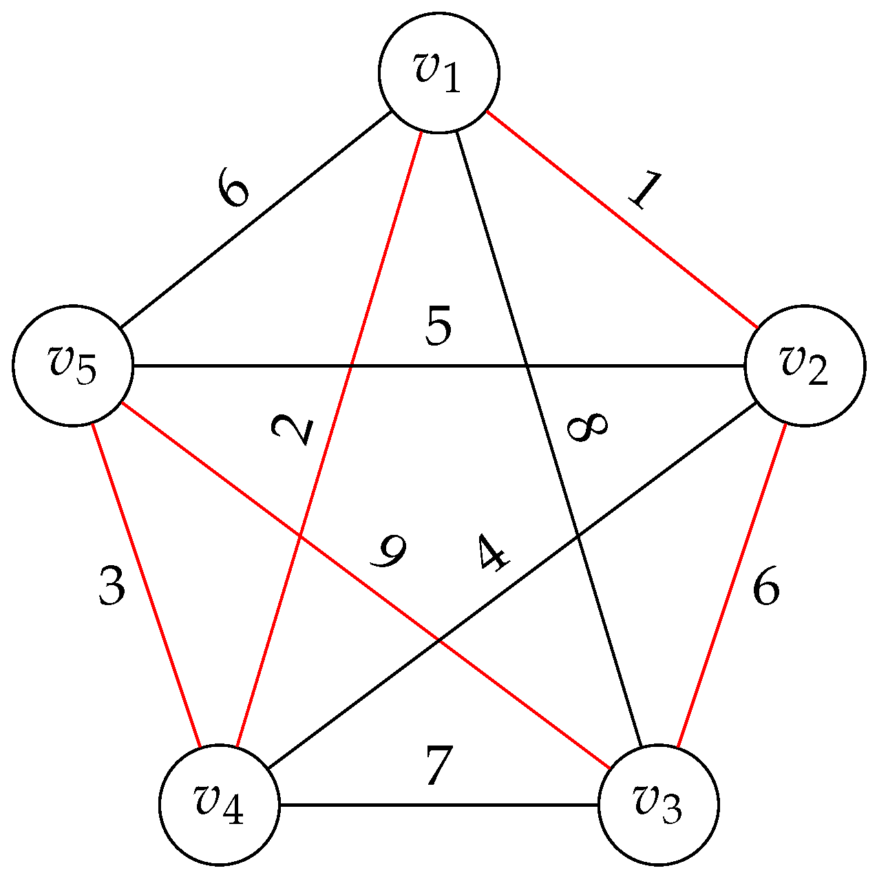
2.1. Basics of the Multiple Travel Salesman Problem

One of the best-known classic combinatorial problems is the traveling salesman problem, or the TSP for short [30]. According to [31], the TSP was studied in the eighteenth century by two mathematicians, William Rowam Hamilton and Thomas Penynington Kirkman. The TSP has the objective of minimizing a value—usually the distance—while defining a sequence of locations, where each is visited exactly once by a salesman, who then returns to the starting city. The travel can be described as a graph $G=(V,E)$ with a set of n vertices V connected by m edges E, where $V=\{v_1,v_2,...,v_n\}$ and $E=\{e_1,e_2,...,e_m\}$. In this graph, the vertices represent the cities and the edges represent the roads or possible paths to go from one city to another, with an associated cost value. To be able to take a trip that passes through all of the graph vertices of the graph only once constitutes, in graph theory, the so-called Hamiltonian circuit. Considering the vertex $v_1$ as the depot, in Figure 1, the Hamiltonian circuit has an associated cost of 21. This cost can have a different meaning depending on the problem and can be evaluated with an objective function.

The graph in Figure 1 shows five vertices $V=\{v_1,v_2,v_3,v_4,v_5\}$, each one representing a city, interconnected by edges. The paths taken from one vertex to another have an associated cost represented by the number near the line. The simplest way to solve the TSP is to try all possibilities by using exhaustive methods, but when the number of edges grows, those methods are too time-consuming and computationally expensive. On the other hand, exact methods are useful when they solve problems within a reasonable time, e.g., in the production–inventory–routing problem [32], in discrete truss topology design [33], and in wind farm layout problems [34]. Due to the TSP’s time complexity, when the number of cities becomes high, heuristic and metaheuristic methods are used to solve the problem. Heuristics do not guarantee that the optimal solution to the problem is found, but they can return a quality solution in an adequate amount of time for several application needs. A heuristic’s main purpose is to find a good solution simply and quickly. On the other hand, metaheuristics are models that serve as a guide for building heuristics. Many of those models are based on natural phenomena. The TSP has many different real-world applications, such as school bus routing, management of pickup and delivery, and others [35], making it a prevalent problem to solve. However, some problems require additional salesmen. Thus, the multiple TSP (mTSP) is defined to generalize the usual TSP. This generalization uses more than one salesman to find a solution. It can be defined as a set of n nodes and m salesmen initially located at a single depot node. All salesmen start and return to the depot, and all remaining cities are visited only once by a unique salesman [36].

To model the single-depot mTSP precisely, assuming that the problem is symmetrical, that is, $c_{ij}=c_{ji}$, the equations are:

$$min\sum _{j=1}^n\sum _{i=1}^n{c}_{ij}{x}_{ij}$$

(1)

$$\sum _{j=1}^n{x}_{1j}=\sum _{j=1}^n{x}_{j1}=m$$

(2)

$$\sum _{j=2}^n{x}_{ij}=1,i=1,2,\dots ,n$$

(3)

$$\sum _{i=2}^n{x}_{ij}=1,j=1,2,\dots ,n$$

(4)

$$u_i-u_j+n{x}_{ij}\le n-1,2\le i\ne j\le n$$

(5)

$$x_{ij}\in \left\{0,1\right\},i,j=1,2,\dots ,n$$

(6)

The objective function is described by (1), with the goal of minimizing the total associated cost, which is subjected to several constraints. Constraint (2) ensures that exactly m traveling salesmen start and return to the initial depot (vertex 1). Restrictions (3) and (4) ensure that exactly one edge enters and exits each graph city. The sub-tour elimination constraint (5) defines an integer variable $u_i$ for the position of node i in a tour, and n represents the maximum number of nodes visited by any salesman. Finally, (6) defines the variable $x_{ij}$ as binary.

The mTSP is more appropriate than the TSP for many practical applications, and it can be used to simulate many real-life applications [37], e.g., disaster management, cooperative missions, monitoring and surveillance, transportation and delivery, multi-robot task allocation and scheduling, WSN data collection network connectivity, search and rescue, and precision agriculture, among others [37]. Many variants of the mTSP have been reported in the related literature. The most important for this study is the understanding of the variant classification according to the objective function; two main formulations of the mTSP exist [37]:

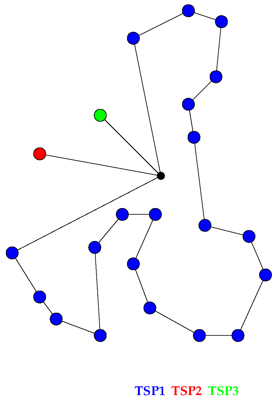
• MiniMax mTSP: In this mTSP variant, the objective function consists of minimizing the most extended tour cost among the tours of all salesmen.
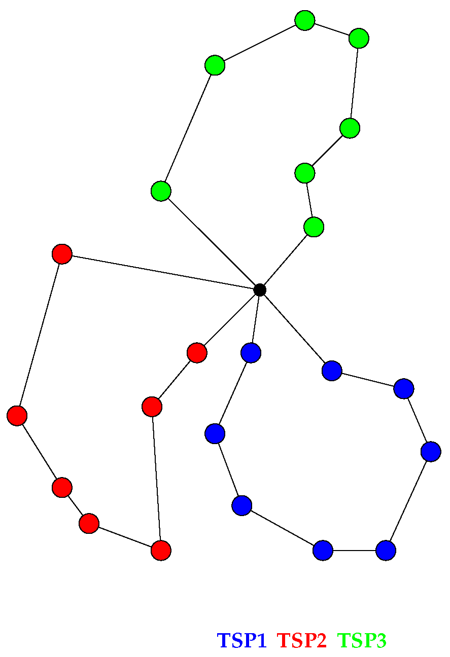
• MiniSum mTSP: In this mTSP variant, the objective function consists of minimizing the sum of the tour costs of all salesmen.

Although a majority of reported works about the mTSP sought to minimize the total distance traveled by all the salesmen (minisum), minimizing the maximum distance traveled by any salesman (minimax) is of more practical significance, since it is related to balancing the workload among salesmen [38].

2.2. The ACO Algorithm

This section briefly presents the ACO metaheuristic, which belongs to a bio-inspired class of optimization algorithms. The ACO algorithm proposed by Marco Dorigo [39] is inspired by real ants’ behavior in nature. Ants’ communication takes place through the secretion of a semiochemical and odorous substance called a pheromone to guide the direct food path from the destination to the source [40]. To search for food sources, ants go out and realize a path, dropping a certain amount of pheromones on the ground. Pheromone initialization is the most critical step, and the initialized quantity of pheromones is equivalent for all graph nodes [40]. The edge pheromone amount, ${\tau }_{ij}$, between edges i and j is evaluated according to the following formula:

$${\tau }_{ij}=(1-\rho ){\tau }_{ij}+\sum _{k=1}^{n_{\mathrm{a}}}\Delta {\tau }_{ij}^k$$

(7)

where $\rho$ is the pheromone evaporation rate, $n_{\mathrm{a}}$ is the number of ants that visited the edge $(i,j)$, and $\Delta {\tau }_{ij}^k$ is the amount of pheromone deposited by ant k in the edge $(i,j)$. This amount of pheromone is calculated with:

$$\Delta {}_{ij}^k=\left\{\begin{array}{cc}Q/L_k,\hfill & iftheantkhaspassedthroughthisedge\hfill \\ 0,\hfill & otherwise\hfill \end{array}\right.$$

(8)

where $L_k$ measures the path distance visited by ant k, and Q is a constant value. After the ants have passed a particular edge of the graph, they need to choose the next edge to follow in order to reach the food source. The amount of pheromone in the next edge to choose will be decisive, so the greater this amount is, the greater the probability will be that the ant will select the corresponding edge. The probability of movement of ant k from node i to node j, which has not been visited yet, is calculated with:

$$p_{ij}^k=\frac{{\left[{\tau }_{ij}\right]}^{\alpha }{\left[{\eta }_{ij}\right]}^{\beta }}{{\sum }_{l\in N_i^k}{\left[{\tau }_{ij}\right]}^{\alpha }{\left[{\eta }_{ij}\right]}^{\beta }}$$

(9)

where $\alpha$ is a parameter that represents the importance of the edge pheromone in deciding the subsequent movement of the ant; $\beta$ is a parameter that represents the importance of the distance in deciding the subsequent movement of the ant; $N_i^k$ is a set of nodes that have not yet been visited by ant k; ${\eta }_{ij}$ is the inverse distance between nodes i and j. A cycle is completed when all ants have finished their movement. As time goes by, it turns out that ants will tend to follow the shortest path, thus tending to converge to the problem’s optimal solution.

The ACO algorithm can be described step by step, as presented in Algorithm 1.

Algorithm 1 ACO Algorithm.

1: Initialize parameters 2: Position ants at starting node 3: while stop condition is not satisfied do 4:     Ants build a solution 5:     Update pheromone 6:     Local search (optional) 7:     Update best solution 8: end while 9: Save best solution

2.3. Applying ACO to the BmTSP

As real ants are able to find the shortest path between a food source and their nest without using visual mechanisms, but only by exploiting a trail of pheromones, they can be similarly applied to the mTSP, considering the nest as a single depot and the location of a food source as the location of other cities. The road network in the mTSP was modeled with a graph simulating the path traveled by real ants to find food. Figure 2 and Figure 3 show an example of three salesmen traveling to twenty-three cities while using two different variants: the minisum and unbalanced work (Figure 2)—where only the total cost (in this case, the distance) was the aim considered—and the minimax (Figure 3)—where the work was more balanced, but the only goal to minimize the path with the maximum salesman cost.

Most reported studies focused on solving the mTSP by using a minisum formulation, and only very few aimed to specifically minimize the maximum distance traveled by all of the salesmen [41]. However, the best solutions showed that the salesmen’s paths were not equitable or balanced. A small percentage of salesmen traveled most of the paths, while the rest traveled very short distances. To try to eliminate this disadvantage, this study focused on an attempt to achieve a single function that consisted of a combination of the shortest total path (minisum) and a minimization of the maximum subpath (minimax) in order to obtain balanced paths for each salesman. The mTSP was called balanced (BmTSP) when each salesman visited approximately the same number of cities or had the same tour cost. Therefore, the BmTSP was used, and the equitable distribution of some types of resources was important. Some authors formulated this problem by minimizing the maximum tour values. In terms of optimization, this function presents some gaps. If the ‘lower’ tours—the tours with lower distance values—change, the objective value could remain the same. Therefore, this change is not reflected in the objective function and does not give any clues for driving the search in the right direction.

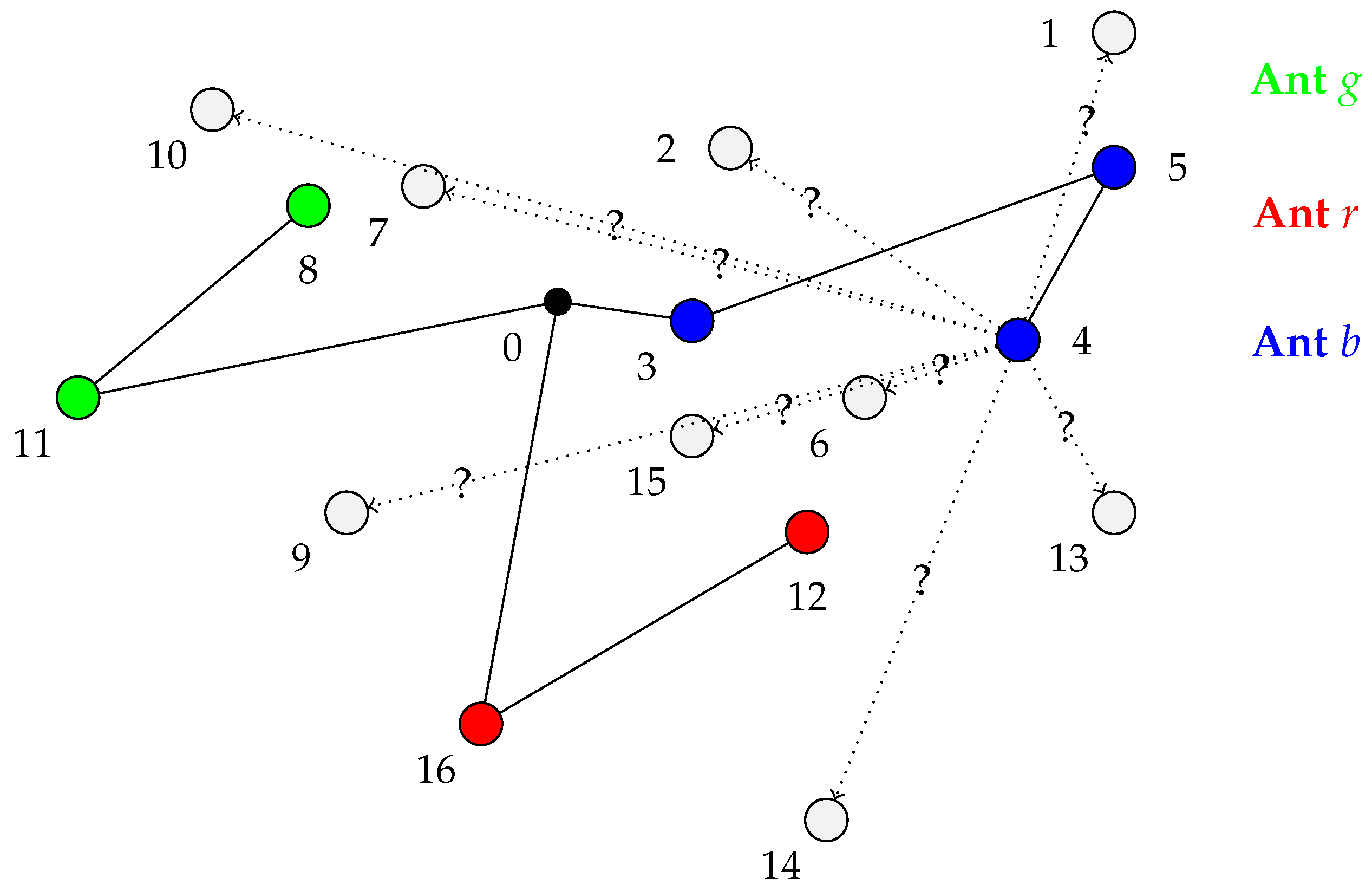
2.4. The Proposed Approach: ACO-BmTSP Algorithm

This work focuses on an implementation of ACO consisting of a substantial modification in its application. Instead of using an ant to create a tour, an ant picket is used in the proposed algorithm. This algorithm, ACO-BmTSP, replaces lines 4 and 5 of Algorithm 1.

The first step of this technique is to initialize all of the ACO parameters (line 1:3 of Algorithm 2; the cost of each ant is zero at the beginning, $c_j=0$; the ant picket begins at the deposit, $u_j=\left\{Deposit\right\}$, and the set of unpicked nodes includes all except the deposit). As the single-depot variant of the mTSP was used, all the ants of the picket were positioned in this city (by analogy, the initial graph node; line 2). Instead of considering only one ant, as in the classical single TSP, in this algorithm (ACO-BmTSP), a group of ants m was considered to obtain a solution. Each ant j stores a tour, in the set $u_j$, and all ants’ tours forms a potential solution of the problem. Therefore, in Algorithm 2, for each instance (a solution of the problem), the tours were built in the “while” loop as follows: The ant of the picket whose cost is minimum (line 5) selects an unpicked city based on the pheromone path (line 6); it updates its set of visited cities (line 7), the cost traveled according to the distance $d_{p_j{p}_i}$ between the last and current cities (line 8), and the global set of unpicked cities (line 9). The instance is finished when there is no city to pick, and the ants return to the deposit. The pheromone is spread as in the original ACO. Each solution created in an ant picket iteration is evaluated by using the objective function (10). This function minimizes the cost of the tours and promotes balanced tours. Since it is a continuous function, it suppresses the insensibility mentioned in the previous section, where each tour variation leads to a variation in the objective function. In this function, $S_j$ is a set of $|S_j|$ arcs traveled by the salesman k.

$$f=\sqrt{\sum _{k=1}^m{\left(\sum _{j=1}^{|S_j|}{c}_j\right)}^2},j\in S_j$$

(10)

Algorithm 2 Ant picket algorithm.

1: $c_j=0$, $\forall j\in \{1,2,\dots ,m\}$ 2: $u_j=\left\{Deposi{t}_j\right\}$, $\forall j\in \{1,2,\dots ,m\}$ 3: $P=\{1,2,\dots ,n\}\setminus \left\{Deposits\right\}$ 4: while$P\ne \varnothing$do 5:     Find the ant j with the lowest cost $c_j$ 6:     Select $p_i\in P$ according to the transition rules 7:     $u_j=u_j\cup p_i$ 8:     $c_j=c_j+d_{p_j{p}_i}$ 9:     $P=P\setminus \left\{p_i\right\}$ 10: end while 11: Return the tour solution

Minimizing function (10) leads to a solution with the minimum cost and balanced tours. Although this perception is evident concerning the minimum cost, obtaining balanced tours may not be straightforward. This intention becomes apparent if the following optimization problem is considered: Suppose that two salesmen have a route of 100 units to travel, and they want to divide the route so that each one travels the same path distance. This problem can be formulated to determine the distance each one travels as follows:

$$\begin{array}{c}\mathrm{Minimize}:\hfill \\ c_1^2+c_2^2\hfill \\ \mathrm{s}.\mathrm{t}.:\hfill \\ c_1+c_2=100.\hfill \end{array}$$

The solution of this problem is $c_1=c_2=50$. Thus, squaring the factors that each salesman travels leads to balanced tours. The same reasoning was successfully applied to minimize robotic manipulator trajectories and determine their “balanced” intermediate configurations [42,43].

Using integer programming formulation and the same deposit, this problem can be represented by Equations (11)–(16), where $x_{ij}^k$ is one if the arc $\left(ij\right)$ belongs to tour k, and zero otherwise. The square root of the objective function (11) could be eliminated, since the optimization result would be the same. $u_i^k$ is the position of node i in the tour k. The other variables have the same meanings as those used when considering Equations (1)–(6). Namely, m is the number of the TSP, n is the number of cities, and k is the number of tours.

Constraint (12) ensures that exactly m traveling salesmen start and return to the initial depot (vertex 1). Restrictions (13) and (14) ensure that exactly one edge enters and exits each graph city. The sub-tour elimination constraint (5) defines an integer variable $u_i$ for the position of node i in a tour, and n represents the maximum number of nodes visited by any salesman. Finally, (6) defines that the variable $x_{ij}$ is binary.

$$min\sqrt{\sum _{k=1}^m{\left(\sum _{j=1}^n\sum _{j=1}^n{c}_{ij}{x}_{ij}^k\right)}^2}$$

(11)

$$\sum _{k=1}^m\sum _{j=1}^n{x}_{1j}^k=\sum _{k=1}^m\sum _{j=1}^n{x}_{j1}^k=m$$

(12)

$$\sum _{k=1}^m\sum _{j=2}^n{x}_{ij}^k=1,i=1,2,\dots ,n$$

(13)

$$\sum _{k=1}^m\sum _{i=2}^n{x}_{ij}^k=1,j=1,2,\dots ,n$$

(14)

$$u_i^k-u_j^k+n{x}_{ij}^k\le n-1,2\le i\ne j\le n,k=1,2,\dots ,m$$

(15)

$$x_{ij}^k\in \left\{0,1\right\},i,j=1,2,\dots ,n,k=1,2,\dots ,m$$

(16)

Consider a problem with three traveling salesmen/ants, one deposit, and 16 cities. Figure 4 presents one state in which the ant-picket algorithm is used. In the following, it is explained how to reach this state with the three ants: {green (g), red (r), blue (b)}. The ants randomly select the next city to visit while taking the pheromones deposited in each arc into account. In the beginning, the ants $(g,r,b)$ are at the deposit. Therefore, the cost is $c=(0,0,0)$ and $u_g=\left\{0\right\},u_r=\left\{0\right\},u_b=\left\{0\right\}$. Suppose that the chosen cities are 11, 16, and 3 for ants g, r, and b, respectively, leading to $c=(25.49,22.36,\mathbf{7}.\mathbf{07})$, $u_g=\{0,11\},u_r=\{0,16\},u_b=\{0,3\}$. Since the ant b has the smallest distance cost, minimum distance traveled by an ant is flagged as boldface, it selects the next city—for example, city 5, reaching $c=(25.49,\mathbf{22}.\mathbf{36},30.48)$, $u_b=\{0,3,5\}$. Suppose that ant r selects city 12 ($c=(\mathbf{25}.\mathbf{49},42.08,30.48)$, $u_r=\{0,16,12\}$), g selects city 8 ($c=(41.09,42.08,\mathbf{30}.\mathbf{48})$, $u_g=\{0,11,8\}$), and b selects city 4 ($c=(41.09,42.08,\mathbf{40}.\mathbf{78})$, $u_b=\{0,3,5,4\}$). At this point, since the ant b has the lowest cost, it selects the next city considering only the unpicked cities $P=\{1,2,6,7,9,10,13,14,15\}$. Figure 4 illustrates this state. Circles or cities with colors: green, red, and blue were selected by the ant with the respective color. Additionally, the filled edges indicate the order of the visited cities. On the other hand, gray circles represent unpicked cities. In this stage, ant b at node 4 will select one of those cities. Dotted lines with a “?” highlight those possibilities. The algorithm continues until the set of all of the unpicked cities is empty, and the ants return to their deposit.

3. Experimental Results and Analysis

For each mTSP instance, the algorithm was run thirty times in order to verify the stability of the algorithm. The experimental results are shown in Section 3.2, and a comparison with other works is also shown in this section’s tables. To improve the understanding of the obtained values, some figures show the paths traveled by each salesman, indicating the cities with nodes and the paths taken between cities with lines connecting the cities. A set of instances contained a total of 11 instances. It is noted that all of the paths started and ended at the same node (depot). In the mTSP51 instance, the depot used was $(32,39)$, in the mTSP100 instance, the depot used was $(1819,814)$, and in the mTSP150 instance, the depot used was $(2310,236)$. For all of the remaining instances, the first city was set as the depot. There were five small instances called 11a, 11b, 12a, 12b, and 16. Instances 11a, 12a, and 16 comprised the first 11, 12, and 16 cities of mTSP51. Instances 11b, 12b, and 128 were derived from the sp11, uk12, and sgb128 datasets [44]. The mTSP instances with n = 51, 100, and 150, kroD100, and rat783 were based on the TSPLIB [45].

3.1. Parameters of the ACO Algorithm

The performance of metaheuristics such as the ACO algorithm directly depends on the choices of parameter values. As described in Section 2.2, the original ACO has few parameters to initialize: the pheromone evaporation rate, $\rho$, the number of ants running per iteration, $Ants$, the number of the best ants who deposit pheromones $Bests$, the exponent of the pheromones $\alpha$ (a higher value of alpha provides pheromones with more relevance), and, finally, $\beta$, the exponent of distance (a higher value of beta provides the distance with more weight). As usual, the choice made for each parameter value is based on the method’s efficiency. For both ACO algorithms, the parameter values were the same. The number of cycles performed until the stop condition was satisfied was 240 iterations. The number of ants used was 3200, and the number of ants that spread pheromones was 45. The remaining parameters used with their values were $\rho =0.05$, $\alpha =1$, and $\beta =1$.

3.2. Computational Results

In order to evaluate the proposed algorithm’s performance, several benchmark mTSP instances were tested. All of the experiments were performed on the Google Colab platform, which allowed code in the Python language to be run.

The instances used considered several numbers of cities and $m=\{3,5,10,15\}$ salesmen, leading to 19 different problems. Each instance was run, and the results are presented in

Table 2. Total and partial distance traveled by salesmen when using the ACO-BmTSP algorithm.

					TSP N.º (0, 1, 2, 3)
Name	m	Total	Avg.	Std.	1 + 5l	2 + 5l	3 + 5l	4 + 5l	5 + 5l
mTSP51	3	468.09	156.03	4.19	160.73	154.69	152.68	–	–
	5	523.78	104.75	7.41	117.36	105.00	101.91	100.92	98.58
	10	765.83	76.58	9.30	93.44	88.11	82.39	79.43	76.61
					74.41	70.36	68.39	66.64	66.06
mTSP100	3	24,455.04	8151.69	579.15	8580.49	8381.72	7492.87	–	–
	5	27,309.44	5461.89	311.23	5772.65	5664.10	5591.60	5255.97	5025.12
	10	43,824.70	4382.47	689.43	5264.51	5136.02	4942.60	4870.01	4508.78
					4148.68	4119.31	4086.25	3619.29	3129.26
mTSP150	3	39,471.09	13,157.03	76.97	13,211.62	13,190.47	13,069.00	–	–
	5	44,322.33	8864.47	146.69	9082.80	8922.60	8845.47	8763.26	8,708.21
	10	58,298.47	5829.85	508.42	6221.31	6188.45	6125.01	6103.19	5,974.78
					5957.49	5936.46	5700.35	5587.74	4503.69
11a	3	224.18	74.73	5.12	78.17	77.17	68.85	–	–
11b	3	265.09	88.36	10.80	96.31	92.71	76.07	–	–
12a	3	226.53	75.51	3.77	78.17	77.17	71.20	–	–
12b	3	3073.08	1024.36	108.56	1100.77	1072.21	900.10	–	–
16	3	271.79	90.60	4.38	93.89	92.28	85.62	–	–
mTSP128	10	47,256.11	4725.61	1268.96	6304.43	6247.17	6163.11	5954.47	3967.22
					3954.17	3904.04	3902.46	3765.28	3093.76
	15	75,394.28	5026.29	1187.69	6190.42	6143.34	6127.44	6020.33	5995.13
					5954.85	5886.04	5655.69	5006.01	5001.86
					3601.67	3600.24	3565.89	3382.81	3262.55
kroD100	3	26,009.03	8669.68	1077.89	9828.23	8484.31	7696.49	–	–
	5	32,808.35	6561.67	926.92	7929.75	6918.62	6528.11	5770.61	5661.26
	10	47,256.09	4725.61	1268.96	6304.43	6247.17	6163.11	5954.47	3967.22
					3954.16	3904.04	3902.46	3765.27	3093.76
rat783	20	25,089.70	1254.55	136.22	1413.45	1374.56	1365.69	1353.25	1347.03
					1345.72	1338.38	1322.84	1313.55	1303.64
					1299.97	1289.81	1276.78	1231.01	1221.94
					1201.95	1157.57	1023.50	1005.08	903.99

. Columns 1 and 2 indicate the numbers of cities and salesmen. Column 3 presents the total cost of each solution. In the next columns, Avg and Std present the average and standard deviation, respectively. The following five columns indicate each tour’s cost in descending order. The first five tours are in black in the line, and for the ten- and fifteen-salesman problems, the next five and last five are in gray in the second and third lines, respectively.

For the problem with 51 cities and three salesmen, a total cost of 468.09 and tour costs of $\{160.73,154.69,152.68\}$ were obtained. The tours had a difference of 8.05 between the maximum and the minimum cost, leading to an average of 156.03 and a standard deviation of 4.19. On the other hand, for $m=\{5,10\}$, an average and standard deviation of 104.75 and 76.58 were achieved, respectively. Considering the problem with 100 cities, the average costs obtained were $\{8151.69,5461.89,4382.47\}$ for 3, 5, and 10 salesmen, and the standard deviations obtained were $\{7.10\%,5.69\%,15.7\%\}$. Finally, for the mTSP150 problem, the average costs and standard deviations were {13,157.03, 8864.47, 5829.85} and {76.97, 146.69, 508.42} for 3, 5, and 10 salesmen, respectively. Considering the small-sized group of instances (11a, 11b, 12a, 12b, and 16, which were all for three salesmen), the average costs obtained were $\{74.73,88.36,75.51,1024.36,90.60\}$, and the standard deviations obtained were $\{5.12,10.80,3.77,108.56,4.38\}$, respectively. For the problem with 128 cities and ten salesmen, the average costs obtained were $\{4725.61,5026.29\}$, and the standard deviations obtained were $\{1268.96,1187.69\}$. For the instance kroD with 100 cities, the average costs were $\{8669.68,6561.67,4725.61\}$, and the standard deviations were $\{12.4\%,14.1\%,26.9\%,15.7\%\}$ for 3, 5, and 10 salesmen, respectively. Finally, for the rat783 instance, which considered 783 cities and 20 salesmen, the average costs were 1254.55, and the standard deviation was 136.22.

The results obtained enabled to conclude that salesmen’s paths were generally well balanced, and the difference in the distances was minor. The algorithm found balanced routes for all salesmen. Additionally, as the number of salesmen increased, the cost of individual tours decreased.

To perform the best interpretation of the results, Figure 5, Figure 6 and Figure 7 show the real paths traveled by each salesman for 51 cities. Each color identifies the cities visited by a salesman. Salesman 1 (TSP1) follows the path whose cities are represented by blue, TSP2 by red, and TSP3 by green. In problems with five and ten salesmen, TSP4 travels through pink cities and TSP5 through gray cities. Finally, in problems with ten salesmen, TSP6 travels by cities represented by yellow, TSP7 by maroon, TSP8 by dark gray, TSP9 by cyan, and TSP10 by magenta. It is possible to see the positions of all cities in the space and the path for each salesman. Figure 8, Figure 9 and Figure 10 show the real paths traveled by each salesman for 100 cities.

To compare the developed algorithm with others found in the literature, its performance was compared with that of algorithms that used the minimax function as an objective, since they also somehow promoted the tours’ balancing. To make this comparison possible, the longest tour was extracted from the obtained solution and compared with those in the other works that used the minimax function. The entirety of the tours of a solution was not compared because the other works only provided the minimax values. This paper’s proposed technique not only considered the minimization of the longest tour, but also promoted achieving balanced tours. Additionally, the proposed algorithm did not use local heuristics, since these techniques enhance the solution quality.

Table 3. Comparison with other algorithms.

Name	m	TCX	ACO	GVNSSeq-VND	MOAT-ACO	ACO-BmTSP
		[46]	[28,47]	[29,38]	[48]
mTSP51	3	203	160	160	160	161
	5	154	118	118	118	117
	10	113	108	112	112	93
mTSP100	3	12,726	8817	8509	8511	8580
	5	10,086	6964	6767	6845	5773
	10	6402	6370	6358	6358	5265
mTSP150	3	18,019	13,885	13,376	13,169	13,211
	5	12,619	9270	8647	8467	9083
	10	8054	6132	5674	5565	6221
11a	3	77	–	77	–	78
11b	3	73	–	73	–	96
12a	3	77	–	77	–	78
12b	3	983	–	1101	–	1101
16	3	94	–	94	–	94
mTSP128	10	5912	–	2980	–	6304
	15	5295	–	2305	–	6190
kroD100	3	–	8511	–	–	9828
	5	–	8467	–	–	7929
	10	–	6358	–	–	6304
rat783	20	–	1509	1579	–	1413

– Not calculated.

shows the results of the proposed algorithm, ACO-BmTSP, and those of other algorithms found in the literature. The ACO-BmTSP algorithm used (10), while the other algorithms used a minimax objective. It can be observed that the ACO-BmTSP algorithm obtained good results in some of the problems.

4. Discussion of the Algorithm and Results

This paper presents a metaheuristic algorithm for solving the TSP. Although they do not guarantee exact solutions, metaheuristic algorithms are important in certain circumstances—for example, when it is not possible to solve a problem in time or to provide an initial solution for exact algorithms.

The proposed algorithm is based on the ACO algorithm with minor modifications. It has the advantage of selecting cities with ants and was inspired by the original ACO algorithm; it avoids combinations of metaheuristics and introduces other techniques that increase the algorithm’s complexity.

The results show that the proposed algorithm can obtain competitive results with respect to those of other algorithms, and in many problems, it obtains better results.

5. Conclusions and Future Work

The multiple traveling salesman problem (mTSP) extends the widely used traveling salesman problem (TSP). The mTSP is more suitable for real-world modeling problems. This new approach aims to balance the tours traveled by all salesmen and to minimize the total cost of traveled paths. This new approach obtains balanced tours for the mTSP and obtains better results in several problems than those of other works found in the literature.

In addition to the proposed ACO algorithm naturally extending the single-TSP ACO, which has one salesman, to the mTSP with m salesmen, the optimization algorithm uses only one objective function to minimize the total cost and balance the tours.

In future work, local search mechanisms will be implemented in order to increase the ACO-BmTSP algorithm’s performance. On the other hand, the algorithm will be used in real engineering problems in which the solution of the mTSP solves the problem, e.g., in offshore wind farm layout.

References

1. Dorigo, M.; Birattari, M.; Stutzle, T. Ant colony optimization. IEEE Comput. Intell. Mag. 2006, 1, 28–39. [Google Scholar] [CrossRef]
2. Zhan, S.C.; Xu, J.; Wu, J. The optimal selection on the parameters of the ant colony algorithm. Bull. Sci. Technol. 2003, 19, 381–386. [Google Scholar]
3. Dorigo, M. Optimization, Learning and Natural Algorithms. Ph.D. Thesis, Politecnico di Milano, Milano, Italy, 1992. [Google Scholar]
4. Gambardella, L.M.; Dorigo, M. Ant-Q: A reinforcement learning approach to the traveling salesman problem. In Machine Learning Proceedings 1995; Elsevier: Amsterdam, The Netherlands, 1995; pp. 252–260. [Google Scholar]
5. Dorigo, M.; Gambardella, L.M. Ant colonies for the travelling salesman problem. Biosystems 1997, 43, 73–81. [Google Scholar] [CrossRef] [Green Version]
6. Bullnheimer, B.; Hartl, R.; Strauss, C. A New Rank Based Version of the Ant System—A Computational Study. Cent. Eur. J. Oper. Res. 1999, 7, 25–38. [Google Scholar]
7. Guntsch, M.; Middendorf, M. A population based approach for ACO. In Proceedings of the Workshops on Applications of Evolutionary Computation, Kinsale, Ireland, 3–4 April 2002; Springer: Berlin/Heidelberg, Germany, 2002; pp. 72–81. [Google Scholar]
8. Blum, C. Theoretical and Practical Aspects of Ant Colony Optimization; IOS Press: Amsterdam, The Netherlands, 2004; Volume 282. [Google Scholar]
9. Heinonen, J.; Pettersson, F. Hybrid ant colony optimization and visibility studies applied to a job-shop scheduling problem. Appl. Math. Comput. 2007, 187, 989–998. [Google Scholar] [CrossRef]
10. Huang, K.L.; Liao, C.J. Ant colony optimization combined with taboo search for the job shop scheduling problem. Comput. Oper. Res. 2008, 35, 1030–1046. [Google Scholar] [CrossRef]
11. Xiao, J.; Li, L. A hybrid ant colony optimization for continuous domains. Expert Syst. Appl. 2011, 38, 11072–11077. [Google Scholar] [CrossRef]
12. Rahmani, R.; Yusof, R.; Seyedmahmoudian, M.; Mekhilef, S. Hybrid technique of ant colony and particle swarm optimization for short term wind energy forecasting. J. Wind. Eng. Ind. Aerodyn. 2013, 123, 163–170. [Google Scholar] [CrossRef]
13. Kefayat, M.; Ara, A.L.; Niaki, S.N. A hybrid of ant colony optimization and artificial bee colony algorithm for probabilistic optimal placement and sizing of distributed energy resources. Energy Convers. Manag. 2015, 92, 149–161. [Google Scholar] [CrossRef]
14. Alsaeedan, W.; Menai, M.E.B.; Al-Ahmadi, S. A hybrid genetic-ant colony optimization algorithm for the word sense disambiguation problem. Inf. Sci. 2017, 417, 20–38. [Google Scholar] [CrossRef]
15. Karakonstantis, I.; Vlachos, A. Hybrid ant colony optimization for continuous domains for solving emission and economic dispatch problems. J. Inf. Optim. Sci. 2018, 39, 651–671. [Google Scholar] [CrossRef]
16. Tseng, H.E.; Chang, C.C.; Lee, S.C.; Huang, Y.M. Hybrid bidirectional ant colony optimization (hybrid BACO): An algorithm for disassembly sequence planning. Eng. Appl. Artif. Intell. 2019, 83, 45–56. [Google Scholar] [CrossRef]
17. Wang, Y.; Deng, Q. Optimization of maintenance scheme for offshore wind turbines considering time windows based on hybrid ant colony algorithm. Ocean. Eng. 2022, 263, 112357. [Google Scholar] [CrossRef]
18. Castro Pereira, S.D.; Solteiro Pires, E.J.; Oliveira, P.M. Genetic and Ant Colony Algorithms to Solve the Multi-TSP. In Proceedings of the International Conference on Intelligent Data Engineering and Automated Learning, Manchester, UK, 25–27 November 2021; Springer: Berlin/Heidelberg, Germany, 2021; pp. 324–332. [Google Scholar]
19. Harrath, Y.; Salman, A.F.; Alqaddoumi, A.; Hasan, H.; Radhi, A. A novel hybrid approach for solving the multiple traveling salesmen problem. Arab. J. Basic Appl. Sci. 2019, 26, 103–112. [Google Scholar] [CrossRef] [Green Version]
20. Gomes, D.E.; Iglésias, M.I.D.; Proença, A.P.; Lima, T.M.; Gaspar, P.D. Applying a Genetic Algorithm to a m-TSP: Case Study of a Decision Support System for Optimizing a Beverage Logistics Vehicles Routing Problem. Electronics 2021, 10, 2298. [Google Scholar] [CrossRef]
21. Akbay, M.A.; Kalayci, C.B. A Variable Neighborhood Search Algorithm for Cost-Balanced Travelling Salesman Problem. In Proceedings of the Metaheuristics Summer School, Taormina, Italy, 15 April 2018; Greco, S., Pavone, M.F., Talbi, E.-G., Vigo, D., Eds.; Springer: Berlin/Heidelberg, Germany, 2018; pp. 23–36. [Google Scholar]
22. Muñoz-Herrera, S.; Suchan, K. Constrained Fitness Landscape Analysis of Capacitated Vehicle Routing Problems. Entropy 2022, 24, 53. [Google Scholar] [CrossRef]
23. Garn, W. Balanced dynamic multiple travelling salesmen: Algorithms and continuous approximations. Comput. Oper. Res. 2021, 136, 105509. [Google Scholar] [CrossRef]
24. Xu, H.-L.; Zhang, C.-M. The research about balanced route MTSP based on hybrid algorithm. In Proceedings of the 2009 International Conference on Communication Software and Networks, Chengdu, China, 27–28 February 2009; pp. 533–536. [Google Scholar]
25. Khoufi, I.; Laouiti, A.; Adjih, C. A Survey of Recent Extended Variants of the Traveling Salesman and Vehicle Routing Problems for Unmanned Aerial Vehicles. Drones 2019, 3, 66. [Google Scholar] [CrossRef] [Green Version]
26. de Castro Pereira, S.; Solteiro Pires, E.J.; de Moura Oliveira, P.B. A Hybrid Approach GABC–LS to Solve mTSP. In Proceedings of the Optimization, Learning Algorithms and Applications, Póvoa do Varzim, Portugal, 24–25 October 2022; Pereira, A.I., Košir, A., Fernandes, F.P., Pacheco, M.F., Teixeira, J.P., Lopes, R.P., Eds.; Springer International Publishing: Cham, Switzerland, 2022; pp. 520–532. [Google Scholar]
27. Carter, A.E.; Ragsdale, C.T. A new approach to solving the multiple traveling salesperson problem using genetic algorithms. Eur. J. Oper. Res. 2006, 175, 246–257. [Google Scholar] [CrossRef]
28. Zheng, J.; Hong, Y.; Xu, W.; Li, W.; Chen, Y. An effective iterated two-stage heuristic algorithm for the multiple Traveling Salesmen Problem. Comput. Oper. Res. 2022, 143, 105772. [Google Scholar] [CrossRef]
29. Soylu, B. A general variable neighborhood search heuristic for multiple traveling salesmen problem. Comput. Ind. Eng. 2015, 90, 390–401. [Google Scholar] [CrossRef]
30. Patterson, M.; Friesen, D. Variants of the traveling salesman problem. Stud. Bus. Econ. 2019, 14, 208–220. [Google Scholar] [CrossRef]
31. Matai, R.; Singh, S.P.; Mittal, M.L. Traveling salesman problem: An overview of applications, formulations, and solution approaches. In Traveling Salesman Problem, Theory and Applications; IntechOpen: Rijeka, Croatia, 2010; Volume 1. [Google Scholar]
32. Agra, A.; Cerveira, A.; Requejo, C. Lagrangian relaxation bounds for a production-inventory-routing problem. In Proceedings of the International Workshop on Machine Learning, Optimization, and Big Data, Volterra, Italy, 26–29 August 2016; Springer: Berlin/Heidelberg, Germany, 2016; pp. 236–245. [Google Scholar]
33. Cerveira, A.; Agra, A.; Bastos, F.; Gromicho, J. A new Branch and Bound method for a discrete truss topology design problem. Comput. Optim. Appl. 2013, 54, 163–187. [Google Scholar] [CrossRef]
34. Cerveira, A.; Pires, E.J.S.; Baptista, J. Wind Farm Cable Connection Layout Optimization with Several Substations. Energies 2021, 14, 3615. [Google Scholar] [CrossRef]
35. Alves, R.M.; Lopes, C.R. Using genetic algorithms to minimize the distance and balance the routes for the multiple traveling salesman problem. In Proceedings of the 2015 IEEE Congress on Evolutionary Computation (CEC), Sendai, Japan, 25–28 May 2015; pp. 3171–3178. [Google Scholar]
36. Bektas, T. The multiple traveling salesman problem: An overview of formulations and solution procedures. Omega 2006, 34, 209–219. [Google Scholar] [CrossRef]
37. Cheikhrouhou, O.; Khoufi, I. A comprehensive survey on the Multiple Traveling Salesman Problem: Applications, approaches and taxonomy. Comput. Sci. Rev. 2021, 40, 100369. [Google Scholar] [CrossRef]
38. Wang, Y.; Chen, Y.; Lin, Y. Memetic algorithm based on sequential variable neighborhood descent for the minmax multiple traveling salesman problem. Comput. Ind. Eng. 2017, 106, 105–122. [Google Scholar] [CrossRef] [Green Version]
39. Dorigo, M.; Di Caro, G.; Gambardella, L.M. Ant algorithms for discrete optimization. Artif. Life 1999, 5, 137–172. [Google Scholar] [CrossRef] [Green Version]
40. Al-Ebbini, L.M.K. An Efficient Allocation for Lung Transplantation Using Ant Colony Optimization. Intell. Autom. Soft Comput. 2023, 35, 1971–1985. [Google Scholar] [CrossRef]
41. Dong, Y.; Wu, Q.; Wen, J. An improved shuffled frog-leaping algorithm for the minmax multiple traveling salesman problem. Neural Comput. Appl. 2021, 33, 17057–17069. [Google Scholar] [CrossRef]
42. Solteiro Pires, E.; Tenreiro Machado, J. A GA perspective of the energy requirements for manipulators maneuvering in a workspace with obstacles. In Proceedings of the 2000 Congress on Evolutionary Computation, La Jolla, CA, USA, 16–19 July 2000; Volume 2, pp. 1110–1116. [Google Scholar] [CrossRef]
43. Pires, E.S.; de Moura Oliveira, P.B.; Machado, J.T. Manipulator trajectory planning using a MOEA. Appl. Soft Comput. 2007, 7, 659–667. [Google Scholar] [CrossRef]
44. Burkardt, J. CITIES—City Distance Datasets. Available online: https://people.sc.fsu.edu/~jburkardt/datasets/cities/cities.html (accessed on 24 November 2022).
45. Ruprecht-Karls. TSPLIB. Available online: http://comopt.ifi.uni-heidelberg.de/software/TSPLIB95 (accessed on 24 November 2022).
46. Yuan, S.; Skinner, B.; Huang, S.; Liu, D. A new crossover approach for solving the multiple travelling salesmen problem using genetic algorithms. Eur. J. Oper. Res. 2013, 228, 72–82. [Google Scholar] [CrossRef]
47. Liu, W.; Li, S.; Zhao, F.; Zheng, A. An ant colony optimization algorithm for the multiple traveling salesmen problem. In Proceedings of the 2009 4th IEEE Conference on Industrial Electronics and Applications, Xi’an, China, 25–27 May 2009; pp. 1533–1537. [Google Scholar]
48. Lu, L.C.; Yue, T.W. Mission-oriented ant-team ACO for min–max MTSP. Appl. Soft Comput. 2019, 76, 436–444. [Google Scholar] [CrossRef]
Figure 1. Example of a graph.
Algorithms 16 00037 g001
Figure 2. Unbalanced work in the mTSP.
Algorithms 16 00037 g002
Figure 3. Balanced work in the mTSP.
Algorithms 16 00037 g003
Figure 4. One state example of the ant-picket algorithm.
Algorithms 16 00037 g004
Figure 5. Tour for 3TSP51.
Algorithms 16 00037 g005
Figure 6. Tour for 5TSP51.
Algorithms 16 00037 g006
Figure 7. Tour for 10TSP51.
Algorithms 16 00037 g007
Figure 8. Tour for 3TSP100.
Algorithms 16 00037 g008
Figure 9. Tours for 5TSP100.
Algorithms 16 00037 g009
Figure 10. Tours for 10TSP100.
Algorithms 16 00037 g010