Article

Augmentation of Densest Subgraph Finding Unsupervised Feature Selection Using Shared Nearest Neighbor Clustering

1
Department of Computer Engineering, Netaji Subhas University of Technology, New Delhi 110078, India
2
Department of Artificial Intelligence and Data Sciences, Indira Gandhi Delhi Technical University for Women, New Delhi 110006, India
3
Department of Computer Science and Information Technology, Guru Ghasidas University, Bilaspur 495009, India
4
Centre for Computational Biology and Bioinformatics, Amit University, Noida 201301, India
5
School of Computer Science, FEIT, University of Technology Sydney, Sydney, NSW 2007, Australia
*
Author to whom correspondence should be addressed.
Algorithms 2023, 16(1), 28; https://doi.org/10.3390/a16010028
Submission received: 23 October 2022 / Revised: 15 December 2022 / Accepted: 22 December 2022 / Published: 3 January 2023
(This article belongs to the Special Issue Algorithms for Feature Selection)

Abstract

:
Determining the optimal feature set is a challenging problem, especially in an unsupervised domain. To mitigate the same, this paper presents a new unsupervised feature selection method, termed as densest feature graph augmentation with disjoint feature clusters. The proposed method works in two phases. The first phase focuses on finding the maximally non-redundant feature subset and disjoint features are added to the feature set in the second phase. To experimentally validate, the efficiency of the proposed method has been compared against five existing unsupervised feature selection methods on five UCI datasets in terms of three performance criteria, namely clustering accuracy, normalized mutual information, and classification accuracy. The experimental analyses have shown that the proposed method outperforms the considered methods.

1. Introduction

Over the past two decades, the pace at which humanity has been producing data is increasing continuously [1]. The improvement in data acquisition methods has inevitably led to the availability of high dimensional datasets, especially in applications belonging to domains like pattern recognition, data mining, and computer vision. High dimensional data, not only leads to an increase in execution time and memory requirements it also decreases the performance and restricts the applicability of machine learning methods due to the curse of dimensionality [2,3]. To mitigate this, various methods exist for reducing features, which can be broadly categorized into two approaches, i.e., feature extraction and feature selection. In feature extraction, the feature set is transformed into a new feature set with lower dimensions. On the contrary, feature selection works on the approach of selecting a subset of features from the original feature set by eliminating redundant or irrelevant features [3]. Moreover, the feature selection approach benefits in retaining the original features of the data, which is advantageous in explaining the model.
In general, feature selection is a combinatorial optimization problem [4] that has facilitated various research fields such as data comprehension and visualization [5], DNA microarray analysis [6], text classification [7], and image annotation [8]. The existing feature selection methods can be either supervised [9,10,11] or unsupervised [12,13]. In supervised feature selection, class labels are known beforehand and are part of the context while predicting the label for unlabeled data points. While unsupervised feature selection has no such information at any stage of the feature selection process [14]. Moreover, other categorizations of feature selection methods could be wrapper methods, embedded methods, and filter methods [15]. Both wrapper and embedded methods are classifier-dependent and may lead to overfitting, while filter methods are classifier-independent and therefore have better generalization capability [16].
In filter methods, the unsupervised approach to performing feature selection is to rank the features [17,18,19,20,21,22,23,24]. Rather than automatically selecting a subset of features, this approach provides the flexibility of choosing a number of highest-ranked features that fit within the memory constraints of the system. However, there is no way of knowing the exact number of features in the optimal feature subset other than trial and error. On selecting a higher number of optimal features, the method may add redundant or irrelevant features, which leads to an increase in computational requirements and noise, respectively. On the other hand, by selecting a lower number of optimal features, the method may miss out on relevant or essential features for the complete representation of the data.
To determine the same, different graph approaches have been proposed for feature selection [25,26,27,28,29,30,31,32,33,34,35,36,37]. Das et al. [30] used Feature Association Map to present a graph-based hybrid feature selection method. While Kumar et al. [34] employed correlation exponential in the graph-based feature selection method. Lim et al. [18] presented a feature-dependency-based unsupervised feature selection (DUFS) method that uses pairwise dependency of the features to perform feature selection. Furthermore, Peralta et al. [35] proposed an unsupervised feature selection method that is robust and scalable in performing feature reduction. The presented method uses dissimilarity measures along with clustering algorithms [37] and is tested on a cell imaging dataset. Moreover, Das et al. [36] proposed a feature selection method by using a bi-objective genetic algorithm with ensemble classifiers. He et al. [26] employed the Laplacian score for feature selection (LSFS) wherein the power of locality preservation of a feature is used as a basis for ranking. Multi-cluster feature selection (MCFS), proposed by Cai et al. [19], is another popular method that ranks features according to their ability to preserve the multi-cluster structure. Both LSFS and MCFS are often considered baseline methods. Goswami et al. [33] devised a feature selection technique that considers the variability score of the feature to measure the feature’s importance. Recently, Mandal et al. [17] presented a maximally non-redundant feature selection (MNFS) method in which features and their pairwise mutual information compression index (MICI [27]) values are used as the nodes and corresponding edge weights of a graph. The densest sub-graph of the constructed graph is identified, and the corresponding features are selected as the maximally non-redundant subset. Yan et al. [31] and Saxena et al. [38] presented an unsupervised feature selection method that returns the appropriate size of the feature subset. Bhadra et al. [32] employed a floating forward-backward search on the densest subgraph. Similarly, Bandyopadhyay et al. [12] proposed a variation of MNFS by clustering around the features of the densest sub-graph and termed it as the densest subgraph finding with the feature clustering (DSFFC) method. However, by providing a minimum number of features, there is a possibility of adding irrelevant features to the selected feature set.
Therefore, the paper presents a novel unsupervised feature selection method. The proposed method consists of two phases; the first phase is the formation of the densest feature subgraph using mutual information for feature selection and the second phase involves dynamic clustering of features using shared nearest neighbors as the criteria. The cluster representatives that are mutually exclusive to the feature subgraph are added to the selected set of features. To experimentally evaluate the proposed method, five standard UCI datasets have been considered and compared against five existing feature selection methods in terms of two performance parameters, namely ACC and MCC.
The organization of the remaining paper is as follows. In Section 2, related work is briefed along with the preliminary concepts. The proposed method is discussed in Section 3. Section 4 presents the experimental setup followed by the performance analysis of the proposed method in Section 5. Finally, the conclusion is drawn in Section 6.

2. Preliminaries

2.1. Maximal Information Compression Index (MICI)

The maximal information compression index (MICI) is a dissimilarity measure defined by Mitra et al. [27]. Given that Σ is the covariance matrix between two random variables x and y, the MICI value (λ2(x,y)) is defined as the smallest Eigenvalue of Σ and can be calculated by Equation (1).
2 λ 2 ( x , y ) = v a r ( x ) + v a r ( y ) ( v a r ( x ) + v a r ( y ) ) 2 4 v a r ( x ) v a r ( y ) ( 1 ρ ( x , y ) ) 2
where var(x) is the variance of the random variable x, var(y) is the variance of the random variable y and ρ ( x , y ) is the correlation between the random variables x and y.

2.2. Graph Density

Given a graph G(V,E,W), the average density (d) of the graph can be calculated using Equation (2).
d ( G ) = i ,   j   V   W i , j | V | ( | V | 1 ) 2

2.3. Edge-Weighted Degree

Given a graph G(V,E,W), the edge-weighted degree (δ) of a vertex iV can be calculated by Equation (3).
δ ( G ,   i ) =   j   V ,   j     i W i , j | V | 1  
The mean edge weighted degree of the graph can be calculated using Equation (4).
δ m e a n ( G ) =   i   V   δ ( G ,   i ) | V |
As a fully connected graph is used in the proposed method and edge weights do not change, a subgraph G’ can be uniquely identified by its corresponding vertex set V’. Therefore, δ(V’), δmean(V’), and d(V’) are defined as equivalent to δ(G’), δmean(G’), and d(G’), respectively.

2.4. Shared Nearest Neighbors

The shared nearest neighbors (N) represent the average number of features per cluster. To compute the same, the total number of features is divided by the number of features in the resultant feature set (S), if S is the ideal feature subset. Equation (5) defines the mathematical formulation of shared nearest neighbors (N).
N = T o t a l   n u m b e r   o f   f e a t u r e s N u m b e r   o f   f e a t u r e s   i n   r e s u l t a n t   f e a t u r e s

2.5. Nearest Neighbor Threshold Factor (β)

In the proposed method, β is the threshold parameter that limits the number of shared nearest neighbors between two features (‘a’ and ‘b’) for forming a cluster. Formally, this condition is defined by relation R which is defined in Equation (6) for two features ‘a’ and ‘b’.
a R b = >   a N L ( b )   b N L ( a )
where, N L ( a )   and   N L ( b )   have   N β neighbors in common and NL(a) depicts the list of N nearest neighbors for feature ‘a’.
The lower value of β makes feature clusters merge in the second phase of the proposed approach, which reduces the chance of considering the redundant features. On the contrary, the higher value of β reduces the chance of missing the unique context of features in the second phase of the proposed method. For experiments, the β parameter is set as 0.99 to promote loose clustering of features.

3. Proposed Method

This paper presents a novel method for the unsupervised feature selection problem, which is termed as densest feature graph augmentation with disjoint feature clusters (DFG-A-DFC). Figure 1 illustrates the block diagram of the proposed method. The proposed method works in two phases:
  • First Phase: Finding the maximally non-redundant feature subset.
  • Second Phase: Maintaining the cluster structure of the original subspace at the cost of including some redundant features.
Algorithm 1 describes the pseudo-code of the proposed unsupervised feature selection method. Given an undirected fully connected graph (G), wherein vertex set (V) represents the feature set while edge weight between any two vertices depicts the MICI value between the corresponding vertices, the first phase works on identifying the densest subgraph. In Algorithm 1, steps 1 to 6 detail the first phase of the proposed method. The densest subgraph is constructed by heuristically removing the vertices that have a lower edge-weighted degree than the average edge-weighted degree of the current subgraph. As the edge weight between two vertices represents the dissimilarity between them, the removal of edges heuristically benefits the identification of features with unique information and maximizes the average edge-weighted degree. These steps are repeated until the density of the current subgraph is lower than the one in the previous iteration. The resultant of the first phase is the feature set (S1), which corresponds to the vertices of the current subgraph.
Algorithm 1: Densest Feature Graph Augmentation with Disjoint Feature Clusters
Input: Graph G = (V,E,W); Parameters 0 < β <= 1, k >= 0
Output: Resultant Feature Subset S
(1) Set S = V
(2) Find S’ s.t.     i S   ,   δ ( S ,   i ) δ m e a n ( S )   i S  
(3) if   d ( S ) d(S) then
(4)    Set   S = S
(5)        go to 2
(6) end if
(7) Find N = | V | | S |
(8)   i   V , Generate nearest neighbor list containing N nearest neighbors of i
(9) Initialize C as an empty list of clusters
(10)  Let C’ = C
(11) for each i   V do
(12)  Generate C i   s . t .   a C i (   a C   )     (     j a     s . t .   iRj)
(13)  if |Ci| ≠ 0 then
(14)        a C i   r e m o v e   a   f r o m   C
(15)     Add a     C i a to C
(16)   else
(17)     Add {i} to C
(18)  end if
(19) end for
(20) if |C’| < k then
(21)     Set C = C
(22)   if |C| = 0 then
(23)     Set N = N − 1
(24)     go to 10
(25)  end if
(26) end if
(27) if C’ ≠ C then
(28)  Set C = C
(29)  go to 10
(30) end if
(31) f o r   e a c h     c   C do
(32)     if   ¬   (   x c     s . t     x S ) then
(33)         Add i to S where
( i c ) ¬   (   j c     s . t .   ( ( j i )   ( k S W i k < k S W j k ) ) )
(34)   end if
(35) end for
(36) Output the set S
In the second phase, the disjoint features are added to the feature set (S1) by following steps 7 to 36 of Algorithm 1. For this, the value of shared nearest neighbors (N) is calculated according to Equation (7).
N = | V | | S |
Further, the ‘k’ parameter defines the number of vertices to be clustered while maintaining the minimum number of clusters. The value of ‘k’ is kept 0.5. The subgraph corresponding to a cluster (Ci) is considered ‘connected’ if the connection between two vertices (‘i’ and ‘j’) are related by Relation R which is depicted in Equation (8).
C i   s . t .   a C i (   a C   )     (     j a   such   that   i R j )
Then, a representative feature from each cluster is added to S1, which has the highest aggregated dissimilarity from S1 features and is defined in Equation (9).
( i c ) ¬   (   j c   s . t .   ( ( j i )   ( k S   W i k < k S   W j k ) ) )  
Finally, the resultant feature set of the proposed method corresponds to the features in S1.
Furthermore, the proposed method, DFG-A-DFC, seems similar to DSFFC as both methods are two-phase methods wherein the first phase focuses on generating the densest subgraph and the second phase tries to improve the generated clusters. However, DFG-A-DFC is quite comparable to DSFFC. In DSFFC, the first phase identifies the number of clusters for the optimal feature set and the second phase aims at finding representatives for decision boundaries. While DFG-A-DFC aims at recognizing clusters for the remaining features in the second phase. Moreover, DSFFC has additional logic for maintaining the feature-set size in a given range and DFG-A-DFC has a threshold for keeping the minimum number of features. Lastly, the DFG-A-DFC method employs shared nearest neighbors to decide if two nodes belong to the same cluster or not. DSFFC method assigns features to clusters based on the number of clusters and the expected cluster centers. Therefore, it is evident that the DFG-A-DFC method is distinguishable from the DSFFC method.

4. Experimental Setup

This section details the considered datasets and performance metrics for the evaluation of the proposed approach. For performance validation, the proposed method (DFG-A-DFC) is compared against four state-of-the-art unsupervised feature selection methods namely, unsupervised feature selection using feature similarity measure (FSFS) [27], densest subgraph finding with feature clustering (DSFFC) [12], multi-cluster feature selection (MCFS) [19] and Laplacian score for feature selection (LSFS) [26]. Moreover, it has been observed in the literature that the number of considered features is half of the original features for fair comparison [12]. To achieve the same, LSFS considers features on the basis of their ranking, while DFG-A-DFC and DSFFC keep half of their original feature size at least.

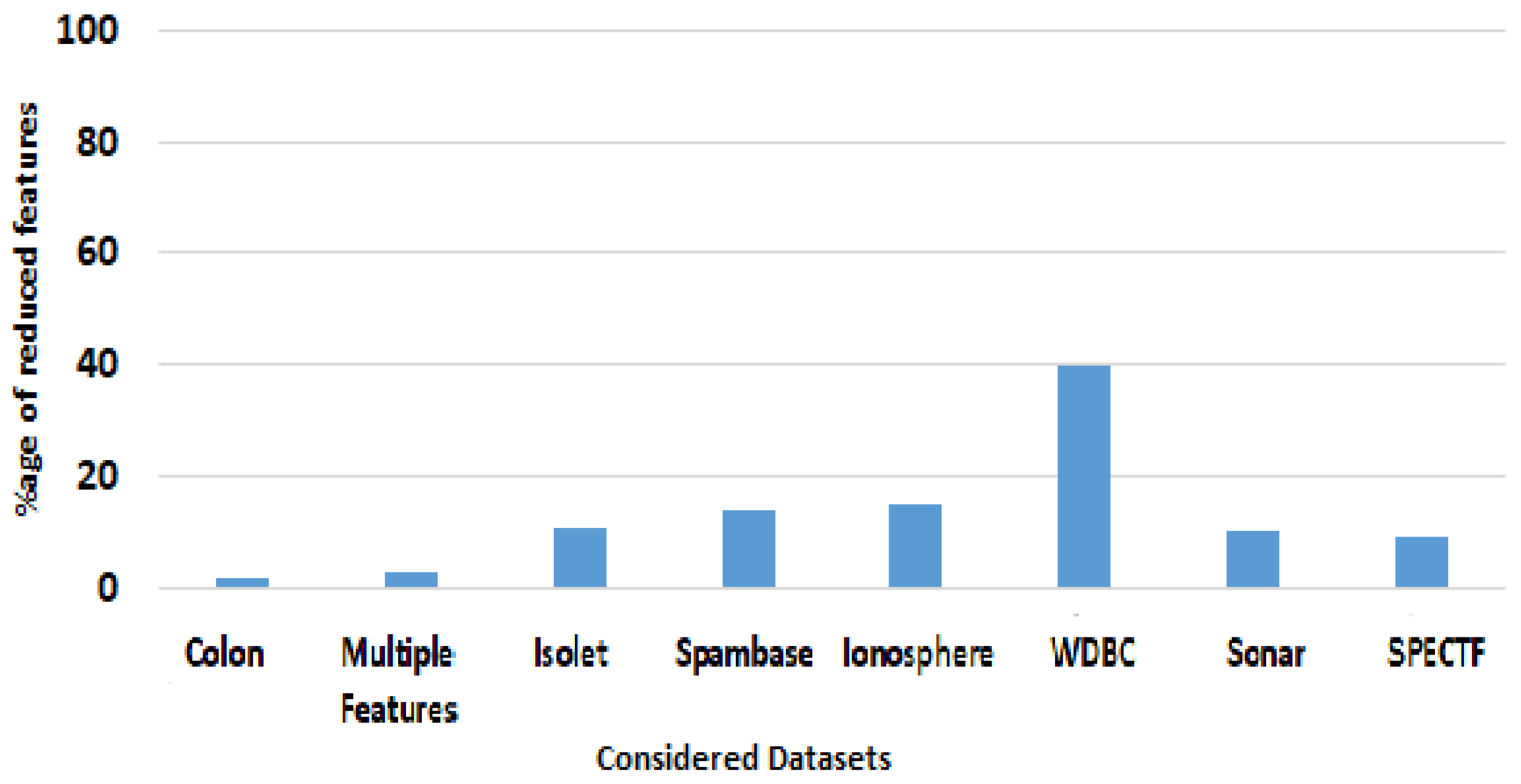
4.1. Considered Dataset

The performance of the proposed method is evaluated on eight publicly available UCI datasets [28] namely, Colon, Multiple Features, Isolet, Spambase, Ionosphere, WDBC, Sonar (Connectionist Bench), and SPECTF. Table 1 details the considered datasets in terms of the number of features, classes, and sample size of the considered dataset. It can be observed from Table 1 that the range of feature size in considered datasets varies extremely, which will evaluate the consistency of the proposed method.

4.2. Performance Evaluation

Two popular metrics are considered for the performance evaluation of the proposed method namely, classification accuracy (ACC) and Matthews correlation coefficient (MCC). Equations (8) and (9) depict the mathematical formulation of ACC and MCC, respectively.
A C C = T P + T N T P + T N + F P + F N
M C C = ( T P     T N ) ( F P     F N ) ( T P + F P ) ( T P + F N ) ( T N + F P ) ( T N + F N )
where, TP, TN, FP, and FN correspond to True Positive, True Negative, False Positive, and False Negative, respectively.
For each feature selection method, 10-fold cross-validation is performed to calculate mean ACC and mean MCC along with respective standard deviations. Further, the classification performance of the considered feature selection methods is evaluated on four classification models, namely K-Nearest Neighbors (KNN), Naïve-Bayes, Support Vector Machine (SVM), and Adaboost.
In the KNN classifier, K is considered the square root of the data size. For the SVM classifier, RBF kernel is used with the parameters according to grid search. Finally, Naïve Bayes is used as the base estimator in the Adaboost classifier. For other parameters, the default values are referred from the respective literature.

5. Performance Analysis

Table 2 and Table 3 demonstrate the performance of the considered feature selection methods on different classifier models in terms of mean ACC and mean MCC, respectively. From the table, it can be observed that the proposed method, DFG-A-DFC, has achieved the best results for more than 50%. The runner-up is DSFFC in terms of overall best classification accuracy. Further, Figure 2 illustrates the visual comparison of the feature-selection methods in the form of a bar chart. In the figure, the x-axis corresponds to the considered methods, while the y-axis depicts the number of times the best value is reported by a method on both parameters, i.e., ACC and MCC. It is clearly envisaged that DFG-A-DFC is best as it reports the best value for the maximum number of times among the considered methods.
Further, Figure 3a depicts the comparison of the considered feature-selection methods with different classifiers on the number of datasets on which each has reported the best value for the ACC parameter. From the figure, it is visible that the proposed method, DFG-A-DFC, with SVM classifier has outperformed other methods on 87% of the considered datasets. Similarly, DFG-A-DFC with KNN and Naïve Baye was superior on 50% of the datasets. Moreover, the proposed method shows competitive performance with the Adaboost classifier. Further, the same comparison was conducted for the MCC parameter in Figure 3b. Here, DFG-A-DFC with SVM classifier has attained the best value on 5 out of 6 datasets, while it is better on 50% of the datasets with KNN and Naïve Baye. However, FCFS fails to report a best value on any dataset for both parameters.
Further, the proposed feature selection method is analyzed in the terms of the reduction in the selected features. Figure 4 illustrates a bar chart for the percentage of the reduced features by considered method on the considered datasets. It can be observed that the proposed method, DFG-A-DFC, has attained a maximum reduction of 40% on the WDBC dataset. While the DFG-A-DFC method is competitive on other datasets. Therefore, it can be claimed that the proposed method is an efficient feature selection method.
Moreover, this paper presents an ablation study on the two-phase architecture of the proposed method. It focuses on studying the performance of the proposed method after the second phase. Table 4 highlights the classification accuracy (ACC) of the proposed method after the first and second phases with different classifiers for each considered dataset. It is notable that the proposed method has shown significant improvement in classification accuracy for each dataset after the second phase. Therefore, it can be concluded that the inclusion of the second phase has strengthened the proposed method.

6. Conclusions

In this paper, a new unsupervised feature selection method, densest feature graph augmentation with disjoint feature clusters (DFG-A-DFC), has been proposed. The proposed method represents the feature set as a graph with the dissimilarity between features as the edge weights. In the first phase, the features selected in the densest subgraph are considered the initial feature subset. In the second phase, shared nearest-neighbor-based clustering is applied to the feature set. Lastly, the final feature subset is formed from the augmentation of the initial feature subset with representative features from the formed clusters. To validate the efficiency of the proposed method, eight UCI datasets have been considered and compared against four existing unsupervised feature selection methods in terms of two performance criteria, namely classification accuracy and Mathews correlation coefficient. Experiments demonstrate that the proposed method is an efficient method in reducing the number of features along with better performance. Thus, it can be used as an alternative for performing feature selection. In the future, the proposed method can be applied to real-time applications such as image segmentation, wireless sensor, and data mining. Furthermore, the proposed method can be extended to big data.

Author Contributions

Conceptualization, D.C. and A.S.; Data curation, D.C., R.C. and H.M.; Formal analysis, D.C., H.M., R.C. and E.Y.; Funding acquisition, A.S. and M.P.; Methodology, D.C., A.S., H.M. and R.C.; Project administration, E.Y. and M.P.; Resources, A.S. and M.P.; Software, D.C., H.M. and R.C.; Supervision, A.S. and M.P.; Validation, H.M. and M.P.; Visualization, D.C., R.C. and E.Y.; Writing—original draft, D.C. and H.M.; Writing—review and editing, D.C., H.M., A.S., R.C., E.Y. and M.P. All authors have read and agreed to the published version of the manuscript.

Funding

This research received no external funding.

Data Availability Statement

Data is publicly available and can be found here, http://archive.ics.uci.edu/ml (accessed on 22 October 2022).

Conflicts of Interest

The authors declare no conflict of interest.

References

  1. Bolón-Canedo, V.; Sánchez-Maroño, N.; Alonso-Betanzos, A. Recent advances and emerging challenges of feature selection in the context of big data. Knowl.-Based Syst. 2015, 86, 33–45. [Google Scholar] [CrossRef]
  2. Bellman, R. Dynamic Programming; Princeton University Press: Princeton, NJ, USA, 1957; p. 18. [Google Scholar]
  3. Keogh, E.; Mueen, A. Curse of Dimensionality. In Encyclopedia of Machine Learning and Data Mining; Springer: Boston, MA, USA, 2017; pp. 314–315. [Google Scholar] [CrossRef]
  4. Kohavi, R.; John, G.H. Wrappers for feature subset selection. Artif. Intell. 1997, 97, 273–324. [Google Scholar] [CrossRef] [Green Version]
  5. Guyon, I.; Elisseeff, A. An Introduction of Variable and Feature Selection. J. Mach. Learn. Res. Spec. Issue Var. Feature Sel. 2003, 3, 1157–1182. [Google Scholar] [CrossRef]
  6. Bolón-Canedo, V.; Sánchez-Maroño, N.; Alonso-Betanzos, A.; Benítez, J.; Herrera, F. A review of microarray datasets and applied feature selection methods. Inf. Sci. 2014, 282, 111–135. [Google Scholar] [CrossRef]
  7. Forman, G. An extensive empirical study of feature selection metrics for text classification. J. Mach. Learn. Res. 2003, 3, 1289–1305. [Google Scholar]
  8. Setia, L.; Burkhardt, H. Feature Selection for Automatic Image Annotation. Lect. Notes Comput. Sci. 2006, 2, 294–303. [Google Scholar] [CrossRef] [Green Version]
  9. Lin, C.-T.; Prasad, M.; Saxena, A. An Improved Polynomial Neural Network Classifier Using Real-Coded Genetic Algorithm. IEEE Trans. Syst. Man Cybern. Syst. 2015, 45, 1389–1401. [Google Scholar] [CrossRef]
  10. Pal, N.; Eluri, V.; Mandal, G. Fuzzy logic approaches to structure preserving dimensionality reduction. IEEE Trans. Fuzzy Syst. 2002, 10, 277–286. [Google Scholar] [CrossRef]
  11. Zhang, G. Neural networks for classification: A survey. IEEE Trans. Syst. Man Cybern. Part C Appl. Rev. 2000, 30, 451–462. [Google Scholar] [CrossRef] [Green Version]
  12. Bandyopadhyay, S.; Bhadra, T.; Mitra, P.; Maulik, U. Integration of dense subgraph finding with feature clustering for unsupervised feature selection. Pattern Recognit. Lett. 2014, 40, 104–112. [Google Scholar] [CrossRef]
  13. Peng, H.; Long, F.; Ding, C. Feature selection based on mutual information criteria of max-dependency, max-relevance, and min-redundancy. IEEE Trans. Pattern Anal. Mach. Intell. 2005, 27, 1226–1238. [Google Scholar] [CrossRef] [PubMed]
  14. Mittal, H.; Saraswat, M.; Bansal, J.; Nagar, A. Fake-Face Image Classification using Improved Quantum-Inspired Evolutionary-based Feature Selection Method. In Proceedings of the IEEE Symposium Series on Computational Intelligence, Canberra, Australia, 1–4 December 2020; pp. 989–995. [Google Scholar]
  15. Guyon, I.; Gunn, S.; Nikravesh, M.; Zadeh, L. Feature Extraction: Foundations and Applications; Springer: Berlin/Heidelberg, Germany, 2006. [Google Scholar]
  16. Bennasar, M.; Hicks, Y.; Setchi, R. Feature selection using Joint Mutual Information Maximisation. Expert Syst. Appl. 2015, 42, 8520–8532. [Google Scholar] [CrossRef] [Green Version]
  17. Mandal, M.; Mukhopadhyay, A. Unsupervised Non-redundant Feature Selection: A Graph-Theoretic Approach. In Advances in Intelligent Systems and Computing; Springer: Berlin, Heidelberg, 2013; pp. 373–380. [Google Scholar] [CrossRef]
  18. Lim, H.; Kim, D.-W. Pairwise dependence-based unsupervised feature selection. Pattern Recognit. 2020, 111, 107663. [Google Scholar] [CrossRef]
  19. Cai, D.; Zhang, C.; He, X. Unsupervised feature selection for multi-cluster data. In Proceedings of the 16th ACM SIGKDD international conference on Knowledge discovery and data mining-KDD ‘10, Washington, DC, USA, 24–28 July 2010. [Google Scholar] [CrossRef] [Green Version]
  20. Liu, Y.; Liu, K.; Zhang, C.; Wang, J.; Wang, X. Unsupervised feature selection via Diversity-induced Self-representation. Neurocomputing 2016, 219, 350–363. [Google Scholar] [CrossRef]
  21. Zhu, P.; Zuo, W.; Zhang, L.; Hu, Q.; Shiu, S.C. Unsupervised feature selection by regularized self-representation. Pattern Recognit. 2015, 48, 438–446. [Google Scholar] [CrossRef]
  22. Mittal, H.; Saraswat, M. A New Fuzzy Cluster Validity Index for Hyperellipsoid or Hyperspherical Shape Close Clusters with Distant Centroids. IEEE Trans. Fuzzy Syst. 2020, 29, 3249–3258. [Google Scholar] [CrossRef]
  23. Lee, J.; Seo, W.; Kim, D. Efficient information-theoretic unsupervised feature selection. Electron. Lett. 2018, 54, 76–77. [Google Scholar] [CrossRef]
  24. Han, D.; Kim, J. Unsupervised Simultaneous Orthogonal basis Clustering Feature Selection. In Proceedings of the 2015 IEEE Conference on Computer Vision and Pattern Recognition (CVPR), Boston, MA, USA, 7–12 June 2015. [Google Scholar] [CrossRef]
  25. Das, A.; Kumar, S.; Jain, S.; Goswami, S.; Chakrabarti, A.; Chakraborty, B. An information-theoretic graph-based approach for feature selection. Sādhanā 2019, 45, 1. [Google Scholar] [CrossRef]
  26. He, X.; Cai, D.; Niyogi, P. Laplacian Score for Feature Selection. In Proceedings of the 18th International Conference on Neural Information Processing Systems 2005, Vancouver, BA, Canada, 5–8 December 2005; pp. 507–514. [Google Scholar]
  27. Mitra, P.; Murthy, C.; Pal, S. Unsupervised feature selection using feature similarity. IEEE Trans. Pattern Anal. Mach. Intell. 2002, 24, 301–312. [Google Scholar] [CrossRef]
  28. Dua, D.; Graff, C. UCI Machine Learning Repository; University of California, School of Information and Computer Science: Irvine, CA, USA, 2019; Available online: http://archive.ics.uci.edu/ml (accessed on 1 June 2022).
  29. Gakii, C.; Mireji, P.O.; Rimiru, R. Graph Based Feature Selection for Reduction of Dimensionality in Next-Generation RNA Sequencing Datasets. Algorithms 2022, 15, 21. [Google Scholar] [CrossRef]
  30. Das, A.K.; Goswami, S.; Chakrabarti, A.; Chakraborty, B. A new hybrid feature selection approach using feature association map for supervised and unsupervised classification. Expert Syst. Appl. 2017, 88, 81–94. [Google Scholar] [CrossRef]
  31. Yan, X.; Nazmi, S.; Erol, B.A.; Homaifar, A.; Gebru, B.; Tunstel, E. An efficient unsupervised feature selection procedure through feature clustering. Pattern Recognit. Lett. 2020, 131, 277–284. [Google Scholar] [CrossRef]
  32. Bhadra, T.; Bandyopadhyay, S. Supervised feature selection using integration of densest subgraph finding with floating forward–backward search. Inf. Sci. 2021, 566, 1–18. [Google Scholar] [CrossRef]
  33. Goswami, S.; Chakrabarti, A.; Chakraborty, B. An efficient feature selection technique for clustering based on a new measure of feature importance. J. Intell. Fuzzy Syst. 2017, 32, 3847–3858. [Google Scholar] [CrossRef]
  34. Kumar, G.; Jain, G.; Panday, M.; Das, A.; Goswami, S. Graph-based supervised feature selection using correlation exponential. In Emerging Technology in Modelling and Graphics; Springer: Singapore, 2020; pp. 29–38. [Google Scholar]
  35. Peralta, D.; Saeys, Y. Robust unsupervised dimensionality reduction based on feature clustering for single-cell imaging data. Appl. Soft Comput. 2020, 93, 10–42. [Google Scholar] [CrossRef]
  36. Das, A.; Pati, S.; Ghosh, A. Relevant feature selection and ensemble classifier design using bi-objective genetic algorithm. Knowl. Inf. Syst. 2020, 62, 423–455. [Google Scholar] [CrossRef]
  37. Saxena, A.; Prasad, M.; Gupta, A.; Bharill, N.; Patel, O.P.; Tiwari, A.; Er, M.J.; Ding, W.; Lin, C.T. A review of clustering techniques and developments. Neurocomputing 2017, 267, 664–681. [Google Scholar] [CrossRef]
  38. Saxena, A.; Chugh, D.; Mittal, H.; Sajid, M.; Chauhan, R.; Yafi, E.; Cao, J.; Prasad, M. A Novel Unsupervised Feature Selection Approach Using Genetic Algorithm on Partitioned Data. Adv. Artif. Intell. Mach. Learn. 2022, 2, 500–515. [Google Scholar]
Figure 1. Block diagram of the proposed method.
Algorithms 16 00028 g001
Figure 2. Bar chart for the number of times the best value is reported by considered methods on ACC and MCC.
Algorithms 16 00028 g002
Figure 3. Comparison of considered feature-selection methods with different classifiers on the number of datasets for which best-value is attained on (a) ACC parameter; and (b) MCC parameter.
Algorithms 16 00028 g003
Figure 4. Comparison of the number of selected features by considered method.
Algorithms 16 00028 g004
Table 1. Details of considered datasets.
Dataset NameNo. of FeaturesNo. of ClassesNo. of Samples
Colon6000262
Multiple Features649102000
Isolet617266238
Spambase5724601
Ionosphere33 *2351
WDBC302569
Connectionist Bench602208
SPECTF44280
* In the ionosphere, there are originally 34 features; but as the second column is the same for all rows, we have not considered it during our experiments.
Table 2. Classification accuracy of different models on considered approaches for various datasets.
DatasetAlgorithmSVMNaive BayesKNNAdaboost
ColonFSFS81.45(0.85)73.39(3.16)74.84(1.56)76.29(3.57)
LSFS71.62(2.04)51.29(1.83)73.55(1.56)60.97(4.35)
MCFS79.52(1.09)67.96(3.41)78.06(1.13)77.10(2.72)
DSFFC82.10(1.19)73.87(1.67)77.42(1.32)79.03(3.48)
DFG-A-DFC86.90(1.44)61.42(1.57)81.90(1.57)56.42(1.81)
None80.71(1.92)58.57(2.64)75.71(1.92)50.47(1.65)
Multiple FeaturesFSFS97.91(0.11)95.51(0.16)94.49(0.21)96.54(0.29)
LSFS97.74(0.11)94.32(0.2)93.02(0.2)96.15(0.20)
MCFS 98.13(0.13)95.59(0.13)95.58(0.13)97.06(0.19)
DSFFC98.35(0.13)94.43(0.12)95.61(0.12)96.22(0.17)
DFG-A-DFC98.60(0.07)96.00(0.12)96.24(0.14)95.55(0.13)
None98.45(0.07)95.49(0.16)96.10(0.11)96.10(0.09)
IsoletFSFS88.17(0.23)65.82(0.21)71.42(0.25)65.78(0.19)
LSFS92.95(0.11)75.49(0.27)82.6(0.19)75.53(0.31)
MCFS95.75(0.12)82.09(0.33)87.99(0.13)81.99(0.21)
DSFFC95.26(0.08)83.61(0.22)86.19(0.14)84.82(0.38)
DFG-A-DFC97.06(0.05)79.99(0.13)88.40(0.12)80.33(0.13)
None97.38(0.06)81.45(0.13)88.69(0.10)81.29(0.18)
SpambaseFSFS78.95(0.11)66.68(0.10)80.81(0.18)66.85(0.15)
LSFS83.84(0.16)69.26(0.11)82.68(0.16)69.28(0.22)
MCFS80(0.09)65.27(0.09)82.27(0.14)65.24(0.12)
DSFFC86.69(0.07)75.63(0.12)84.31(0.11)75.71(0.15)
DFG-A-DFC93.65(0.06)80.06(0.13)86.22(0.12)82.67(0.244)
None93.63(0.11)81.65(0.19)85.95(0.15)83.50(0.25)
IonosphereFSFS91.77(0.49)73.73(0.61)75.41(0.64)85.93(1.36)
LSFS91.37(0.43)76.84(0.71)84.67(0.6)88.83(1.18)
MCFS94.22(0.7)87.89(0.73)82.11(0.6)90.46(0.91)
DSFFC94.07(0.29)89.06(0.57)82.54(0.72)90.85(0.81)
DFG-A-DFC95.73(0.36)89.47(0.60)84.02(0.99)90.31(0.38)
None94.02(0.19)88.88(0.50)84.61(0.62)92.03(0.45)
WDBCFSFS94.41(0.18)91.11(0.22)93.22(0.43)94.22(0.63)
LSFS96.87(0.2)93.71(0.16)95.87(0.21)95.85(0.50)
MCFS96.68(0.24)93.39(0.24)96.22(0.24)95.11(0.44)
DSFFC96.82(0.15)94.34(0.16)95.73(0.17)96.22(0.31)
DFG-A-DFC97.77(0.01)91.73(0.43)95.95(0.02)95.78(0.27)
None97.36(0.21)93.14(0.56)96.13(0.21)97.01(0.22)
SonarFSFS80.24(1.35)70.82(2.41)68.51(1.62)77.16(1.97)
LSFS81.01(1.27)71.88(1.98)67.98(1.20)75.67(1.64)
MCFS82.45(1.04)67.36(1.37)70.14(1.12)77.21(2.07)
DSFFC82.21(1.38)69.42(0.94)71.83(1.09)79.09(1.94)
DFG-A-DFC83.59(1.00)71.21(0.84)72.04(0.99)81.85(0.91)
None83.52(0.99)67.35(0.97)68.64(1.08)79.30(0.819)
SPECTFFSFS73.38(2.13)73.63(1.61)66(1.94)65.50(2.78)
LSFS74(1.42)72.75(1.42)69.63(2.50)69(3.48)
MCFS71.88(2.14)72.13(1.45)66.38(2.32)72.75(3.16)
DSFFC76.88(1.79)79.75(1.84)68.13(1.59)76.88(1.79)
DFG-A-DFC80.00(1.39)80.00(1.39)67.50(0.16)82.50(0.99)
None78.75(1.25)78.75(1.68)65.00(2.07)77.5(1.22)
Table 3. MCC of different models on the considered approaches for various datasets.
DatasetAlgorithmSVMNaive BayesKNNAdaboost
ColonFSFS0.585(0.02)0.439(0.07)0.439(0.044)0.465(0.092)
LSFS0.336(0.061)0.16(0.042)0.406(0.052)0.232(0.088)
MCFS0.54(0.026)0.347(0.076)0.528(0.025)0.495(0.056)
DSFFC0.600(0.028)0.461(0.039)0.512(0.037)0.537(0.084)
DFG-A-DFC0.639(0.034)0.202(0.036)0.559(0.040)0.242(0.033)
None0.399(0.394)0.257(0.051)0.434(0.038)0.170(0.034)
SpambaseFSFS0.554(0.002)0.456(0.002)0.613(0.004)0.459(0.003)
LSFS0.659(0.004)0.497(0.002)0.633(0.003)0.497(0.004)
MCFS0.586(0.002)0.451(0.002)0.624(0.003)0.449(0.002)
DSFFC0.719(0.002)0.585(0.002)0.668(0.002)0.586(0.002)
DFG-A-DFC0.866(0.012)0.643(0.022)0.709(0.027)0.675(0.036)
None0.865(0.023)0.668(0.035)0.703(0.031)0.688(0.045)
IonosphereFSFS0.823(0.011)0.435(0.013)0.462(0.016)0.689(0.030)
LSFS0.814(0.01)0.521(0.01)0.669(0.013)0.755(0.026)
MCFS0.874(0.015)0.746(0.013)0.615(0.013)0.792(0.020)
DSFFC0.873(0.006)0.766(0.011)0.627(0.017)0.822(0.015)
DFG-A-DFC0.908(0.07)0.770(0.138)0.672(0.160)0.788(0.101)
None0.859(0.058)0.761(0.096)0.673(0.117)0.827(0.094)
WDBCFSFS0.88(0.004)0.809(0.005)0.854(0.01)0.876(0.014)
LSFS0.933(0.004)0.866(0.003)0.912(0.004)0.911(0.011)
MCFS0.929(0.005)0.859(0.005)0.92(0.005)0.895(0.009)
DSFFC0.932(0.003)0.879(0.003)0.909(0.004)0.919(0.007)
DFG-A-DFC0.950(0.02)0.823(0.094)0.915(0.041)0.910(0.059)
None0.944(0.04)0.855(0.114)0.918(0.044)0.938(0.045)
SonarFSFS0.606(0.026)0.415(0.048)0374(0.036)0.541(0.039)
LSFS0.620(0.026)0.438(0.039)0.360(0.027)0.511(0.033)
MCFS0.650(0.021)0.379(0.026)0.408(0.024)0.543(0.042)
DSFFC0.642(0.028)0.409(0.020)0.440(0.022)0.580(0.039)
DFG-A-DFC0.691(0.184)0.438(0.170)0.458(0.146)0.647(0.162)
None0.679(0.200)0.353(0.172)0.390(0.236)0.589(0.166)
SPECTFFSFS0.493(0.039)0.480(0.032)0.424(0.037)0.312(0.055)
LSFS0.513(0.030)0.474(0.029)0.472(0.060)0.381(0.069)
MCFS0.479(0.039)0.468(0.028)0.383(0.047)0.458(0.066)
DSFFC0.540(0.033)0.600(0.038)0.468(0.027)0.540(0.033)
DFG-A-DFC0.529(0.327)0.600(0.283)0.433(0.029)0.666(0.221)
None0.489(0.282)0.591(0.326)0.433(0.029)0.590(0.242)
Table 4. Ablation study of the proposed method in terms of ACC parameter.
DatasetAlgorithmSVMNaive BayesKNNAdaboost
ColonFirst Phase74.04(0.82)57.61(1.65)78.33(2.13)52.14(1.53)
Second Phase86.90(1.44)61.42(1.57)81.90(1.57)56.42(1.81)
Multiple FeaturesFirst Phase97.44(0.05)87.79(0.23)92.15(0.16)83.44(0.26)
Second Phase98.60(0.07)96.00(0.12)96.24(0.14)95.55(0.13)
IsoletFirst Phase33.50(0.21)21.00(0.13)31.66(0.14)18.78(0.19)
Second Phase97.06(0.05)79.99(0.13)88.40(0.12)80.33(0.13)
SpambaseFirst Phase79.24(0.13)55.05(0.24)55.98(0.24)79.04(0.11)
Second Phase93.65(0.06)80.06(0.13)86.22(0.12)82.67(0.244)
IonosphereFirst Phase93.72(0.25)87.15(0.72)82.61(0.53)89.15(0.51)
Second Phase95.73(0.36)89.47(0.60)84.02(0.99)90.31(0.38)
WDBCFirst Phase82.08(0.62)77.32(0.43)80.67(0.37)81.18(0.26)
Second Phase97.77(0.01)91.73(0.43)95.95(0.02)95.78(0.27)
SonarFirst Phase64.45(0.57)65.30(1.00)62.50(0.84)63.50(0.86)
Second Phase83.59(1.00)71.21(0.84)72.04(0.99)81.85(0.91)
SPECTFFirst Phase70.00(1.39)78.75(0.80)64.50(1.39)70.00(1.39)
Second Phase80.00(1.39)80.00(1.39)67.50(0.16)82.50(0.99)
Disclaimer/Publisher’s Note: The statements, opinions and data contained in all publications are solely those of the individual author(s) and contributor(s) and not of MDPI and/or the editor(s). MDPI and/or the editor(s) disclaim responsibility for any injury to people or property resulting from any ideas, methods, instructions or products referred to in the content.

