


Optimizing Automated Trading Systems with Deep Reinforcement Learning

Abstract
:1. Introduction
- A novel technique based on DRL to optimize parameters for technical analysis strategies is developed.
- Different approaches to parameter optimization for trading strategies are proposed with suitable trading purpose. In short-term trading, the DRL approach outperforms Bayesian Optimization with higher Sharpe ratio and shorter execution time. On the contrary, Bayesian Optimization is better for long term trading purposes.
2. Related Work
3. Research Methodology
3.1. Learning Environment
3.2. Artificial Intelligent Agent
3.3. Learning Mechanism
- Learning environment randomly sampling a data set where each data for .
- The input for DRL algorithm is represented as a one-hot encoded state vector, .
- Given the state vector , a candidate action is selected with the -greedy technique.
- The parameter is computed. Then, it is sent to the learning environment to compute the reward and generate the next scenario (or ).
- The sample tuples is stored in replay buffer for later use in training model.
- When the replay buffer has stored enough samples (≥ the minimum replay buffer size, ), the oldest tuple will be replaced. A batch of samples is sampled randomly from a replay buffer for training.
- The Q-network is updated by minimizing the defined loss function which is similar to training supervised learning model.
- Finally, the target networks are updated after a preset number of steps .
- If the end of the episode is reached, the searching step will be stopped and go back to step 1. Else, increase and go back to step 3.
| Algorithm 1 DRL algorithm for parameter optimization |
|
- An unseen data set D from the learning environment is given.
- The state of the environment is defined as the data set D plus the history of evaluated parameter configurations and their corresponding response.
- Given state vector, an action is suggested.
- The parameter is calculated and sent to the environment. If the end of the episode is reached, go to the next step, else compute the next state , and return to step 3.
- Given state vector and optimal action, the Q-value, , could be computed.
- Finally, the Q-value along with corresponding parameter set is stored to evaluate performance.
3.4. The Trading System
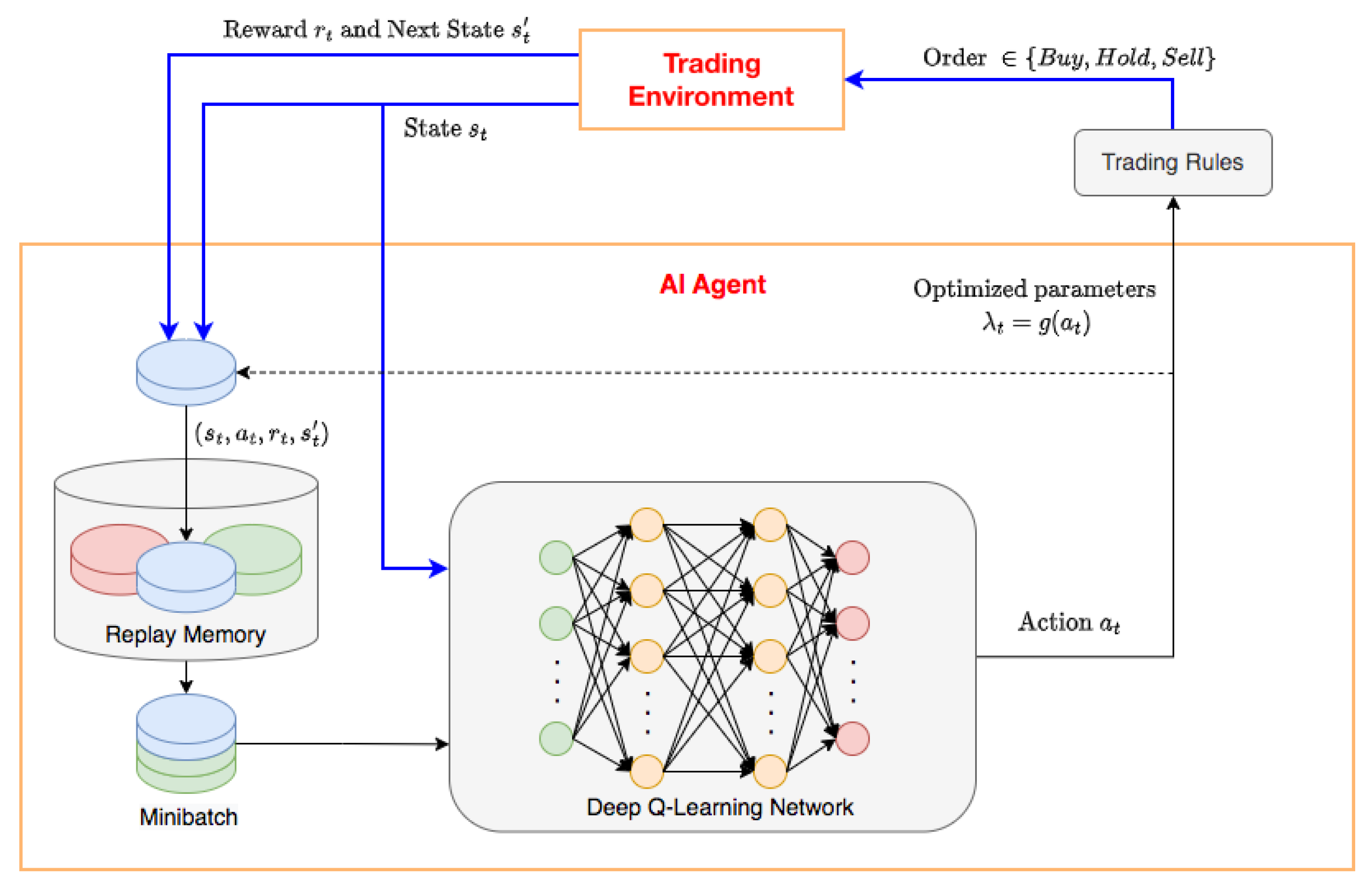
- Learning environment: The trading scenario or state of environment, , is represented as a one-hot encoded vector and decomposed into two parts: the data price , and the sequence of selected parameter configurations and their corresponding rewards, . Given a certain state of the environment, the agent navigates the parameter response surface to select a set of parameters to optimize the reward. He then applies the chosen set of parameters to his trading strategy and executes a sequence of orders (buy, hold or sell) based on the trading rules. These orders are sent to the trading environment to compute the reward and generate the next scenario, .
- Artificial intelligent agent: The aim of the agent is to learn an optimal policy, which defines the probability of selecting a parameter set that maximizes the discounted cumulative return or Sharpe ratio generated from trading strategies.
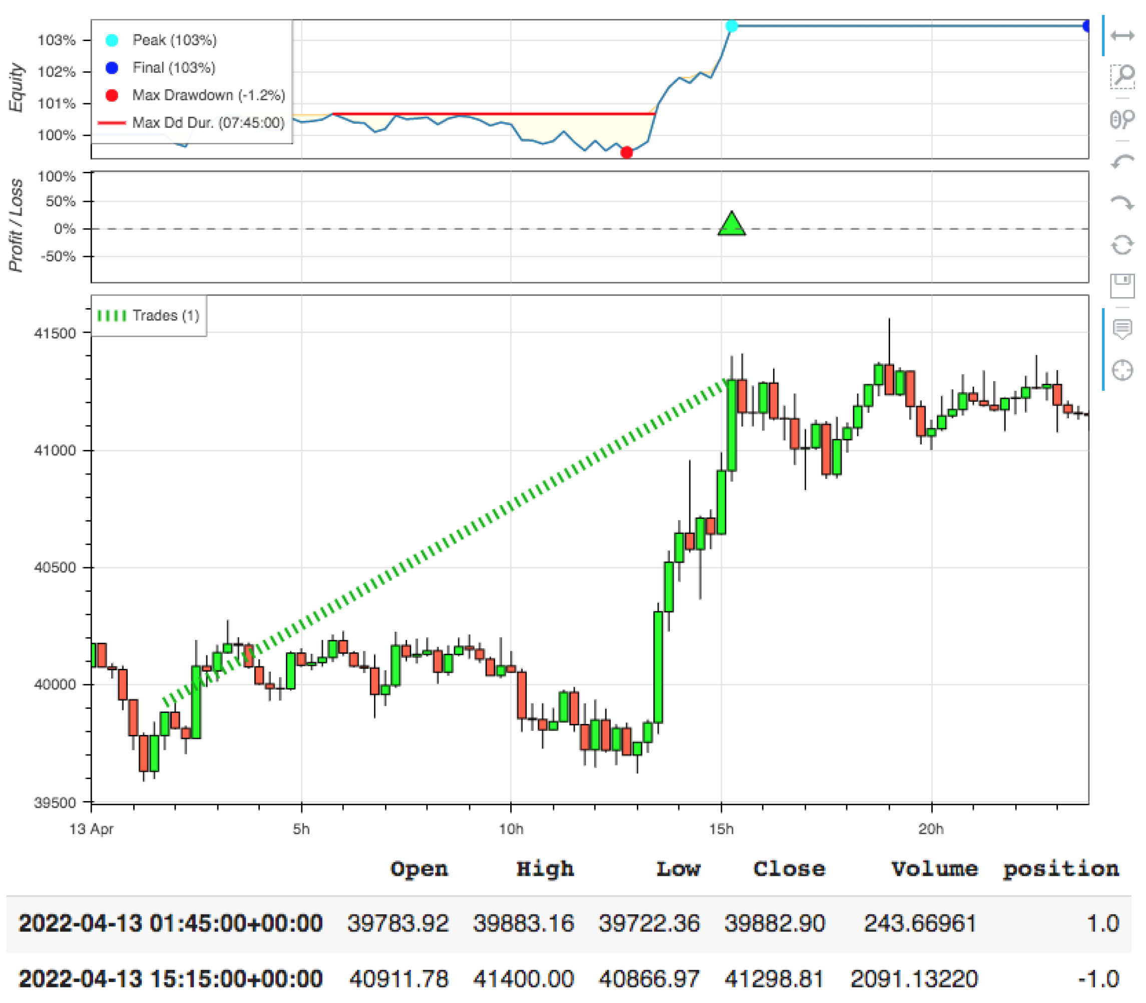
- Learning mechanism: Figure 1 illustrates the interaction between the trader and the trading environment where the arrows show the steps in Algorithm 1. The blue arrows in Figure 1 are the main steps to illustrate a general DRL problem with experience replay. In the proposed environment, the agent can take a random action with probability, , or follow the policy that is believed to be optimal with probability, . An initial value for epsilon of the -greedy action, , is selected for the first observations and then is set to a new value, , after a number of observations. The learning process of agents can be built on a Deep Q-Learning Network. During the trading process, the trader executes orders and calculates the performance through a backtesting step. In our experiment, the trading strategy is built with the common and simple indicator RSI (see [30] for detailed definition). However, the algorithm can be applied to any other technical indicator. The trading rules are presented as follows. A buy signal is produced when RSI falls below oversold zone () and rises above 30 again. When the RSI rises above the overbought zone () and falls below 70 again, a sell signal is obtained.
- Neural network architecture: to approximate the action-value function, architecture of the Deep Neural Network (DNN) can be built using Convolutional Neural Network (CNN) or classical feedforward DNN. In [27], the classical feedforward DNN with leaky rectified linear unit (Leaky ReLU) activation function is used due to the different nature of the input which is time series in our case. CNN is usually used with image input; however, CNN can still be used with an univariate time series, as input as in [31]. CNNs are appropriate for multivariate time series with use of features extracted via the convolutional and the pooling layers. Because of the potential for applying data other than price such as volume, multiple moving average time series, CNN is applied in our network.
- Double DQN and Dueling DQN: These two networks are improved versions of regular DQN. The double DQN uses two networks to avoid over-optimistic Q-values and, as a consequence, helps us train faster and have more stable learning [32]. Instead of using the Bellman equation as in the DQN algorithm, Double DQN changes it by decoupling the action selection from the action evaluation. Dueling DQN separates the estimator using two new streams, value and advantage; they are then combined through a special aggregation layer. This architecture helps us accelerate the training. The value of a state can be calculated without calculating the Q-values for each action at that state. From the above advantages, two networks are applied in our model to compare performance and execution time.
- Optimizer: The classical DQN algorithm usually implements the RMSProp optimizer. ADAM optimizer is the developed version of the RMSprop, it is proven to be able to improve the training stability and convergence speed of the DRL algorithm in [29]. Moreover, this algorithm requires low memory, suitable for large data and parameter problems. Therefore, the ADAM algorithm is chosen to optimize the weights.
- Loss function: Some commonly used functions are Mean Squared Error (MSE) and Mean Absolute Error (MAE). MSE is the simplest and most common loss function; however, the error will be exaggerated if our model gives a very bad prediction. MAE can overcome the MSE disadvantage since it does not put too much weight on outliers; however, it has the disadvantage of not being differentiable at 0. Since outliers can result in parameter estimation biases, invalid inferences and weak volatility forecasts in financial data, to ensure that our trained model does not predict outliers, MSE is chosen as the loss function. In future work, Huber loss can be considered as it is a good trade-off between MSE and MAE, which can make DNN update slower and more stable [27].
4. Experiment
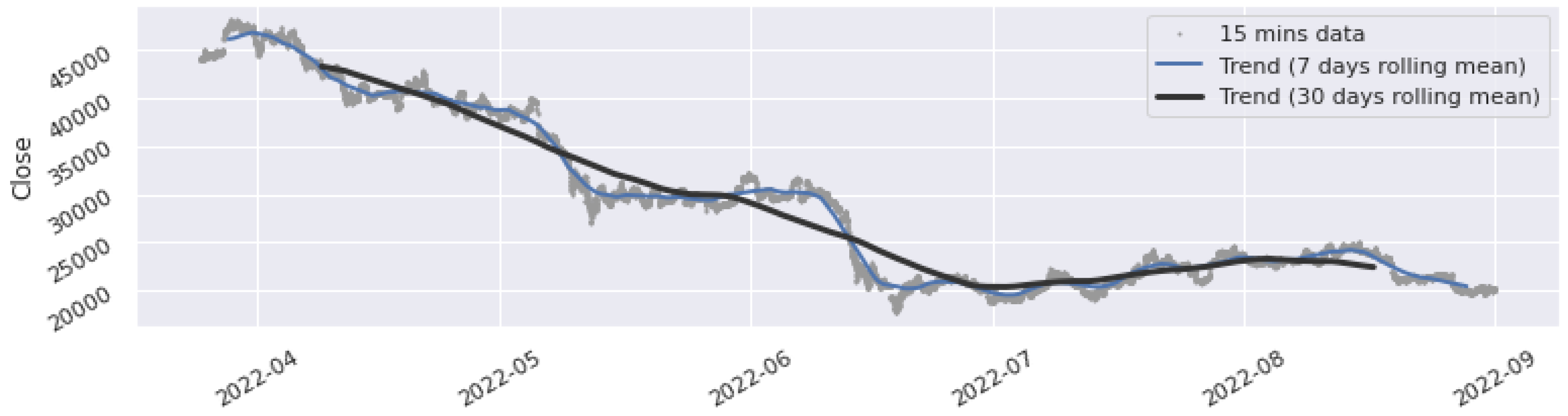
4.1. Dataset
4.2. Experiment Procedure
4.3. Results and Discussion
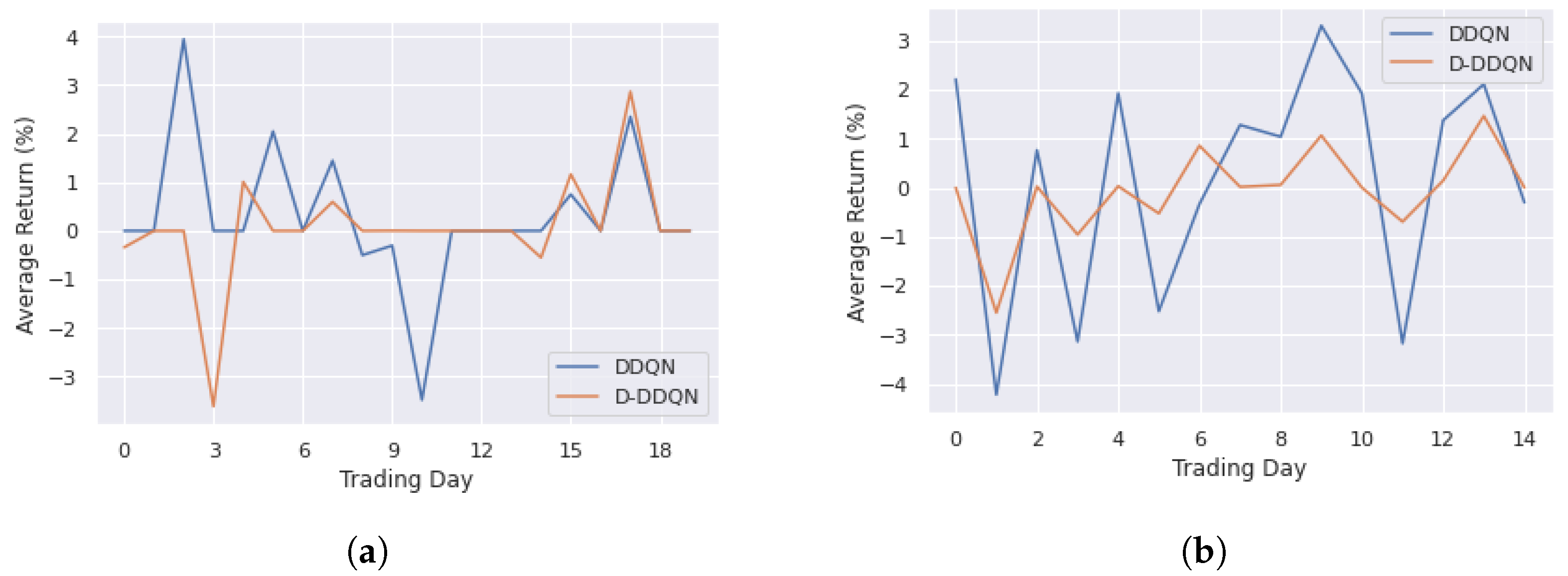
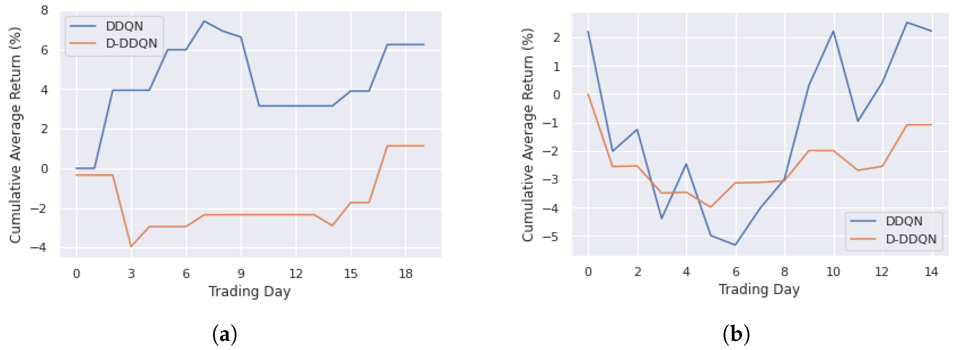
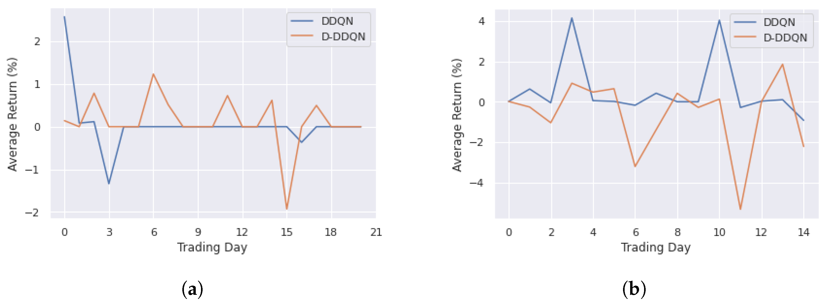
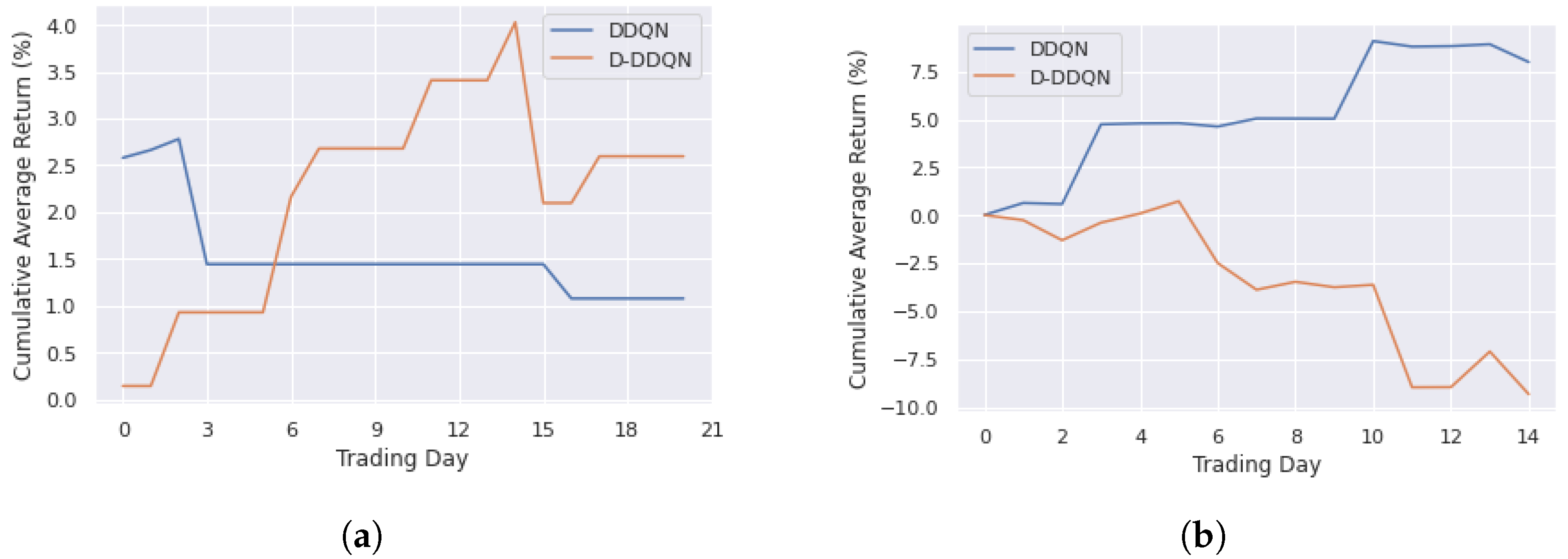
4.3.1. DDQN and D-DDQN Comparision
4.3.2. DRL and Bayesian Optimization Comparision
4.3.3. Execution Time Comparison
5. Conclusions
Author Contributions
Funding
Institutional Review Board Statement
Informed Consent Statement
Data Availability Statement
Conflicts of Interest
Abbreviations
| RL | Reinforcement learning |
| DRL | Deep reinforcement learning |
| BO | Bayesian Optimization |
| RSI | Relative Strength Index |
| SR | Sharpe ratio |
| DDQN | Double Deep Q-Network |
| D-DDQN | Dueling Double Deep Q-Network |
| DNN | Deep Neural Network |
| CNN | Convolutional Neural Network |
References
- Chan, E.P. Quantitative Trading: How to Build Your Own Algorithmic Trading Business; John Wiley & Sons: Hoboken, NJ, USA, 2021. [Google Scholar]
- Xiong, Z.; Liu, X.Y.; Zhong, S.; Yang, H.; Walid, A. Practical deep reinforcement learning approach for stock trading. arXiv 2018, arXiv:1811.07522. [Google Scholar]
- Lucarelli, G.; Borrotti, M. A deep reinforcement learning approach for automated cryptocurrency trading. In Proceedings of the IFIP International Conference on Artificial Intelligence Applications and Innovations, Crete, Greece, 24–26 May 2019; Springer: Berlin/Heidelberg, Germany, 2019; pp. 247–258. [Google Scholar]
- Liu, Y.; Liu, Q.; Zhao, H.; Pan, Z.; Liu, C. Adaptive quantitative trading: An imitative deep reinforcement learning approach. In Proceedings of the AAAI Conference on Artificial Intelligence, New York, NY, USA, 7–12 February 2020; Volume 34, pp. 2128–2135. [Google Scholar]
- Ma, C.; Zhang, J.; Liu, J.; Ji, L.; Gao, F. A parallel multi-module deep reinforcement learning algorithm for stock trading. Neurocomputing 2021, 449, 290–302. [Google Scholar] [CrossRef]
- Pricope, T.V. Deep reinforcement learning in quantitative algorithmic trading: A review. arXiv 2021, arXiv:2106.00123. [Google Scholar]
- Millea, A. Deep reinforcement learning for trading—A critical survey. Data 2021, 6, 119. [Google Scholar] [CrossRef]
- Fayek, M.B.; El-Boghdadi, H.M.; Omran, S.M. Multi-objective optimization of technical stock market indicators using gas. Int. J. Comput. Appl. 2013, 68, 41–48. [Google Scholar]
- Snoek, J.; Larochelle, H.; Adams, R.P. Practical bayesian optimization of machine learning algorithms. Adv. Neural Inf. Process. Syst. 2012, 25, 2951–2959. [Google Scholar]
- Ehrentreich, N. Technical trading in the Santa Fe Institute artificial stock market revisited. J. Econ. Behav. Organ. 2006, 61, 599–616. [Google Scholar] [CrossRef]
- Bigiotti, A.; Navarra, A. Optimizing automated trading systems. In Proceedings of the The 2018 International Conference on Digital Science, Budva, Montenegro, 19–21 October 2018; Springer: Berlin/Heidelberg, Germany, 2018; pp. 254–261. [Google Scholar]
- Snow, D. Machine learning in asset management—Part 1: Portfolio construction—Trading strategies. J. Financ. Data Sci. 2020, 2, 10–23. [Google Scholar] [CrossRef]
- Pardo, R. The Evaluation and Optimization of Trading Strategies; John Wiley & Sons: Hoboken, NJ, USA, 2011; Volume 314. [Google Scholar]
- Wu, J.; Chen, X.Y.; Zhang, H.; Xiong, L.D.; Lei, H.; Deng, S.H. Hyperparameter optimization for machine learning models based on Bayesian optimization. J. Electron. Sci. Technol. 2019, 17, 26–40. [Google Scholar]
- Bergstra, J.; Bengio, Y. Random search for hyper-parameter optimization. J. Mach. Learn. Res. 2012, 13. [Google Scholar]
- Nelder, J.A.; Mead, R. A simplex method for function minimization. Comput. J. 1965, 7, 308–313. [Google Scholar] [CrossRef]
- Kirkpatrick, S.; Gelatt, C.D.; Vecchi, M.P. Optimization by simulated annealing. Science 1983, 220, 671–680. [Google Scholar] [CrossRef]
- Powell, M.J. A direct search optimization method that models the objective and constraint functions by linear interpolation. In Advances in Optimization and Numerical Analysis; Springer: Berlin/Heidelberg, Germany, 1994; pp. 51–67. [Google Scholar]
- Fu, W.; Nair, V.; Menzies, T. Why is differential evolution better than grid search for tuning defect predictors? arXiv 2016, arXiv:1609.02613. [Google Scholar]
- Betrò, B. Bayesian methods in global optimization. J. Glob. Optim. 1991, 1, 1–14. [Google Scholar] [CrossRef]
- Jones, D.R. A taxonomy of global optimization methods based on response surfaces. J. Glob. Optim. 2001, 21, 345–383. [Google Scholar] [CrossRef]
- Ni, J.; Cao, L.; Zhang, C. Evolutionary optimization of trading strategies. In Applications of Data Mining in E-Business and Finance; IOS Press: Amsterdam, The Netherlands, 2008; pp. 11–24. [Google Scholar]
- Zhi-Hua, Z. Applications of data mining in e-business and finance: Introduction. Appl. Data Min. E-Bus. Financ. 2008, 177, 1. [Google Scholar]
- Jomaa, H.S.; Grabocka, J.; Schmidt-Thieme, L. Hyp-rl: Hyperparameter optimization by reinforcement learning. arXiv 2019, arXiv:1906.11527. [Google Scholar]
- Ayala, J.; García-Torres, M.; Noguera, J.L.V.; Gómez-Vela, F.; Divina, F. Technical analysis strategy optimization using a machine learning approach in stock market indices. Knowl.-Based Syst. 2021, 225, 107119. [Google Scholar] [CrossRef]
- Fernández-Blanco, P.; Bodas-Sagi, D.J.; Soltero, F.J.; Hidalgo, J.I. Technical market indicators optimization using evolutionary algorithms. In Proceedings of the 10th Annual Conference Companion on Genetic and Evolutionary Computation, Lille, France, 10–14 July 2008; pp. 1851–1858. [Google Scholar]
- Théate, T.; Ernst, D. An application of deep reinforcement learning to algorithmic trading. Expert Syst. Appl. 2021, 173, 114632. [Google Scholar] [CrossRef]
- Chen, H.H.; Yang, C.B.; Peng, Y.H. The trading on the mutual funds by gene expression programming with Sortino ratio. Appl. Soft Comput. 2014, 15, 219–230. [Google Scholar] [CrossRef]
- Kingma, D.P.; Ba, J. Adam: A method for stochastic optimization. arXiv 2014, arXiv:1412.6980. [Google Scholar]
- Wilder, J.W. New Concepts in Technical Trading Systems; Trend Research: Greensboro, NC, USA, 1978. [Google Scholar]
- Chandra, R.; Goyal, S.; Gupta, R. Evaluation of deep learning models for multi-step ahead time series prediction. IEEE Access 2021, 9, 83105–83123. [Google Scholar] [CrossRef]
- Hessel, M.; Modayil, J.; Van Hasselt, H.; Schaul, T.; Ostrovski, G.; Dabney, W.; Horgan, D.; Piot, B.; Azar, M.; Silver, D. Rainbow: Combining improvements in deep reinforcement learning. In Proceedings of the Thirty-Second AAAI Conference on Artificial Intelligence, New Orleans, LA, USA, 2–7 February 2018. [Google Scholar]
- Gen, M.; Cheng, R. Genetic Algorithms and Engineering Optimization; John Wiley & Sons: Hoboken, NJ, USA, 1999; Volume 7. [Google Scholar]
- Maas, A.L.; Hannun, A.Y.; Ng, A.Y. Rectifier nonlinearities improve neural network acoustic models. In Proceedings of the Icml, Atlanta, GA, USA, 16–21 June 2013; Volume 30, p. 3. [Google Scholar]
- Tieleman, T.; Hinton, G. Neural networks for machine learning. Coursera (Lecture-Rmsprop) 2012, 138, 26–31. [Google Scholar]
- Duchi, J.; Hazan, E.; Singer, Y. Adaptive subgradient methods for online learning and stochastic optimization. J. Mach. Learn. Res. 2011, 12, 2121–2159. [Google Scholar]


| Authors (Year) | Objectives | Findings |
|---|---|---|
| Ni et al. (2008) [22] | Discussing evolutionary technologies to optimize trading strategies Methods: Genetic Algorithms | Genetic Algorithm approach provides better results in terms of returns than typical parameters and Buy&Hold strategy. Genetic Algorithm algorithm can be executed in parallel. |
| Bergstra & Bengio (2012) [15] | Comparing different approaches for neural network optimization Methods: Random Search, Grid Search, Manual Search | Random Search on the same domain in high-dimensional spaces can find better models in less time than Grid Search and Manual Search. |
| Snoek et al. (2012) [9] | Presenting methods to perform BO for hyperparameter selection of general machine learning algorithms Methods: BO with different acquisition functions | BO with Gaussian Process as probabilistic regression model and Expected Improvement as acquisition function signifi- cantly outperforms Tree Parzen Algorithm. BO surpasses a human expert at selecting hyperparameters and beats the state of the art by over 3%. |
| Wu et al. (2019) [14] | Proposing a hyperparameter tuning algorithm for machine learning models Methods: BO, Manual Search | BO algorithm based on Gaussian process can achieve high accuracy and less running time than Manual Search. |
| Jomaa et al. (2019) [24] | Solving hyperparameter optimization problem with RL approach Methods: Random Search, BO, RL | The model based on RL approach does not rely on a heuristic acquisition function like BO. RL method outperforms the Random Search and BO approaches. |
| Ayala et al. (2021) [25] | Optimizing technical analysis strategies using machine learning Methods: Grid Search | Linear model and artificial neural network outperform other machine learning models. The hybrid approach shows improved profits and reduced risk of losses. |
| Parameters | Description | Value |
|---|---|---|
| Number of episodes | 100 | |
| Max capacity of replay memory | 10,000 | |
| Batch size | 40 | |
| Period of Q target network updates | 10 | |
| Discount factor for future rewards | 0.98 | |
| Initial value for epsilon of the -greedy | 1 | |
| Final value for epsilon of the -greedy | 0.12 | |
| Learning rate of ADAM optimizer | 0.001 |
| Period | Setting | Avg. (%) | Max (%) | Min (%) | SD. |
|---|---|---|---|---|---|
| Training | DDQN | 0.31 | 3.95 | −3.48 | 1.39 |
| D-DDQN | 0.06 | 2.87 | −3.61 | 1.10 | |
| Testing | DDQN | 0.15 | 3.30 | −4.22 | 2.26 |
| D-DDQN | −0.07 | 1.46 | −2.55 | 0.90 |
| Period | Setting | Avg. (%) | Max (%) | Min (%) | SD. |
|---|---|---|---|---|---|
| Training | DDQN | 0.05 | 2.58 | −1.34 | 0.64 |
| D-DDQN | 0.12 | 1.24 | −1.93 | 0.58 | |
| Testing | DDQN | 0.53 | 4.15 | −0.93 | 1.44 |
| D-DDQN | −0.62 | 1.8 | −5.34 | 1.76 |
| Avg. Return (%) | Max Return (%) | Min Return (%) | SD. |
|---|---|---|---|
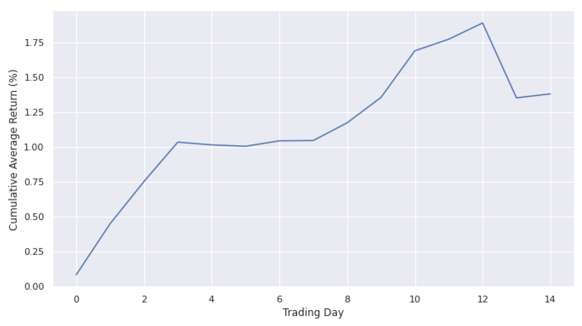
| 1.61 | 28.88 | −22.45 | 9.84 |
| Method | Execution Time (s) |
|---|---|
| DDQN | 6285 |
| D-DDQN | 492 |
| BO | 1435 |
Disclaimer/Publisher’s Note: The statements, opinions and data contained in all publications are solely those of the individual author(s) and contributor(s) and not of MDPI and/or the editor(s). MDPI and/or the editor(s) disclaim responsibility for any injury to people or property resulting from any ideas, methods, instructions or products referred to in the content. |
© 2023 by the authors. Licensee MDPI, Basel, Switzerland. This article is an open access article distributed under the terms and conditions of the Creative Commons Attribution (CC BY) license (https://creativecommons.org/licenses/by/4.0/).
Share and Cite
Tran, M.; Pham-Hi, D.; Bui, M. Optimizing Automated Trading Systems with Deep Reinforcement Learning. Algorithms 2023, 16, 23. https://doi.org/10.3390/a16010023
Tran M, Pham-Hi D, Bui M. Optimizing Automated Trading Systems with Deep Reinforcement Learning. Algorithms. 2023; 16(1):23. https://doi.org/10.3390/a16010023
Chicago/Turabian StyleTran, Minh, Duc Pham-Hi, and Marc Bui. 2023. "Optimizing Automated Trading Systems with Deep Reinforcement Learning" Algorithms 16, no. 1: 23. https://doi.org/10.3390/a16010023
APA StyleTran, M., Pham-Hi, D., & Bui, M. (2023). Optimizing Automated Trading Systems with Deep Reinforcement Learning. Algorithms, 16(1), 23. https://doi.org/10.3390/a16010023