Stochastic Local Community Detection in Networks

Abstract

We propose a stochastic agglomerative algorithm to detect the local community of some given seed vertex/vertices in a network. Instead of giving a deterministic binary local community in the output, our method assigns every vertex a value that is the probability that this particular vertex would be in the local community of the seed. The proposed procedure has several advantages over the existing deterministic algorithms, including avoiding random tie-breaking, evaluating uncertainties, detecting hierarchical community structure, etc. Synthetic and real data examples are included for illustration.

1. Introduction

The structure of complex networks, such as social, metabolic, economic, and informational networks, has been an active research area of network science in the past decades [1,2,3,4]. An interesting area in network science is detecting the community structure in complex networks. Loosely speaking, a community is qualitatively defined as a group of vertices whose interconnected edges are much denser than the edges connecting vertices outside of the group. Communities exist in all types of networks and play an important role in the underlying structure, dynamics, and evolution of the network. Vertices belonging to a tightly bounded group tend to have some common properties. Details on community detection algorithms can be found in [5,6].

While partitioning the whole network requires its global structure information, it is sometimes more desirable to find out the local community starting from a seed, either a single vertex or a group of vertices. For instance, it would be impractical to divide more than two billion Facebook users into separate communities. In another example, the World Wide Web (WWW) is a dynamic network whose global structure is too large to be fully known at any given time point. Instead, a more reasonable question would be to find out those users who are closely related to a given person in his/her social network or to find out all topically related websites starting from a seed page. Bagrow and Bollt proposed an agglomerative L-shell method where vertices are added to the local community based on their geodesic distance from the origin [7]. Papadopoulos et al. introduced a similar method, bridge bounding, which identifies edges that act as boundaries to the local community [8,9]. Clauset proposed a greedy maximization algorithm for finding a local community iteratively through a local modularity measure [10]. While Clauset’s algorithm is intuitive in concept and straightforward to implement [10,11], it does have some drawbacks. At an intermediate iteration, if two vertices lead to the same amount of increase in the local modularity, the tie will be broken randomly. As a result of that, two completely different local communities can be found. Moreover, the output is only qualitative such that any vertex is either included in or excluded from the local community. A numerical measure that quantifies the likelihood of being in the local community would be more informative. Further, a deterministic algorithm may be stuck in local optima, i.e., solutions with the sub-optimal path in which further addition of vertices leads to worse solutions. These drawbacks are common for deterministic algorithms.

In this paper, we propose a stochastic algorithm to search for local communities that can remedy the aforementioned limitations and provide more information on the underlying structure of the network. The paper is organized as follows. In Section 2, a stochastic agglomerative search algorithm is introduced. Its advantages over existing methods are illustrated. In Section 3, the proposed algorithm is applied to synthetic datasets to justify its validity. It is further utilized on the well-known Zachary’s karate club data and Lusseau’s network of bottlenose dolphins. In Section 4, some discussions and conclusions are presented.

2. Materials and Methods

Consider a connected network $\mathcal{G}=(V,E)$ where V and E are the sets of vertices and edges of $\mathcal{G}$, respectively. Suppose $v_0$ is a seed vertex or a group of seed vertices, and we intend to find the local community originating from $v_0$. For example, a web crawler starts from a list of seed web addresses, searches for hyperlinks in the current pages, and visits the newly discovered pages recursively. In a recommendation network, a single item can lead to a group of other topically related items through similar browsing and purchasing history. Several methods have been proposed to identify local communities that lack a global network structure [7,8,10,12]. Among these works, Clauset proposed a very intuitive way of finding the local community in an iterative bottom-up procedure [10]. Let us denote the local community as $\mathcal{C}$. Its neighbor set $\mathcal{U}$ is defined to be those vertices that are not in $\mathcal{C}$ but adjacent to at least one vertex in $\mathcal{C}$. The boundary set $\mathcal{B}$ of $\mathcal{C}$ is defined to be those vertices in $\mathcal{C}$ that have at least one neighbor in $\mathcal{U}$. See Figure 1 for an illustration. A new vertex is added to the current local community one at a time such that the local modularity,

$$R\left(\mathcal{C}\right)=\frac{\mathrm{the}\mathrm{number}\mathrm{of}\mathrm{edges}\mathrm{with}\mathrm{both}\mathrm{ends}\mathrm{in}\mathcal{C}}{\mathrm{the}\mathrm{number}\mathrm{of}\mathrm{edges}\mathrm{with}\mathrm{one}\mathrm{or}\mathrm{more}\mathrm{ends}\mathrm{in}\mathcal{C}},$$

(1)

is increased the most. $R\left(\mathcal{C}\right)$ quantifies the proportion of internal edges of $\mathcal{C}$, and thus can be considered an indicator of the bounding strength in $\mathcal{C}$. Higher value of $R\left(\mathcal{C}\right)$ represents a more tightly bounded group of vertices, which has a higher chance of being a community. It is possible to use other local criteria, e.g., clustering coefficient [13], to define tightly connected local groups.

This algorithm is deterministic in the sense that exactly the same result (local community) will be obtained if we rerun the algorithm starting from the same seed. Moreover, the result is qualitative since a given vertex will be either included in or excluded from the detected local community. In fact, two different vertices in the local community might differ in a quantitative way such that one vertex is closely connected to the seed while the other one barely makes it. Therefore, a more natural and informative way is to gauge the likelihood that a given vertex should be in the local community. Every vertex will be marked by a numerical value such that a higher value implies a larger chance of being in the local community than a lower value.

2.1. A Stochastic Algorithm

We propose an iterative stochastic agglomerative procedure to search for the local community of seed $v_0$. As mentioned before, $v_0$ could be a single vertex or a group of vertices. The local community is still denoted by $\mathcal{C}$, whose element vertices are given by the index set $S_{\mathcal{C}}$. The index sets for $\mathcal{U}$ and $\mathcal{B}$ are represented by $S_{\mathcal{U}}$ and $S_{\mathcal{B}}$, respectively. See Figure 1. At each iteration, a new vertex in $\mathcal{U}$ could be added to $\mathcal{C}$, aiming to increase $R\left(\mathcal{C}\right)$. Meanwhile, a vertex currently already in $\mathcal{C}$ is also subject to removal. Specifically, for each member $v_j$ in $\mathcal{U}$$(j\in S_{\mathcal{U}})$, we compute the change in local modularity $\Delta R_j^A=R(\mathcal{C}+v_j)-R\left(\mathcal{C}\right)$ if $v_j$ is added to $\mathcal{C}$. Meanwhile, we also compute the change $\Delta R_k^R=R(\mathcal{C}-v_k)-R\left(\mathcal{C}\right)$ if a vertex $v_k$ in $\mathcal{C}$ is removed from $\mathcal{C}$ except for those vertices that are either in the seed or whose removal will make $\mathcal{C}$ disconnected. Let $\Delta R=\{\Delta R^A,\Delta R^R\}$ be the changes of all candidate vertices. Instead of choosing the one with the largest increase $\Delta R$, we select a vertex in a probabilistic way.

We introduce a tolerance parameter $ϵ$ that specifies the allowed reduction in $\Delta R$ between iterations. All candidate vertices with $\Delta R<-ϵ$ will not be considered since the reduction in $R\left(\mathcal{C}\right)$ is more than what we can tolerate (points below the dashed line in Figure 2). We randomly select one vertex $v_j$ from the remaining candidates with probability $(\Delta R_j+ϵ)/{\sum }_k(\Delta R_k+ϵ)$. In this way, the vertex with the largest increase will have the largest chance to be selected, but other vertices are not completely eliminated, even though their chances are lower.

Figure 2 shows a toy example of the algorithm on a small network with nine vertices. The seed is vertex 1. The tolerance parameter $ϵ$ is chosen to be 0.05. Three steps are shown where red squares are vertices in the current local community $\mathcal{C}$, and blue circles are the neighbor set $\mathcal{U}$. In the first step (Figure 2a), there are three candidate vertices (3, 4, and 6) to add. The bottom panel of Figure 2a shows the three new $R\left(\mathcal{C}\right)$ values (1/5, 1/5, and 1/6) if each of them is added. The old $R\left(\mathcal{C}\right)$ is 0 (the solid line) since there is only one vertex in $\mathcal{C}$. One of these three vertices is randomly selected based on the increase $\Delta R\left(\mathcal{C}\right)+ϵ$ (the distance from the point to the dotted line). It turns out that vertex 3 is selected, highlighted by the vertical arrow on the plot. Note that any vertex with new $R\left(\mathcal{C}\right)$ below the dotted line will not be considered because it causes a reduction in $R\left(\mathcal{C}\right)$ more than our tolerance level $ϵ$. The dashed line represents the new $R\left(\mathcal{C}\right)$ after the current step with vertices 1 and 3 in $\mathcal{C}$. The second step is shown in Figure 2b, where vertex 9 is added to the local community. Note that we also consider the possibility of removing the existing vertices (vertex 3) from $\mathcal{C}$. In the right panel of Figure 2, vertex 6 is added to $\mathcal{C}$. Removal of vertex 3 is not considered in Figure 2c because it will make the local community disconnected. The algorithm keeps running until no vertices can be added or removed from $\mathcal{C}$; that is, $R\left(\mathcal{C}\right)$ cannot be improved anymore. Subset $\mathcal{C}$, when the algorithm terminates, is one realization of the local community of seed $v_0$. The pseudocode for this process is illustrated in Algorithm 1.

Algorithm 1 The algorithm for the stochastic maximization of local modularity.

add initial seed $v_0$ to $\mathcal{C}$ add all neighbors of $v_0$ to $\mathcal{U}$ set $\mathcal{B}$ to be the boundary of $\mathcal{C}$ compute $R\left(\mathcal{C}\right)$, the local modularity of $\mathcal{C}$ while stopping rules are not satisfied do       choose an adaptive value for $ϵ$       Set $S_{\mathrm{Add}}$ and $S_{\mathrm{Remove}}$ to be empty sets       for each $v_j\in \mathcal{U}$ do             compute $\Delta R_j^A=R_{\mathcal{C}+v_j}-R_{\mathcal{C}}$             insert $\Delta R_j^A$ into $S_{\mathrm{Add}}$       end for       for each $v_k\in \mathcal{C}-v_0$ do             if $\mathcal{C}-v_k$ is connected then                   compute $\Delta R_k=R_{\mathcal{C}-v_k}-R_{\mathcal{C}}$                   insert $\Delta R_k^R$ into $S_{\mathrm{Remove}}$             end if       end for       merge $S_{\mathrm{Add}}$ and $S_{\mathrm{Remove}}$ to get a new set $S_{\mathrm{All}}=S_{\mathrm{Add}}\cup S_{\mathrm{Remove}}$       select one $v_m$ from $S_{\mathrm{All}}$ with probability $\frac{max\{0,\Delta R_m+ϵ\}}{{\sum }_{k}max\{0,\Delta R_k+ϵ\}}$       if $v_m\in \mathcal{U}$ then             add $v_m$ to $\mathcal{C}$       else             remove $v_m$ from $\mathcal{C}$       end if       update $\mathcal{U}$, $\mathcal{B}$, and $R\left(\mathcal{C}\right)$       if stopping rules are satisfied then             break out of the while loop       end if end while

2.2. Tolerance Parameter and Stopping Criteria

Parameter $ϵ$ controls the tightness of the local community. A big value of $ϵ$ allows a big reduction in $R\left(\mathcal{C}\right)$ between iterations. It leads to a larger selection of candidate vertices, thus allowing the algorithm to probe a bigger region of the network at the cost of a longer running time. Using a small value of $ϵ$ allows a small reduction in $R\left(\mathcal{C}\right)$. Therefore, the algorithm will converge faster but might miss some important structures due to the inclusion of fewer candidate vertices. $ϵ=0$ is similar to what was performed in Clauset’s original method, where $R\left(\mathcal{C}\right)$ increases monotonically [10]. In a sense, the algorithm is similar to the simulated annealing optimization using the probabilistic technique to approximate the global optimum of a given function [14]. In practice, a single constant optimal value of $ϵ$ that fits all scenarios does not exist. It depends on the structure of the network, including the clustering, degree distribution, etc. In the initial stage of the algorithm, where there are big fluctuations between consecutive steps, $ϵ$ can be chosen to be large in order to probe a larger area of the network. Later, when $R\left(\mathcal{C}\right)$ stabilizes, $ϵ$ can take smaller values to fine-tune the results.

Certain criteria must be met in order to terminate the algorithm. It is possible that all vertices are included in the local community. More generally, if the local modularity $R\left(\mathcal{C}\right)$ varies little for a certain number of consecutive steps, we then conclude that running the algorithm for more steps will not improve the performance, and it should be terminated.

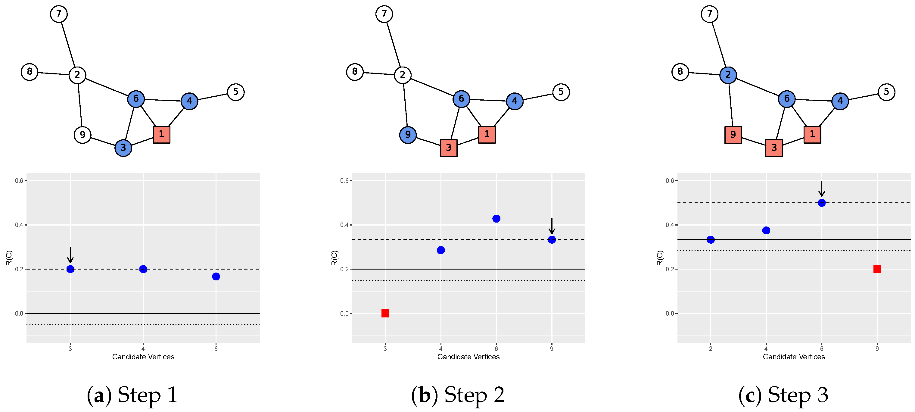
2.3. Evaluation of Inclusion Significance

The procedure outlined in Algorithm 1 needs to be repeated a number of times to receive different realizations of $v_0$’s local community. For each vertex $v_j$ in the network, we compute the proportion of times that it is included in the realizations, denoted by $P_{v_o{v}_j}$, the inclusion probability of $v_j$ in the local community of $v_0$, whose value reveals the community structure around $v_0$. A large value of $P_{v_0{v}_j}$ indicates that vertex $v_j$ has a high likelihood of being in the local community of $v_0$, and vice versa.

A natural question regarding this procedure is that since we potentially could end up with various realizations of the local community, can we simply choose the one with the highest local modularity and use it as the unique “best” result? Actually, this is not the goal of the proposed method. Statistically, the observed network is, in fact, a sample of the actual underlying relationship among network vertices. The output of a deterministic algorithm is a point estimate of the true local community, which is treated as an unknown parameter of the network. It does not convey much information due to the randomness in the sampling procedure. A more informative measure is to assess the significance of the obtained local community, which can be decoded by the inclusion probability.

2.4. Computational Complexity

As discussed in [10], the running time of a single iteration is approximately $O\left(k^{2}d\right)$, where k is the number of vertices in the explored portion of the network or the typical size of the local community, and d is the mean degree of the graph. In the proposed algorithm, we need to run the iteration s times to obtain the inclusion probability. Since the standard error of the inclusion probability is $\sqrt{P(1-P)/s}$ [15], a value of a few hundred for s is sufficient to assure an accuracy of 0.05. In our experiment, s is taken to be 1000.

3. Results

In this section, we will apply the proposed algorithm in both synthetic and real networks for illustration. The data analysis is carried out using the Python package networkx [16].

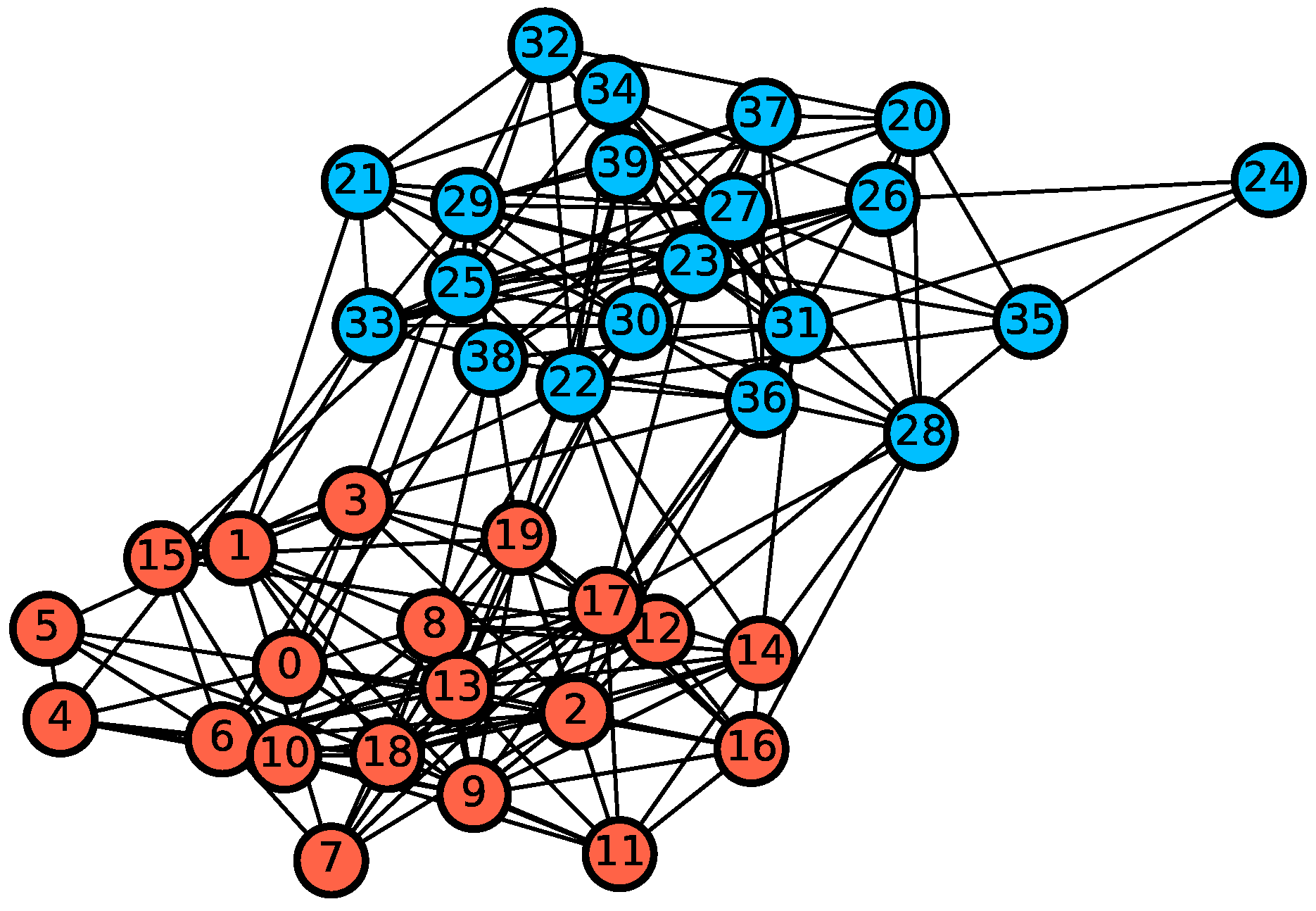
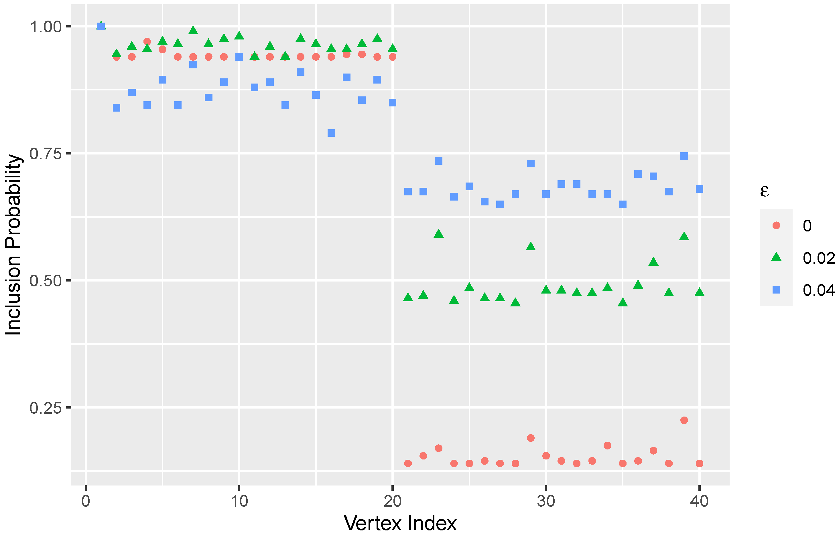
3.1. A Simulation Study

In the simulation study, a synthetic graph is generated from stochastic block model (SBM) with probability matrix $M=\left(\begin{array}{cc}0.5& 0.05\\ 0.05& 0.4\end{array}\right)$ [17]. Each block has 20 vertices. The network is shown in Figure 3.

Since the true community structure is known, we can test the algorithm at different parameters. Figure 4 shows the inclusion probabilities of the local community of vertex 1 by using three constant tolerance parameters, $ϵ=0$, 0.02, and 0.04. It is apparent that the algorithm can detect the underlying hierarchical structure. Meanwhile, as $ϵ$ increases, the inclusion probability also increases for vertices in the other block. This is due to the fact that a broader region in the network is being probed because there is a higher chance of crossing the bridges between the blocks.

As discussed in Section 2.4, the running time scales quadratically with the network size. It is thus feasible to apply the algorithm to a larger network. Moreover, in order to assess the quality of the detected local community, we computed the average inclusion probability ${\overline{P}}_{v_0}$ of all vertices in the same block as the seed $v_0$. A higher value indicates a good quality of the detected community. The same probability matrix M is used on networks with different sizes, and the result is shown in

Table 1. The average inclusion probabilities of vertices in the same block as the seed for different network sizes. N is the number of vertices in the same block as the seed. The total number of vertices in the network is thus $2N$.

N	20	50	100	250	500
${\overline{P}}_{v_0}$	0.913	0.934	0.918	0.925	0.932

. Since all values are higher than 90%, the proposed algorithm performs well on finding the underlying local community structure.

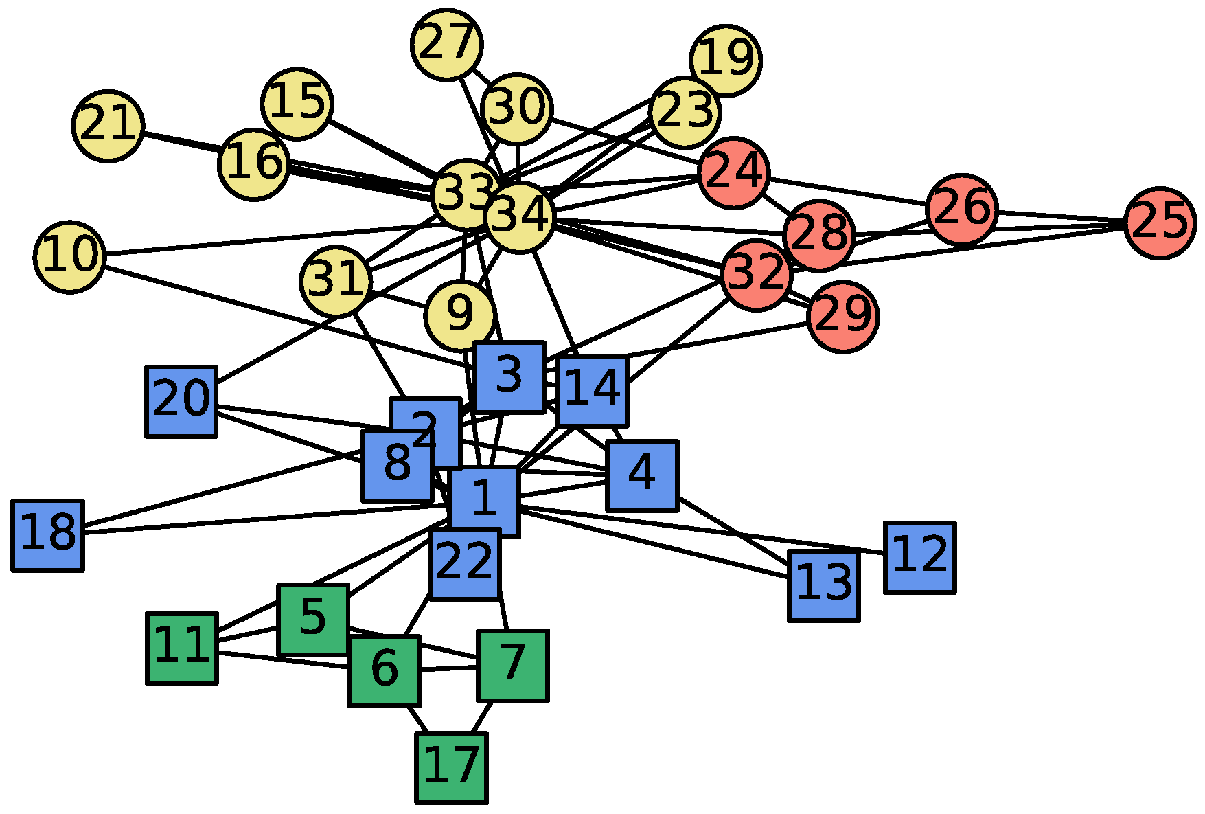
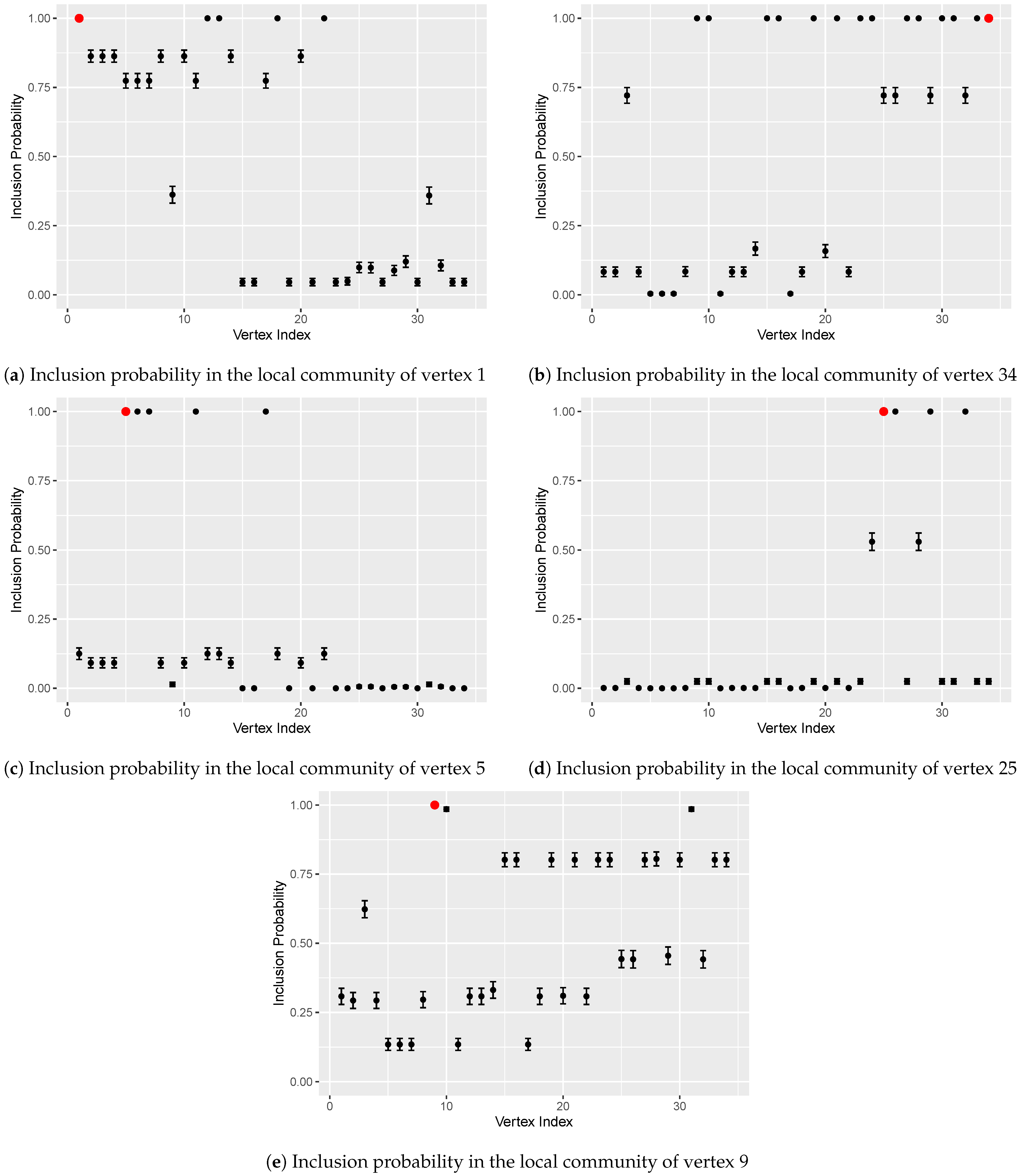
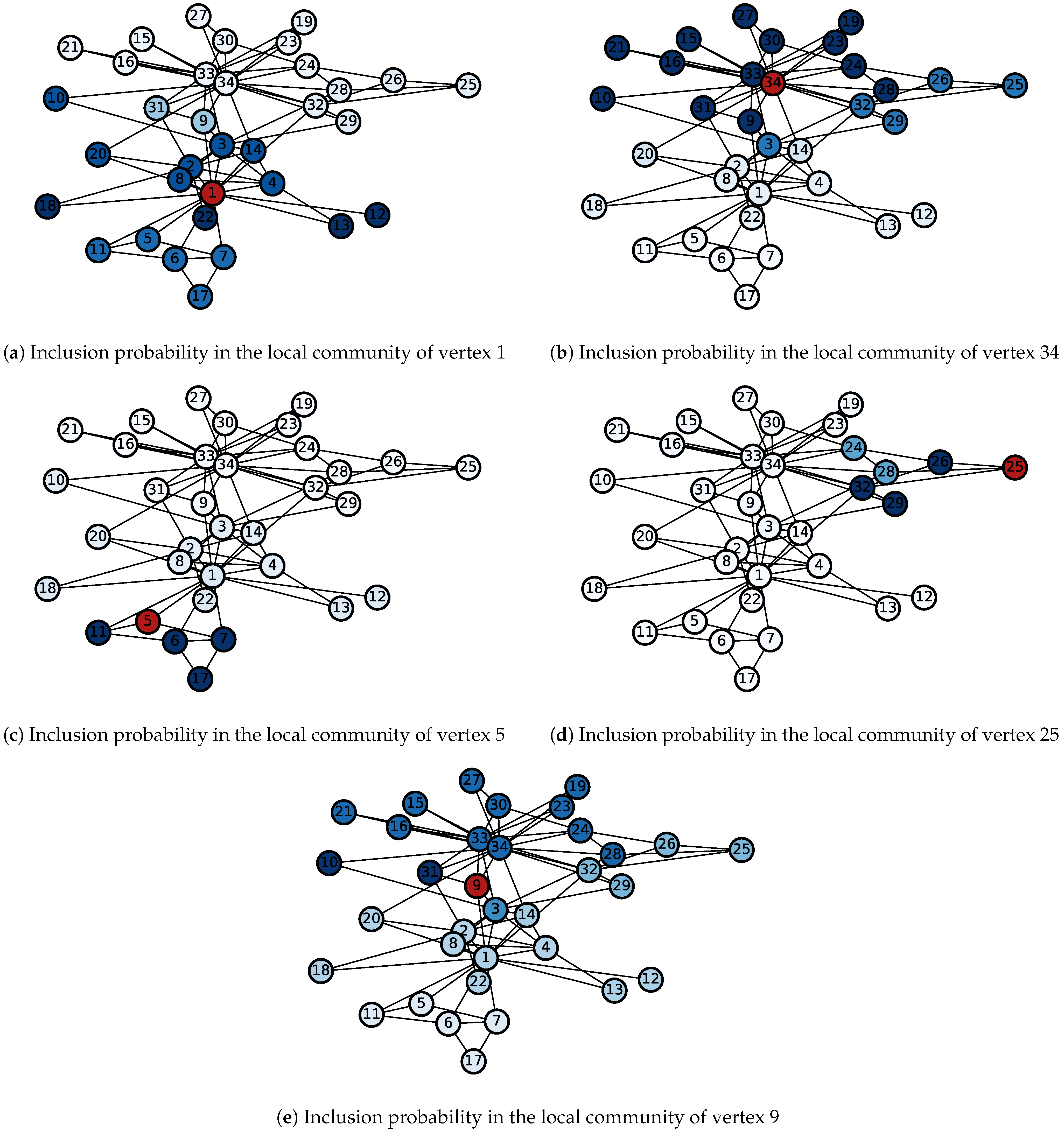
3.2. Zachary’s Karate Club Data

Zachary’s karate club data is a well-known dataset in network science, which contains 34 vertices and 78 edges representing friendship outside the club activities [18]. During the study, a disagreement emerged between the two most central vertices, the instructor (vertex 1) and the administrator (vertex 34), which caused the fission of the club into two smaller groups. Since the actual partition is known, the karate club data set is often used as a benchmark for testing different community detection algorithms. Figure 5 shows the network with the community structure detected by [19]. There are four communities distinguished by different colors and shapes.

We applied the proposed algorithm starting from different seed vertices. For each seed, 1000 realizations are obtained, and the resulting inclusion probabilities are shown in Figure 6 and Figure 7. Algorithms starting from the two central vertices (1 and 34) can recover the actual splitting observed by Zachary, as shown in Figure 6a,b. Additionally, some subdivisions discovered by [19] can also be revealed by the algorithm. Figure 6c and Figure 7c show that the local community of vertex 5 is tightly bounded among the five green vertices in Figure 5. The inclusion probabilities from seed vertex 25 illustrate a similar situation as shown in Figure 6d and Figure 7d, except that the five vertices closely bounded to vertex 25 are at different levels. Vertices 26, 29, and 32 have inclusion probabilities close to 1, which is almost double that of vertex 24 or 28. It is clear that the proposed algorithm can provide a quantitative assessment of the likelihood of being in the local community. A deterministic algorithm cannot do that. Vertices 3, 9, and 10 lie between the two main structures and are easily misclassified by the existing community detection algorithms. Figure 6e and Figure 7e show that the inclusion probabilities from vertex 9 are somewhat homogeneous but lean toward the portion centered around the administrator (vertex 34).

Figure 6e and Figure 7e show an interesting observation. The inclusion probability of vertex 10 is high (∼1) in the local community of vertex 9. However, these two vertices are not even connected. A connection between them would be highly recommended in link predictions [20].

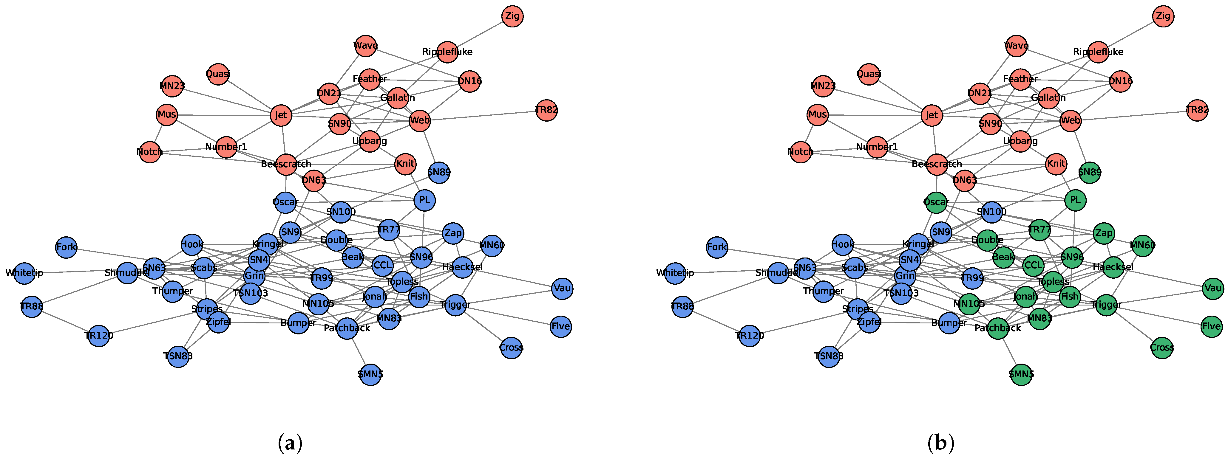
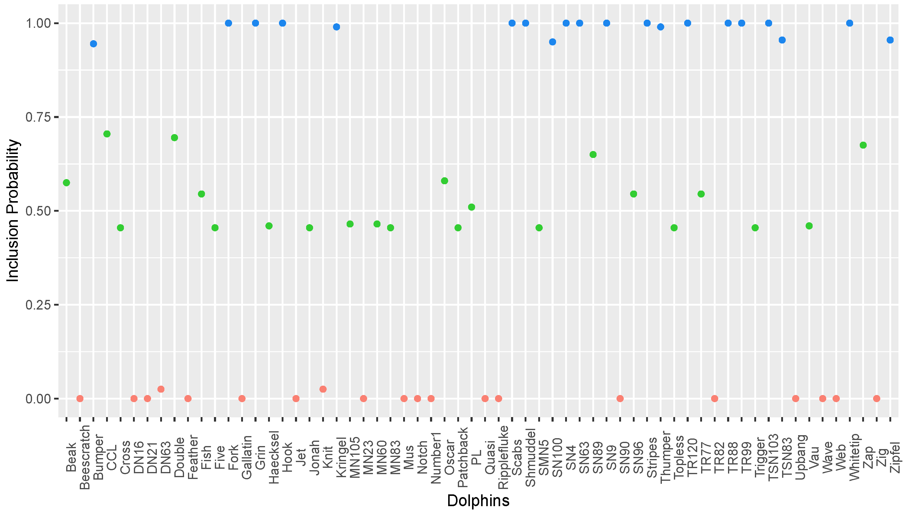
3.3. Lusseau’s Network of Bottlenose Dolphins

The network of social interactions of bottlenose dolphins living in Doubtful Sound, New Zealand, is another popular benchmark data set for community detection [21]. A total of 62 dolphins was observed over a period of 7 years, and edges represent mutual associations occurring more often than by chance. The network was found to have two main communities, as shown in Figure 8a [22]. Using the proposed algorithm and starting from the dolphin named Grin (the one with the highest degree), the inclusion probabilities in its local community are shown in Figure 9. Three different levels are apparent in Figure 8b, with values clustered at (i) close to 1 (blue); (ii) between 0.4 and 0.7 (green); and (iii) close to 0 (red). A cutoff value of 0.4 will lead to exactly the same partition as Figure 8a. The takeaway from the output is that even though both blue and green dots are in the local community of dolphin Grin, there is a difference between the two groups. Blue vertices are tightly connected, while the green vertices are significantly lower in magnitude. The quantification of the communities and discovery of the hierarchical structure are the main advantages of the proposed algorithm.

4. Discussion

In this paper, we propose a stochastic agglomerative algorithm and use a simulated annealing approach to evaluate the local community $\mathcal{C}$ starting from the seed. By iterating the procedure, we obtain the inclusion probabilities of being in the local community for all vertices in the network. The computational complexity has a polynomial scaling with the size of the explored portion of the network and, therefore, is manageable for large networks. The biggest advantage of the proposed method compared to the existing deterministic algorithms is the ability to numerically quantify the output. One can control the tightness of $\mathcal{C}$ by varying the threshold probability. A high threshold will result in a tightly bounded local community in which all vertices are closely related to the seed. Lowering the threshold tends to include more vertices, but some of them may not have a significant connection. This is a tradeoff between diversity and accuracy [23]. Through simulation studies and two real benchmark data sets, the proposed method is shown to be able to reveal the actual underlying community structure by comparing it to existing algorithms. It can shed light on the hierarchical structure of the network, predict new connections in link prediction [20], and provide reliable recommendations in recommender systems [24]. For instance, the inclusion probabilities can be ranked in decreasing order, and then the links between the seed and the top vertices that are not yet connected to the seed should be recommended. Large-scale applications in link predictions and recommender systems are to be addressed in future research.

References

1. Newman, M. Networks: An Introduction; Oxford University Press: Oxford, UK, 2010. [Google Scholar]
2. Newman, M.E. The structure and function of complex networks. SIAM Rev. 2003, 45, 167–256. [Google Scholar] [CrossRef] [Green Version]
3. Strogatz, S.H. Exploring complex networks. Nature 2001, 410, 268. [Google Scholar] [CrossRef] [PubMed] [Green Version]
4. Jackson, M.O. Social and Economic Networks; Princeton University Press: Princeton, NJ, USA, 2010. [Google Scholar]
5. Fortunato, S. Community detection in graphs. Phys. Rep. 2010, 486, 75–174. [Google Scholar] [CrossRef] [Green Version]
6. Fortunato, S.; Hric, D. Community detection in networks: A user guide. Phys. Rep. 2016, 659, 1–44. [Google Scholar] [CrossRef] [Green Version]
7. Bagrow, J.P.; Bollt, E.M. Local method for detecting communities. Phys. Rev. E 2005, 72, 046108. [Google Scholar] [CrossRef] [PubMed] [Green Version]
8. Papadopoulos, S.; Skusa, A.; Vakali, A.; Kompatsiaris, Y.; Wagner, N. Bridge bounding: A local approach for efficient community discovery in complex networks. arXiv 2009, arXiv:0902.0871. [Google Scholar]
9. Rodrigues, F.A.; Travieso, G.; Costa, L.d.F. Fast community identification by hierarchical growth. Int. J. Mod. Phys. C 2007, 18, 937–947. [Google Scholar] [CrossRef] [Green Version]
10. Clauset, A. Finding local community structure in networks. Phys. Rev. E 2005, 72, 026132. [Google Scholar] [CrossRef] [PubMed] [Green Version]
11. Hui, P.; Yoneki, E.; Chan, S.Y.; Crowcroft, J. Distributed community detection in delay tolerant networks. In Proceedings of the 2nd ACM/IEEE International Workshop on Mobility in the Evolving Internet Architecture, Kyoto, Japan, 27–30 August 2007; p. 7. [Google Scholar]
12. Bagrow, J.P. Evaluating local community methods in networks. J. Stat. Mech. Theory Exp. 2008, 2008, P05001. [Google Scholar] [CrossRef] [Green Version]
13. Eckmann, J.P.; Moses, E. Curvature of co-links uncovers hidden thematic layers in the world wide web. Proc. Natl. Acad. Sci. USA 2002, 99, 5825–5829. [Google Scholar] [CrossRef] [PubMed] [Green Version]
14. Kirkpatrick, S.; Gelatt, C.D.; Vecchi, M.P. Optimization by simulated annealing. Science 1983, 220, 671–680. [Google Scholar] [CrossRef] [PubMed]
15. Ott, R.L.; Longnecker, M.T. An Introduction to Statistical Methods and Data Analysis, 7th ed.; Cengage Learning: Boston, MA, USA, 2015. [Google Scholar]
16. Hagberg, A.A.; Schult, D.A.; Swart, P.J. Exploring Network Structure, Dynamics, and Function using NetworkX. In Proceedings of the 7th Python in Science Conference, Pasadena, CA, USA, 19–24 August 2008; pp. 11–15. [Google Scholar]
17. Holland, P.W.; Laskey, K.B.; Leinhardt, S. Stochastic blockmodels: First steps. Soc. Netw. 1983, 5, 109–137. [Google Scholar] [CrossRef]
18. Zachary, W.W. An information flow model for conflict and fission in small groups. J. Anthropol. Res. 1977, 33, 452–473. [Google Scholar] [CrossRef] [Green Version]
19. Donetti, L.; Munoz, M.A. Detecting network communities: A new systematic and efficient algorithm. J. Stat. Mech. Theory Exp. 2004, 2004, P10012. [Google Scholar] [CrossRef] [Green Version]
20. Lü, L.; Zhou, T. Link prediction in complex networks: A survey. Phys. A Stat. Mech. Its Appl. 2011, 390, 1150–1170. [Google Scholar] [CrossRef] [Green Version]
21. Lusseau, D.; Schneider, K.; Boisseau, O.J.; Haase, P.; Slooten, E.; Dawson, S.M. The bottlenose dolphin community of Doubtful Sound features a large proportion of long-lasting associations. Behav. Ecol. Sociobiol. 2003, 54, 396–405. [Google Scholar] [CrossRef]
22. Arenas, A.; Fernandez, A.; Gomez, S. Analysis of the structure of complex networks at different resolution levels. New J. Phys. 2008, 10, 053039. [Google Scholar] [CrossRef] [Green Version]
23. Isufi, E.; Pocchiari, M.; Hanjalic, A. Accuracy-diversity trade-off in recommender systems via graph convolutions. Inf. Process. Manag. 2021, 58, 102459. [Google Scholar] [CrossRef]
24. Vargas, S.; Castells, P. Rank and relevance in novelty and diversity metrics for recommender systems. In Proceedings of the Fifth ACM Conference on Recommender Systems, Chicago, IL, USA, 23–27 October 2011; pp. 109–116. [Google Scholar]
Figure 1. In an intermediate step, the current local community C consists of vertices 1 through 7, in which vertices 1 through 5 (red color) are boundary B . Vertices 6 and 7 (gray color) are the interior of C . The neighbor set U includes vertex 8 through 14 (blue color). The remaining vertices in the network are in white.
Algorithms 16 00022 g001
Figure 2. An illustration of the search algorithm. It shows the first three steps in the search for the local community of vertex 1.
Algorithms 16 00022 g002
Figure 3. A synthetic network generated from the stochastic block model. Red and blue colors represent two underlying blocks, i.e., communities.
Algorithms 16 00022 g003
Figure 4. Plot of inclusion probabilities of vertex 1 in the simulated network in Figure 3. Three tolerance parameters ( ϵ = 0 , 0.02 , and 0.04 ) are used. As ϵ increases, more of the network is probed.
Algorithms 16 00022 g004
Figure 5. Zachary’s karate club data set and its community structure detected by Donetti and Munoz [19]. Each color represents one community. After the splitting of the network, the square vertices are in the subgroup of vertex 1 (instructor), while the round vertices are with vertex 34 (administrator).
Algorithms 16 00022 g005
Figure 6. Inclusion probabilities in the local communities starting from five different seeds, which are represented by red dots. (a): vertex 1 (instructor). (b): vertex 34 (administrator). (c): vertex 5. (d): vertex 25. (e) vertex 9. The error bars depict twice the standard error.
Algorithms 16 00022 g006
Figure 7. Inclusion probabilities in the local communities starting from five different seeds. Darker color indicates a higher inclusion probability. (a): vertex 1 (instructor); (b): vertex 34 (administrator); (c): vertex 8; (d): vertex 25; (e): vertex 9. Seed vertices are in red.
Algorithms 16 00022 g007
Figure 8. Community structure of the dolphin social network. (a) Two communities detected by [22]. (b) Inclusion probabilities of dolphin Grin’s local community. Colors correspond to the values in Figure 9.
Algorithms 16 00022 g008
Figure 9. Inclusion probabilities in the local community of dolphin Grin. Colors represent three clusters of magnitude.
Algorithms 16 00022 g009