Article

Optimizing Automated Trading Systems with Deep Reinforcement Learning

1
John von Neumann Institute, Vietnam National University, Ho Chi Minh City 70000, Vietnam
2
CHArt Laboratory EA 4004, EPHE, PSL Research University, 75014 Paris, France
3
Financial Engineering Department, ECE Paris Graduate School of Engineering, 75015 Paris, France
*
Author to whom correspondence should be addressed.
Algorithms 2023, 16(1), 23; https://doi.org/10.3390/a16010023
Submission received: 24 November 2022 / Revised: 20 December 2022 / Accepted: 27 December 2022 / Published: 1 January 2023

Abstract

:
In this paper, we propose a novel approach to optimize parameters for strategies in automated trading systems. Based on the framework of Reinforcement learning, our work includes the development of a learning environment, state representation, reward function, and learning algorithm for the cryptocurrency market. Considering two simple objective functions, cumulative return and Sharpe ratio, the results showed that Deep Reinforcement Learning approach with Double Deep Q-Network setting and the Bayesian Optimization approach can provide positive average returns. Among the settings being studied, Double Deep Q-Network setting with Sharpe ratio as reward function is the best Q-learning trading system. With a daily trading goal, the system shows outperformed results in terms of cumulative return, volatility and execution time when compared with the Bayesian Optimization approach. This helps traders to make quick and efficient decisions with the latest information from the market. In long-term trading, Bayesian Optimization is a method of parameter optimization that brings higher profits. Deep Reinforcement Learning provides solutions to the high-dimensional problem of Bayesian Optimization in upcoming studies such as optimizing portfolios with multiple assets and diverse trading strategies.

1. Introduction

An automated trading system is a type of information-based decision-making system that allows traders to establish specific rules for both entry and exit of trades and is executed automatically through a computer. Various platforms report about 75% of shares traded on United States stock exchanges come from automatic trading systems [1]. In this context, Reinforcement Learning (RL) is applied to change the way classical trading systems work. RL is a self-training system through taking actions with the aim of maximizing rewards and achieving the best results. Therefore, instead of making decisions based on price forecasting explicitly, in this study our models are trained to execute trading positions directly. Over the past few years, the use of RL has been greatly increased in the study of trading in financial markets [2,3,4]. The authors in [3] applied different Deep Reinforcement Learning (DRL) techniques to build an automated cryptocurrency trading system. As a result, The Double Deep Q-learning trading system based on Sharpe ratio reward function was demonstrated to be the most profitable approach for trading bitcoin. In another research, an agent is trained in [2] to learn an adaptive stock trading strategy and showed that the DRL approach outperforms the Buy and Hold strategy in terms of both Sharpe ratio and cumulative return. Although there are many studies on the application of DRL in financial markets, these studies have only focused on identifying trading signals [5,6,7]. In contrast, there is not much research on parameter optimization approaches for trading strategies. Common methods such as Genetic Algorithm [8] or Bayesian Optimization (BO) [9] still have problems with parameter dimensions or expensive costs. From the above analysis, a new approach on parameter optimization for trading strategies in financial markets with high computational performance becomes an urgent need.
In our paper, the trading task is formatted as a decision-making problem in a large and complex action space, which is applicable for employing reinforcement learning algorithms. Specifically, we propose a learning environment, state representation, reward function and learning algorithm for the purpose of strategy optimization in the cryptocurrency market that has not been studied before. The proposed trading system not only focuses on making decisions based on a given strategy, but also includes a parameter optimization step in the trading process. Two configurations are considered to build the artificial intelligence agent in the system: Double Deep Q-Network and Double Deep Q-Network setting. Bayesian Optimization is another approach introduced for comparison purposes. Different objective functions commonly used in trading optimization are also introduced such as cumulative return and Sharpe ratio. The results demonstated that the DRL approach with the Double Deep Q-Network setting and the BO approach yield positive average returns for short-term trading purposes, where the system with the DRL approach yields better results. In terms of execution time, the DRL approach also shows outstanding advantages with an execution time 5.83 times faster than BO approach. When comparing performance with different settings and objective functions, Double Deep Q-Network setting with Sharpe ratio as reward function is the best Q-learning trading system with 15.96% monthly return. The trading strategies are built on the simple Relative Strength Index (RSI) indicator; however, the results in this study can be applied to any technical or market indicator. In summary, our contribution consists of two main components:
  • A novel technique based on DRL to optimize parameters for technical analysis strategies is developed.
  • Different approaches to parameter optimization for trading strategies are proposed with suitable trading purpose. In short-term trading, the DRL approach outperforms Bayesian Optimization with higher Sharpe ratio and shorter execution time. On the contrary, Bayesian Optimization is better for long term trading purposes.
The rest of the paper is organized as follows. First of all, Section 2 introduces the related work. Section 3 presents the research methodology in which the objective functions and parameter optimization algorithm are studied. Next, an automated trading system and experiments are introduced in Section 4. The results and discussion are also presented. Finally, Section 5 concludes this work and proposes directions for future development.

2. Related Work

Trading strategy optimization has emerged as an interesting research and experimental problem in many fields such as finance [10], data science [11] and machine learning [12]. The optimal trading strategies are the result of finding and optimizing the combination of parameters in the strategy to satisfy the profit or risk conditions. Like model optimization, optimization of trading strategies is a process through which a model learns its parameters [13]. There are mainly two kinds of parameter optimization methods, namely manual search and automatic search methods. Manual Search attempts parameter sets manually and requires researchers to have professional background knowledge and practical experience in the research field [14]. This makes it difficult for researchers who are not familiar with the models or data in a new field. Furthermore, the process of optimizing parameters is not easily repeatable. Trends and relationships in parameters are often misinterpreted or missed as the number of parameters and range of values increases.
Many automatic search algorithms have been proposed, for example Grid Search or Random Search [15], to overcome the drawbacks of manual search. Grid Search prevails as the state of the art despite decades of research into global optimization [16,17,18]. This method lists all combinations of parameters and then performs model testing against this list [9]. Although automatic tuning is possible and the global optimal value of the optimization objective function can be obtained, Grid Search is inefficient both in computational time and in computational power. As the number of parameters increases, the number of models to train increases exponentially [19]. To solve this problem, the Random Search algorithm has been proposed. Random Search only randomly selects a finite number of parameters from the list to conduct a model test [15]. By reducing the search space of unimportant parameters, the overall efficiency is improved and the approximate solution of the optimization function can be found. Random Search is efficient with high dimensional space since it does not run enough cases such as Grid Search. However, some complex models require a global optimal result of the objective function [15]; a new optimization method is needed as an alternative to random search.
In complex models, the objective function of the optimization can be either unknown or a black-box function. A very efficient optimization algorithm that optimizes to solve this problem is Bayesian Optimization [20]. Bayesian Optimization uses the results from the previous iteration to decide the next parameter value candidates. So instead of blindly searching the parameter space such as in Grid Search and Random Search, this method advocates the usage of intelligence to pick the next set of parameters which will improve the model performance. Experimental results show that the Bayesian Optimization algorithm outperforms other global optimization algorithms [9,21]. Although BO provides superior results for parameter optimization compared to Grid Search and Random Search, this method also has its disadvantages. The high-dimensional problem of parameters is costly and contradicts the objective of BO.
Another optimization method used in many studies is evolutionary computing. In [22], the authors presented a general definition of the parameter optimization problem and discussed a Genetic Algorithm based on evolutionary computing to the optimization of trading strategies. Evolutionary computing handles the high-dimensional problem well and produces globally optimal or near-optimal solutions efficiently [23].
In recent years, improvements in machine learning have shown some promising results in solving complex objective functions. In [24], the hyperparameter tuning for machine learning models was formulated as a RL problem, then a novel policy based on Q-learning was proposed for navigating high-dimensional hyperparameter spaces. Ref. [25] proposed a hybrid approach, which combines technical analysis rules with machine learning to generate trading signals, and a grid search is applied on the training data to optimize the strategies. The application of the RL framework requires building a complex environment suitable for each research problem and the financial market is no exception. To the best of our knowledge, there is currently no research to build a trading environment with the RL approach for the purpose of parameter optimization.
A summary of the notable findings described in this section is shown in Table 1. The BO approach provides many outstanding findings; however, the high-dimensional problem of parameters is still a matter of concern. On the other hand, RL is a promising approach to solve this problem. Besides, there are few studies on parameter optimization for technical analysis-based trading strategies. Therefore, this paper focuses on a novel approach to parameter optimization based on reinforcement learning in which computational power will be used to solve the mentioned parameter problem. The paper also aims to build a framework for optimizing trading strategies that can be used in the real market.
In the parameter optimization problem, the objective function and evaluation metrics depend on the developed model and the dataset. In financial models, especially in optimizing trading strategies, the common objective functions are cumulative return, profit and maximum drawdown. In [25], net profit and maximum drawdown are optimized with multiple combinations of parameters for technical trading strategies. The authors in [26] also use net profit as the objective function to optimize the indicators using genetic algorithms. Cumulative return is presented in [2] as an objective function to be maximized when designing a trading strategy. Many metrics are studied to help traders evaluate the performance of their optimized strategies through how robust they are or whether they will survive different market conditions. These metrics are generally divided into two main categories. Traders use performance metrics to get a better understanding of an investment’s return while risk metrics are used to measure how much risk is involved in generating that return. Two most popular performance metrics are Sharpe ratio [27] and Sortino ratio [28]. Sharpe ratio indicates how well an equity investment is performing compared to a risk-free investment, Sortino ratio is a variation of Sharpe ratio that only factors in downside risk. Thus, traders often use the Sharpe ratio to evaluate a low-volatility portfolio while the Sortino ratio is used to evaluate a high-volatility portfolio. Common risk metrics are variance, maximum drawdown and value-at-risk. It is worth noting that objective functions can be used as evaluation metrics and vice versa (see [6,26,27]).

3. Research Methodology

In our problem, the goal is to train the artificial intelligence (AI) agent such that given a trading scenario, it could give an optimized parameter set of the trading strategy and earn a possibly highest reward after a finite number of iterations, as quickly as possible. Instead of using classical optimization approaches, we adapt the Deep Q-Learning (DQN) algorithm [24] for our learning model. This approach is proposed because it does not require prior knowledge of how to efficiently optimize a trading strategy, and the learning algorithm is able to self-evolve when being exposed to unseen scenarios. DRL was selected since it increases the potential of automation for many decision-making problems that were previously intractable because of their high-dimensional state and action spaces. In this section, we briefly describe our learning environment and AI agent, discuss the learning process and some implementation considerations. Accordingly, an automated trading system is introduced to optimize the trading strategies of the experiments performed in this work.

3.1. Learning Environment

The parameter optimization problem is formulated as a Markov Decision Process represented by a tuple ( S , A , R , τ ) , where S is the set of possible states, A is the set of legal actions, a reward function R : S × A R and the transition function τ : S × A × R S that generates a new state in a possibly stochastic or deterministic environment 𝜀 .
The scenario or the state of the environment is defined as the data sets D plus the history of evaluated parameter configurations and their corresponding response:
S = D × ( Λ × R ) .
The agent navigates the parameter response space through a series of actions, which are simply the next parameter configurations to be evaluated, and thus the action space corresponds to the space of all parameter configurations through the function g : A Λ . According to the definition of the action space, the agent executes an action from A = { 1 , , | A | } . For example, action a = 1 , a A , corresponds to parameter set λ = g ( a ) = { λ 1 } d i m ( Λ ) and action a = | A | corresponds to parameter set λ = { λ | A | } d i m ( Λ ) .
The parameter response surface can be any performance metric which is defined by the function f : D × Λ R . The response surface is to estimate the value from an objective function of a strategy M λ M , with parameters λ Λ , over a data set D D :
f ( D , λ ) = ( M λ , D ) .
Considering that the agent’s task is to maximize the reward, the reward function is set as the parameter response function, and depends on the data set D and the action selected, as shown below:
R ( D , a ) = f D , λ = g ( a ) .
The observed reward depends solely on the data set and the parameter configuration selected. Once an action is selected, a new parameter configuration is evaluated.
The transition function then generates a new state, s S , by appending the newly evaluated parameter configuration, λ , and the corresponding reward r R observed to the previous state s S :
s = τ ( s , a , r ) = s , ( λ = g ( a ) , r ) .
The agent reaches the terminal state in case of exceeding the prescribed budget T. At each step t T , agent study the data d D , the state s t = ( d t , ( λ 0 , r 0 ) , , ( λ t , r t ) ) and the next step s t + 1 = ( d t + 1 , ( λ 0 , r 0 ) , , ( λ t , r t ) , ( λ t + 1 , r t + 1 ) ) . This means each state s includes all previously parameter configurations and their corresponding response. The budget could be the running time/target reward is reached or the same parameter set is selected twice in a row. The last condition causes the agent to keep on exploring the parameter space without getting stuck in a specific reward configuration.

3.2. Artificial Intelligent Agent

The agent interacts with the environment 𝜀 with the task of maximizing the expected discounted reward. They execute actions from the action space and receive observations and rewards. At each time step, which ranges over a set of discrete time intervals, the agent selects an action a at state s. The behavior of the agent is governed by a stochastic policy, π : S A , which tells the agent which actions should be selected for each possible state. As a result of each action, the agent receives a scalar reward r, and observes the next state s . The policy is used to compute the true state-action value, Q π ( s , a ) , as:
Q π ( s , a ) = E π t = 0 γ t r t | s 0 = s , a 0 = a ,
where γ [ 0 , 1 ] represents the discount factor balancing between immediate and future rewards. This basically helps to avoid infinity as a reward in case the task has no terminal state.
The aim of the agent is to learn an optimal policy which defines the probability of selecting action that maximizes the discounted cumulative reward, π * ( s ) a r g m a x a Q * ( s , a ) , where Q * ( s , a ) denotes the optimal action value. One of the most popular value-based methods for solving RL problems is Q-learning algorithm [29]. The basic version of the Q-learning algorithm makes use of the Bellman equation for the Q-value function, whose unique solution is the optimal value function Q * ( s , a ) :
Q * ( s , a ) = E π r + γ m a x a Q * ( s , a ) | s 0 = s , a 0 = a .

3.3. Learning Mechanism

The interaction between AI agent and learning environment is the core mechanism for training and testing in the RL framework. Starting at a random location in the parameter space of a random data set, the agent needs to navigate the parameter response surface, including the parameter configuration and corresponding reward of a given model. At each step, the agent explores the environment, selects the next best parameter set with the ϵ -greedy technique, and sends it to the environment. The policy ϵ -greedy(Q) to select action a t is defined, as follows:
a t = U n i f ( Λ ) , if x U n i f ( [ 0 , 1 ] ) < ϵ , a r g m a x a Q * ( s t , a ) , otherwise .
Learning environment will update the current state, evaluate it and send feedback back to agent as a reward. When the agent runs out of a number of episodes, he will be relocated to the response surface of another data set. The transitions are stored in the replay memory where a small batch of experiences is sampled to update the Q-network. By using experience replay, it breaks down the successive correlation among samples and also allows the network to make use of experiences better.
Algorithm 1 can be used to describe the learning process of the agent, including training phase and testing phase. The main purposes of the training phase include generating learning samples, training the Deep Q-network using DRL algorithm. While in the testing phase, given an unseen scenario, the target network is used to predict an optimal parameter set. The step by step algorithm for training is as follows.
  • Learning environment randomly sampling a data set D = { d 0 , , d T } where each data d t U n i f ( D ) for t = 1 , , T .
  • The input for DRL algorithm is represented as a one-hot encoded state vector, s 0 = ( d 0 , ( { λ i n i t } d i m ( Λ ) , 0 ) ) .
  • Given the state vector s t , a candidate action a t is selected with the ϵ -greedy technique.
  • The parameter λ t is computed. Then, it is sent to the learning environment to compute the reward r t and generate the next scenario s t (or s t + 1 ).
  • The sample tuples ( s t , a t , r t , s t + 1 ) is stored in replay buffer for later use in training model.
  • When the replay buffer has stored enough samples (≥ the minimum replay buffer size, N B ), the oldest tuple will be replaced. A batch of samples is sampled randomly from a replay buffer for training.
  • The Q-network is updated by minimizing the defined loss function which is similar to training supervised learning model.
  • Finally, the target networks are updated after a preset number of steps N u .
  • If the end of the episode is reached, the searching step will be stopped and go back to step 1. Else, increase t = t + 1 and go back to step 3.
Algorithm 1 DRL algorithm for parameter optimization
1:
Initialize network Q and target network Q ^
2:
Initialize experience replay memory B
3:
Initialize the Agent to interact with the Environment
4:
for N e iterations do                                                                                   ▹ N e - number of episodes
5:
      Randomly sampling a data set D = { d 0 , , d T } , d U n i f ( D )
6:
      Get state s 0 = ( d 0 , ( { λ i n i t } d i m ( Λ ) , 0 ) )
7:
      for  t { 0 , , T } and while s t is not terminal do
8:
             Determine next action a t from state s t using policy ϵ -greedy(Q)        ▹ Equation (7)
9:
             Receive reward r t = R ( d t , λ = g ( a t ) )                                                 ▹ Equation (3)
10:
             Generate new state s t = τ ( s t , a t , r t )                                                    ▹ Equation (4)
11:
             Store transition ( s t , a t , r t , s t ) in the experience replay memory B
12:
             Replace oldest tuple if | B | > N B                                                 ▹ N B - replay buffer size
13:
             if enough experience in B then
14:
                  Sample a random minibatch of N transitions from B
15:
                  for every transition ( s i , a i , r i , s i ) in minibatch do
                     y i = r i ,                       if s i is terminal ; r i + γ m a x a Q ^ ( s i , a ) , otherwise .
16:
                  end for
17:
                  Update Q by minimizing the loss
                        = 1 / K i = 0 K 1 Q ( s i , a i ) y i 2
18:
                  Copy weights from Q to Q ^ for every N u steps
19:
            end if
20:
      end for
21:
end for
The testing phase is relatively simple since we only need to get the final optimized parameter set for a given scenario. However, in practical use, the experiences generated in this phase can also be stored in a replay buffer for tuning the model via batch training. This setting can help the model tuning to be faster and keep the model up-to-date with new incoming data. The step-by-step algorithm for testing is described as follows.
  • An unseen data set D from the learning environment is given.
  • The state of the environment is defined as the data set D plus the history of evaluated parameter configurations and their corresponding response.
  • Given state vector, an action a t * is suggested.
  • The parameter λ t * is calculated and sent to the environment. If the end of the episode is reached, go to the next step, else compute the next state s i + 1 , i = i + 1 and return to step 3.
  • Given state vector and optimal action, the Q-value, Q * ( s , a * ) , could be computed.
  • Finally, the Q-value along with corresponding parameter set λ * is stored to evaluate performance.

3.4. The Trading System

From the concepts for parameter optimization described, in this section, we proceed to build a trading system that can both give trading signals and optimize strategies automatically. To provide the trading environment, we study the state representation and present it in a form that the agent can understand. We propose a definition of an agent’s parameter selection and a mapping from the act of choosing parameters for trading strategies to investment decisions. Each decision can be scored using the proposed reward function. The main components of the proposed system are described as follows.
  • Learning environment: The trading scenario or state of environment, s t , is represented as a one-hot encoded vector and decomposed into two parts: the data price d t D , and the sequence of selected parameter configurations and their corresponding rewards, ( λ t , r t ) ( Λ × R ) . Given a certain state of the environment, the agent navigates the parameter response surface to select a set of parameters to optimize the reward. He then applies the chosen set of parameters to his trading strategy and executes a sequence of orders (buy, hold or sell) based on the trading rules. These orders are sent to the trading environment to compute the reward and generate the next scenario, s t .
  • Artificial intelligent agent: The aim of the agent is to learn an optimal policy, which defines the probability of selecting a parameter set that maximizes the discounted cumulative return or Sharpe ratio generated from trading strategies.
  • Learning mechanism: Figure 1 illustrates the interaction between the trader and the trading environment where the arrows show the steps in Algorithm 1. The blue arrows in Figure 1 are the main steps to illustrate a general DRL problem with experience replay. In the proposed environment, the agent can take a random action with probability, ϵ , or follow the policy that is believed to be optimal with probability, 1 ϵ . An initial value for epsilon of the ϵ -greedy action, ϵ s t a r t , is selected for the first observations and then is set to a new value, ϵ e n d , after a number of observations. The learning process of agents can be built on a Deep Q-Learning Network. During the trading process, the trader executes orders and calculates the performance through a backtesting step. In our experiment, the trading strategy is built with the common and simple indicator RSI (see [30] for detailed definition). However, the algorithm can be applied to any other technical indicator. The trading rules are presented as follows. A buy signal is produced when RSI falls below oversold zone ( R S I < 30 ) and rises above 30 again. When the RSI rises above the overbought zone ( R S I > 70 ) and falls below 70 again, a sell signal is obtained.
In our novel DRL-based parameter optimization method, the DQN algorithm is modified and improved to adapt to the specific trading decision-making problem. The modifications and improvements are summarized as below.
  • Neural network architecture: to approximate the action-value function, architecture of the Deep Neural Network (DNN) can be built using Convolutional Neural Network (CNN) or classical feedforward DNN. In [27], the classical feedforward DNN with leaky rectified linear unit (Leaky ReLU) activation function is used due to the different nature of the input which is time series in our case. CNN is usually used with image input; however, CNN can still be used with an univariate time series, as input as in [31]. CNNs are appropriate for multivariate time series with use of features extracted via the convolutional and the pooling layers. Because of the potential for applying data other than price such as volume, multiple moving average time series, CNN is applied in our network.
  • Double DQN and Dueling DQN: These two networks are improved versions of regular DQN. The double DQN uses two networks to avoid over-optimistic Q-values and, as a consequence, helps us train faster and have more stable learning [32]. Instead of using the Bellman equation as in the DQN algorithm, Double DQN changes it by decoupling the action selection from the action evaluation. Dueling DQN separates the estimator using two new streams, value and advantage; they are then combined through a special aggregation layer. This architecture helps us accelerate the training. The value of a state can be calculated without calculating the Q-values for each action at that state. From the above advantages, two networks are applied in our model to compare performance and execution time.
  • Optimizer: The classical DQN algorithm usually implements the RMSProp optimizer. ADAM optimizer is the developed version of the RMSprop, it is proven to be able to improve the training stability and convergence speed of the DRL algorithm in [29]. Moreover, this algorithm requires low memory, suitable for large data and parameter problems. Therefore, the ADAM algorithm is chosen to optimize the weights.
  • Loss function: Some commonly used functions are Mean Squared Error (MSE) and Mean Absolute Error (MAE). MSE is the simplest and most common loss function; however, the error will be exaggerated if our model gives a very bad prediction. MAE can overcome the MSE disadvantage since it does not put too much weight on outliers; however, it has the disadvantage of not being differentiable at 0. Since outliers can result in parameter estimation biases, invalid inferences and weak volatility forecasts in financial data, to ensure that our trained model does not predict outliers, MSE is chosen as the loss function. In future work, Huber loss can be considered as it is a good trade-off between MSE and MAE, which can make DNN update slower and more stable [27].

4. Experiment

4.1. Dataset

In this experiment, we consider the 15-min historical data (open, high, low and close price) of BTC-USDT from the 25 March 2022 to the 31 August 2022 (15,360 observations). The data are publicly available at https://www.binance.com/en/landing/data, accessed on 1 November 2022. To get more information from the data, trend analysis is applied with two techniques: the rolling means and the distribution of price increments. First, the trend of our data is visualized using rolling means at 7-days and 30-days scales. As shown in Figure 2, we can observe that the overall trend of 30-days rolling closing price is decreasing over time, which indicates that the market is in a major downtrend in a large time frame. In a bearish market, common strategies such as the Buy and Hold strategy are not profitable. In smaller time frames such as the 7-days rolling closing price, the market shows signs of slight recovery from early July to mid-August.
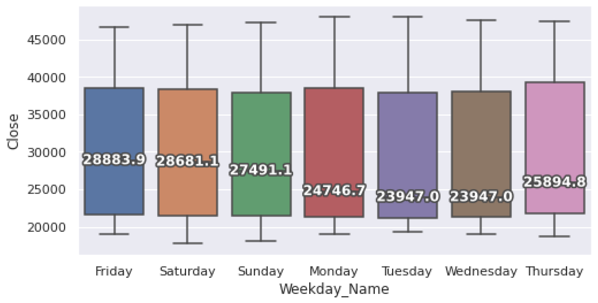
Beside the rolling means, the median values can also be useful for exploratory data analysis. The distribution of price increments for each weekday is plotted in Figure 3. The fluctuation range of all trading days is large, indicating that the seasonal stability is not good. This is consistent with the strong downtrend results of the markets given in the trend analysis step. A good result is that the data does not contain outliers, so we can skip the outlier detection step when pre-processing the data. The median values from Saturday to Tuesday suggest that the crypto market is likely to fall during this time period. Wednesday to Friday is the time when the market goes up again. Saturday’s data is marked by high volatility and the market tends to decrease on this day, so traders can build a strategy to buy on Wednesdays and sell on Saturdays. In addition, intraday trades can also be executed based on strong fluctuations in the minimum and maximum values of the trading days.

4.2. Experiment Procedure

To avoid the case where the optimization techniques are over-fitted or the obtained parameters do not yield any profit in other periods, we consider 100 periods with the size of each period being 3456 observations (36 days). For each period, the start date and end date are different, the first 80% of the dataset is dedicated for training purposes and the remaining 20% is used for testing the performance. This ratio is chosen according to the Pareto principle, which is commonly applied to optimization efforts in computer science [33]. Without a loss of generality, other ratios can also be applied.
The parameters used for training the agent are shown in Table 2. The agent is assumed to start with an initial capital of 1,000,000 and a cost of 0.1% is applied to each executed transaction for a more realistic study. The values of other parameters in the system are selected from practice and from previous studies [3,29,34]. In our case, future rewards play a more important role because of the volatility of the price, so in this study, γ is assigned a value of 0.98. An initial ϵ s t a r t = 1 is selected for the first observations and then is set to a new value ϵ e n d = 0.12 after 300 observations ( ϵ s t e p = 300 ). Studying the experiment in [3], we apply the ADAM algorithm to optimize the weights because of its simplicity in implementation, computational efficiency, and low memory requirements. This algorithm is suitable for large data and parameter problems when compared to other stochastic optimization methods such as RMSProp [35], AdaGrad [36]. The Mean Squared Error is used as the loss function for simplicity, the activation function is set as the Leaky Rectified Linear Units function because of additional gains in final system performance relative to more commonly used sigmoidal nonlinearities [34]. The learning process of agents is powered by Double Deep Q-Network (DDQN) and Dueling Double Deep Q-Network (D-DDQN). In both cases, the networks are composed of 2 Convolutional Neural Network (CNN) layers with 120 neurons each. In the case of D-DDQN, CNN layers are followed by two streams of fully connected layers: the first with 60 neurons dedicated to estimate the value function and the second with 60 neurons to estimate the advantage function. We compare the results of the system against two objective functions, the cumulative return and the Sharpe ratio. The performance statistics from the DRL approach are compared with the Bayesian Optimization approach and discussions are presented.
Three evaluation metrics are introduced to evaluate our results. The first metric is the average reward, which is the average of daily returns over the experimental period. The second metric is the average standard deviation of daily returns. The third metric is the total cumulative reward, which is the total returns at the end of the trading episode. The results from the metrics are discussed together to choose the best configuration for the proposed trading system.

4.3. Results and Discussion

4.3.1. DDQN and D-DDQN Comparision

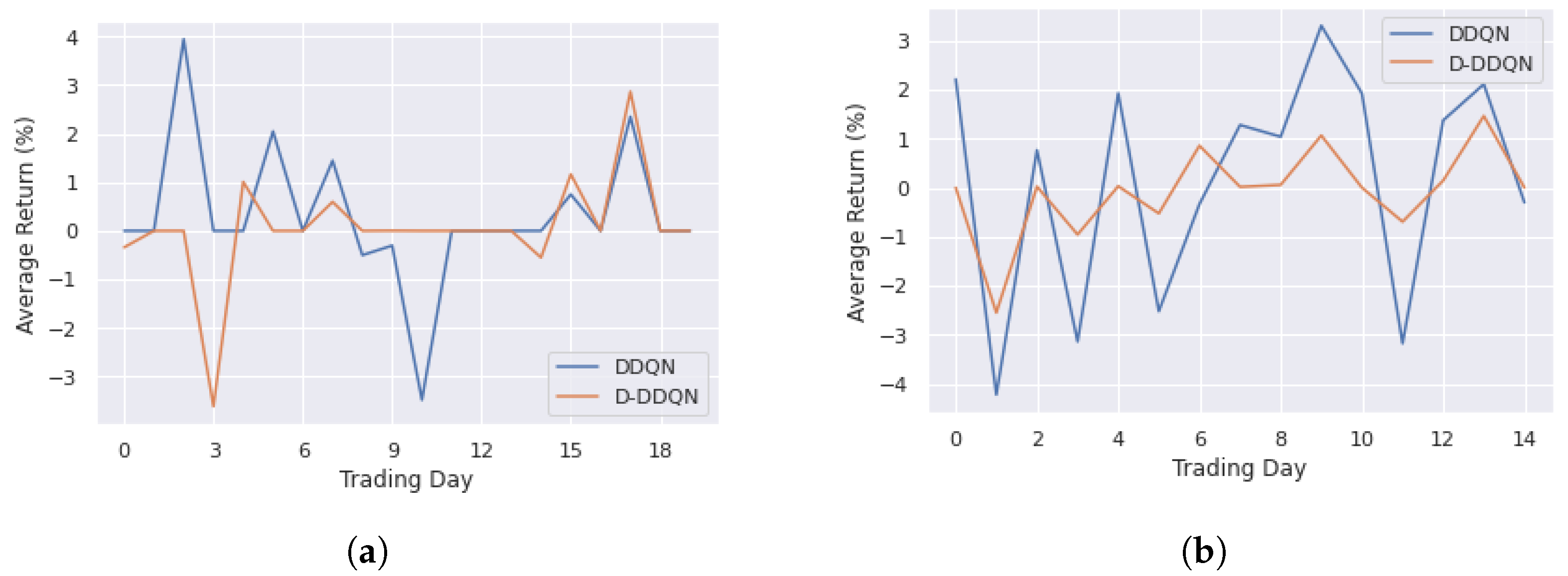
The results with different settings are presented in the tables and figures below. First, the trading system with the cumulative return reward function is considered. In Figure 4a, the average returns in percentage over the training data sets are reported, and the average returns over the 100 testing sets with different start dates and end dates are plotted in Figure 4b. The DDQN setting can beat the D-DDQN setting in terms of return for all the periods; for example, in the training period, DDQN provides the maximum return of 3.95% and maximum loss of −3.48% while the D-DDQN return is 2.87% and loss is −3.61%.
More specifically, Table 3 shows statistical results where the reward function is the cumulative return. Compared with the D-DDQN setting, the system based on DDQN achieves higher average returns in both the training and testing period. However, the standard deviation is also larger, which indicates the instability of the results when trading with short-term periods. In the real market, trading performance is evaluated by the profit achieved after a larger period of time, e.g., weekly or monthly, while this experiment focuses on the daily profit and thus, high volatility is acceptable. In future work, the system could consider different time intervals to compare the stability of the profit achieved.
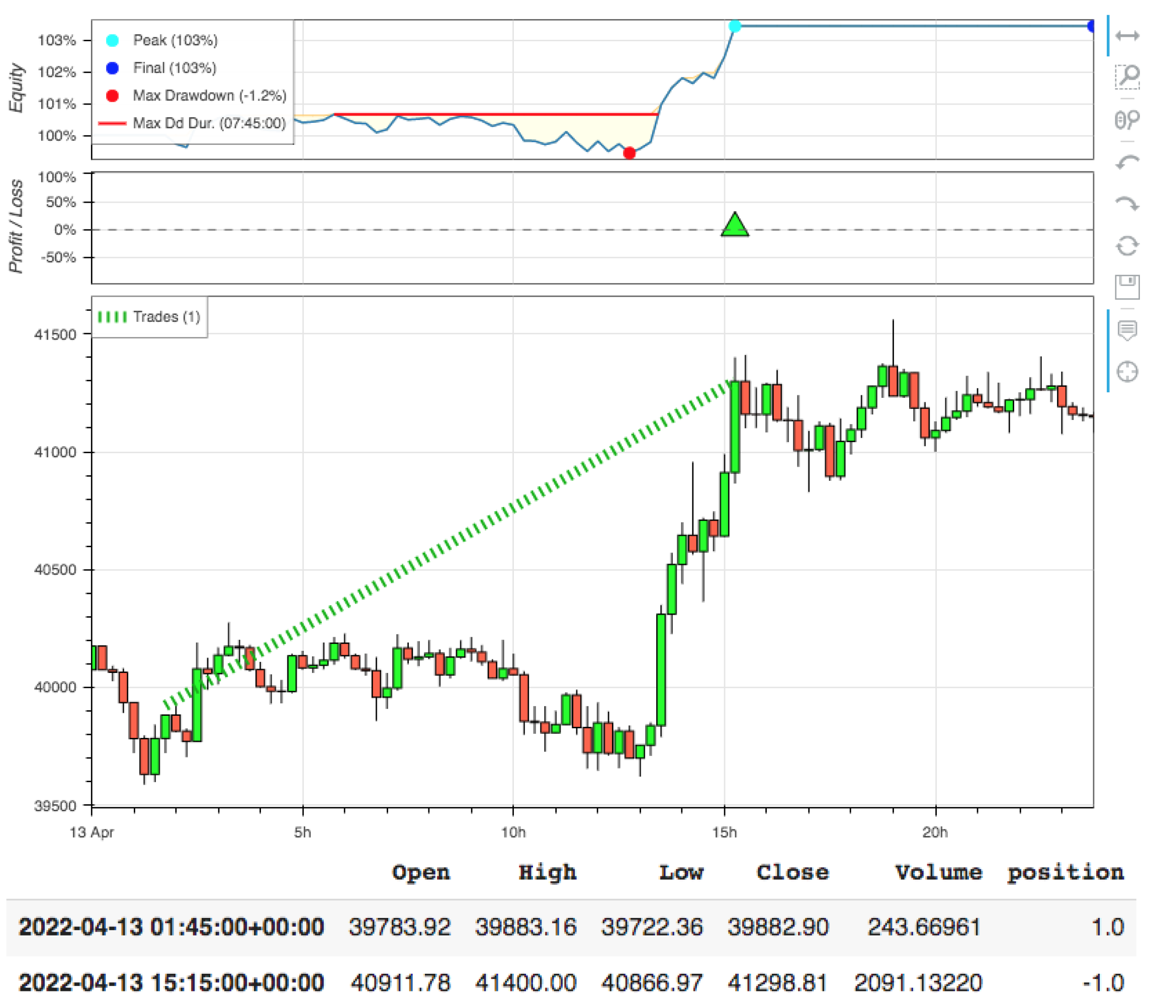
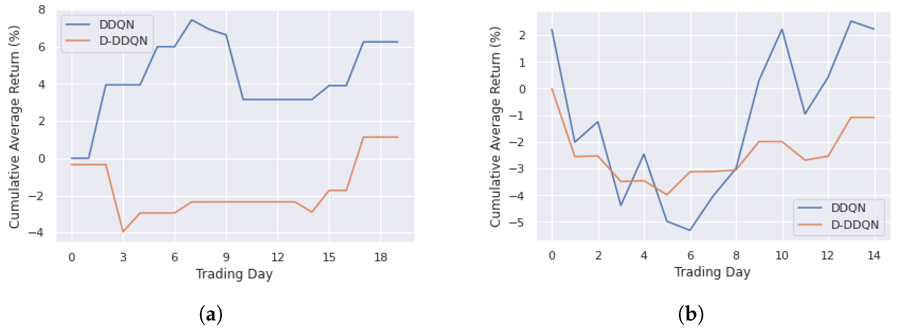
An example of backtesting results and trading details of the trading system in a trading day is shown in Figure 5. To see more clearly the performance of the D-DDQN setting compared with the DDQN setting, we consider the cumulative average returns in all periods. Figure 6a shows the cumulative average return achieved when trading for the entire training period and the performance for the entire testing period is plotted in Figure 6b. The returns of DDQN in the training and testing periods are 6.26% (8.94% per month) and 2.23% (4.46% per month) while the returns of D-DDQN are 1.14% (1.63% per month) and −1.08% (−2.16% per month), respectively. The results show that DDQN setting has better performance than D-DDQN setting with the return reward function.
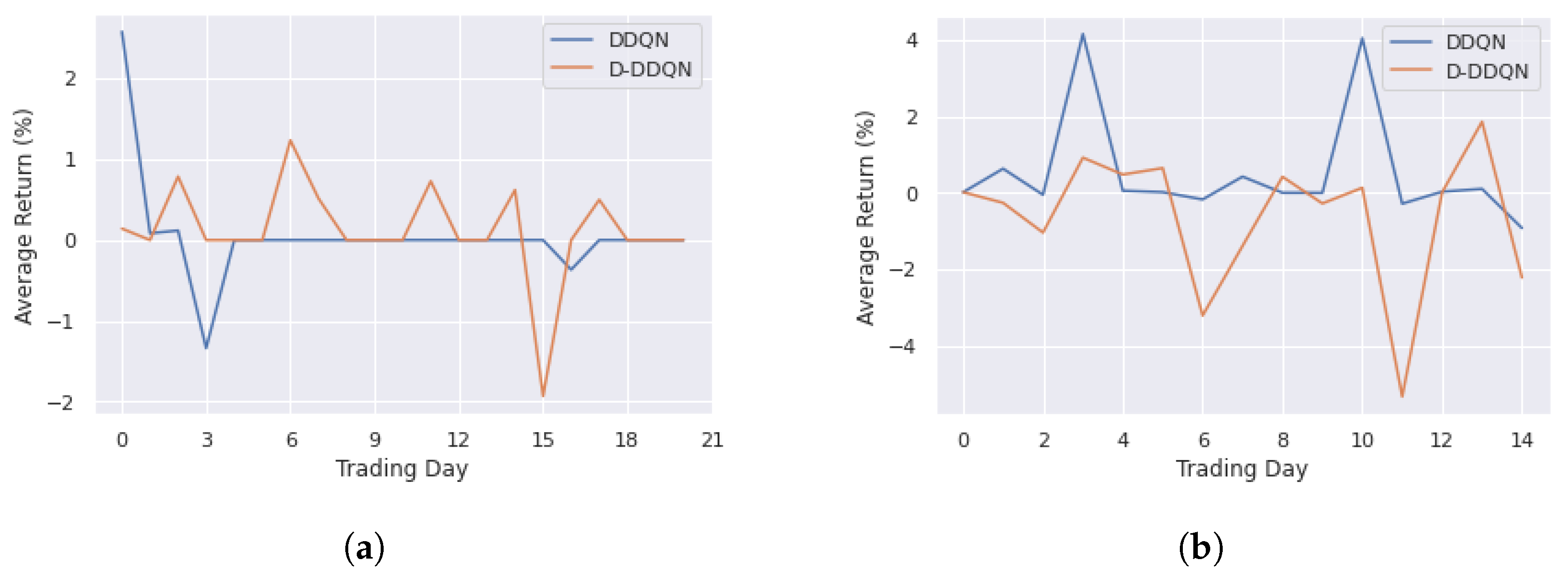
Next, the trading system with the Sharpe reward function is considered. In Figure 7, the average Sharpe value over all the periods is plotted and statistical indicators are summarized in Table 4. Although the D-DDQN setting provides better average returns than DDQN over the training period, other statistical indicators all show that DDQN provides better performance. Furthermore, the DDQN setting provides positive returns and less volatility in all periods.
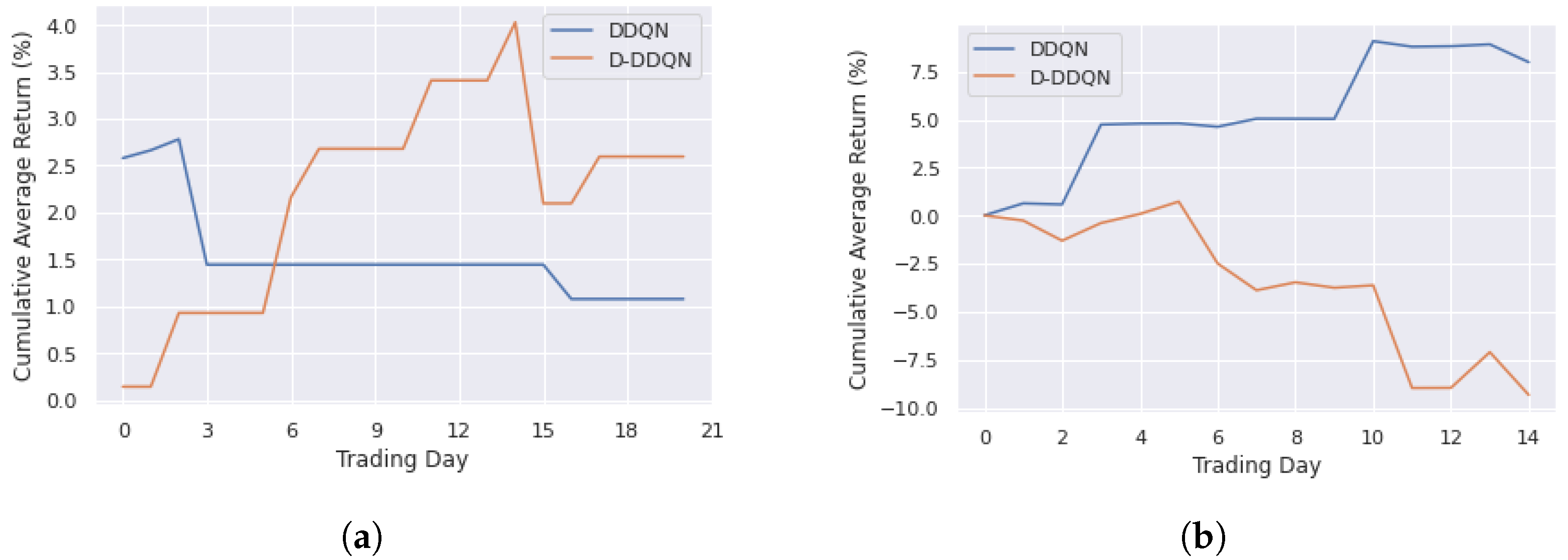
Figure 8a,b report the cumulative average returns over the entire training and testing periods, respectively. The returns of DDQN in the training and testing periods are 1.08% (1.54% per month) and 7.98% (15.96% per month) while the returns of D-DDQN are 2.60% (3.71% per month) and −9.32% (−18.64% per month), respectively. We can see strong fluctuations in the returns of the D-DDQN setting during the training and testing period, whereas DDQN setting provides positive returns in both periods.
From the preliminary analyzes above, the DDQN setting with Sharpe ratio as the reward function proved to be the best Q-learning trading system; this result is consistent with the study in [3].

4.3.2. DRL and Bayesian Optimization Comparision

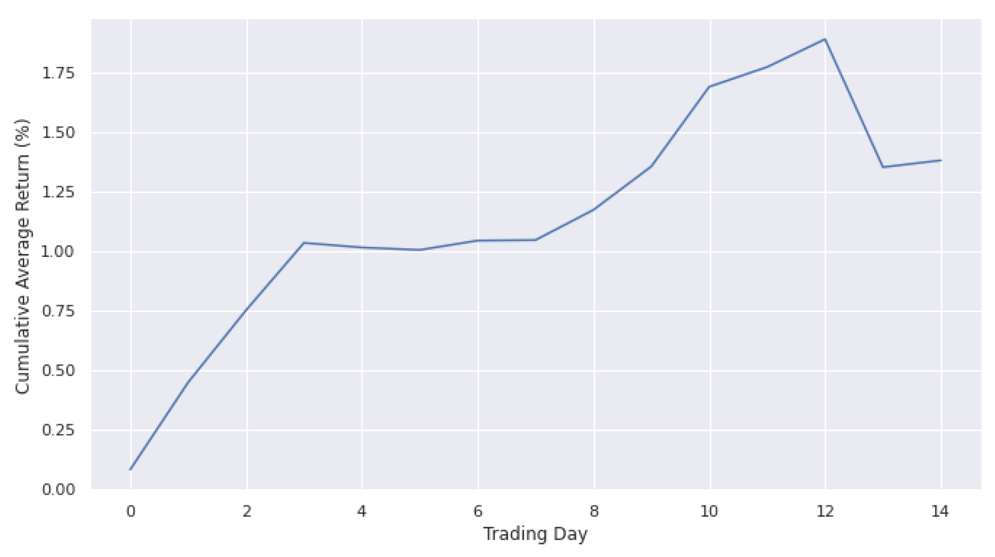
As a benchmark for comparison, the performance of the trading system applying Bayesian Optimization to optimize the strategy is presented in the following figures and tables. The cumulative average return with the return fitness function over 100 testing periods is shown in Figure 9 with a positive return, 1.38%. When compared with the DRL approach, the DDQN setting provides a higher cumulative return (see Figure 6).
Next, Table 5 summarizes the performance of BO approach over 100 different testing sets; the results show that the average return is positive. The highest return is 28.88% and the worst result is −22.45%, which is a big difference indicating the instability of the trading results. The cause of the problem is using only a large data set of the past for training, which is suitable for long-term trading purposes. To solve the problem, the system can regularly update the optimal set of parameters through the rolling training data set, which is consistent with the definition of the DRL approach. Despite using a large data set of the past for training, the system with the DRL setting divides the data into states with each state corresponding to data of a trading day. This means the system takes in new information and updates it to make the best decisions every day. Without loss of generality, the system can be changed to smaller intervals for high frequency purposes.

4.3.3. Execution Time Comparison

Finally, the average execution time for the trading system with different approaches is shown in Table 6. The DRL approach with D-DDQN setting has the shortest execution time. DDQN setting provides smaller volatility than BO approach but it takes longer time to execute. Although DDQN setting could not beat BO in terms of running time in this experiment, the DRL approach still has the potential to outperform BO in practice by looking at better settings with recurrent neural networks. When trading in the real market, traders need to select or combine multiple trading strategies, which creates a large set of parameters that need to be optimized. DRL approach with Deep Q-Network can solve the above challenge while BO meets the problem of high-dimensional domain. Furthermore, the results from BO also show large variability in return performance (see Table 5), so the system needs to be trained continuously as new data sets are added and the validation process should be considered to avoid over-fitting. Let us take an example for this experiment; the system needs to update 100 times to find new optimal parameter sets for 100 different testing sets, and the execution time is doubled when the validation step is included; the total execution time of BO is 2870 s, which is 5.83 times higher than DDQN.

5. Conclusions

This paper presented multiple techniques to optimize the parameters for a trading strategy with RSI indicator. An experiment is carried out with the objective of evaluating the performance of an automated AI trading system with optimized parameters in the framework of Reinforcement Learning. DRL approach with DDQN setting and Bayesian Optimization approach produced positive average returns for high frequency trading purposes. With daily trading goals, the system with DRL approach provided better results when compared to Bayesian Optimization approach. The results also demonstrated that the DDQN setting with Sharpe ratio as the reward function is the best Q-learning trading system. These results provide two options for traders. Traders can apply BO approach with the goal of building a highly profitable trading strategy in the long-term. In contrast, the DRL approach can be applied to regularly update strategies when receiving new information from the market, which helps traders make more effective decisions in short-term trading. The system with DRL settings can also solve the high dimensional problem of parameters of Bayesian Optimization approach; thus, different trading strategies and objective functions as well as new data can be integrated into the system to improve performance.
This research is the first step towards optimizing trading strategies with the Reinforcement Learning framework from popular tools such as Double Deep Q-Network and Dueling Double Deep Q-Network. In future research, the proposed approaches should be compared with recent AI techniques, such as the actor–critic algorithm with deep double recurrent network, for a more accurate comparison study. Another promising approach is to study the impact of financial news on the price movements of cryptocurrencies and incorporate them into automated trading systems.

Author Contributions

Conceptualization, M.T.; formal analysis, M.T.; investigation, M.T.; methodology, M.T.; supervision, D.P.-H. and M.B. All authors have read and agreed to the published version of the manuscript.

Funding

This research received no external funding.

Institutional Review Board Statement

Not applicable.

Informed Consent Statement

Not applicable.

Data Availability Statement

The data are publicly available at https://www.binance.com/en/landing/data, accessed on 1 November 2022.

Conflicts of Interest

The authors declare no conflict of interest.

Abbreviations

The following abbreviations are used in this manuscript:
RLReinforcement learning
DRLDeep reinforcement learning
BOBayesian Optimization
RSIRelative Strength Index
SRSharpe ratio
DDQNDouble Deep Q-Network
D-DDQNDueling Double Deep Q-Network
DNNDeep Neural Network
CNNConvolutional Neural Network

References

  1. Chan, E.P. Quantitative Trading: How to Build Your Own Algorithmic Trading Business; John Wiley & Sons: Hoboken, NJ, USA, 2021. [Google Scholar]
  2. Xiong, Z.; Liu, X.Y.; Zhong, S.; Yang, H.; Walid, A. Practical deep reinforcement learning approach for stock trading. arXiv 2018, arXiv:1811.07522. [Google Scholar]
  3. Lucarelli, G.; Borrotti, M. A deep reinforcement learning approach for automated cryptocurrency trading. In Proceedings of the IFIP International Conference on Artificial Intelligence Applications and Innovations, Crete, Greece, 24–26 May 2019; Springer: Berlin/Heidelberg, Germany, 2019; pp. 247–258. [Google Scholar]
  4. Liu, Y.; Liu, Q.; Zhao, H.; Pan, Z.; Liu, C. Adaptive quantitative trading: An imitative deep reinforcement learning approach. In Proceedings of the AAAI Conference on Artificial Intelligence, New York, NY, USA, 7–12 February 2020; Volume 34, pp. 2128–2135. [Google Scholar]
  5. Ma, C.; Zhang, J.; Liu, J.; Ji, L.; Gao, F. A parallel multi-module deep reinforcement learning algorithm for stock trading. Neurocomputing 2021, 449, 290–302. [Google Scholar] [CrossRef]
  6. Pricope, T.V. Deep reinforcement learning in quantitative algorithmic trading: A review. arXiv 2021, arXiv:2106.00123. [Google Scholar]
  7. Millea, A. Deep reinforcement learning for trading—A critical survey. Data 2021, 6, 119. [Google Scholar] [CrossRef]
  8. Fayek, M.B.; El-Boghdadi, H.M.; Omran, S.M. Multi-objective optimization of technical stock market indicators using gas. Int. J. Comput. Appl. 2013, 68, 41–48. [Google Scholar]
  9. Snoek, J.; Larochelle, H.; Adams, R.P. Practical bayesian optimization of machine learning algorithms. Adv. Neural Inf. Process. Syst. 2012, 25, 2951–2959. [Google Scholar]
  10. Ehrentreich, N. Technical trading in the Santa Fe Institute artificial stock market revisited. J. Econ. Behav. Organ. 2006, 61, 599–616. [Google Scholar] [CrossRef]
  11. Bigiotti, A.; Navarra, A. Optimizing automated trading systems. In Proceedings of the The 2018 International Conference on Digital Science, Budva, Montenegro, 19–21 October 2018; Springer: Berlin/Heidelberg, Germany, 2018; pp. 254–261. [Google Scholar]
  12. Snow, D. Machine learning in asset management—Part 1: Portfolio construction—Trading strategies. J. Financ. Data Sci. 2020, 2, 10–23. [Google Scholar] [CrossRef]
  13. Pardo, R. The Evaluation and Optimization of Trading Strategies; John Wiley & Sons: Hoboken, NJ, USA, 2011; Volume 314. [Google Scholar]
  14. Wu, J.; Chen, X.Y.; Zhang, H.; Xiong, L.D.; Lei, H.; Deng, S.H. Hyperparameter optimization for machine learning models based on Bayesian optimization. J. Electron. Sci. Technol. 2019, 17, 26–40. [Google Scholar]
  15. Bergstra, J.; Bengio, Y. Random search for hyper-parameter optimization. J. Mach. Learn. Res. 2012, 13. [Google Scholar]
  16. Nelder, J.A.; Mead, R. A simplex method for function minimization. Comput. J. 1965, 7, 308–313. [Google Scholar] [CrossRef]
  17. Kirkpatrick, S.; Gelatt, C.D.; Vecchi, M.P. Optimization by simulated annealing. Science 1983, 220, 671–680. [Google Scholar] [CrossRef]
  18. Powell, M.J. A direct search optimization method that models the objective and constraint functions by linear interpolation. In Advances in Optimization and Numerical Analysis; Springer: Berlin/Heidelberg, Germany, 1994; pp. 51–67. [Google Scholar]
  19. Fu, W.; Nair, V.; Menzies, T. Why is differential evolution better than grid search for tuning defect predictors? arXiv 2016, arXiv:1609.02613. [Google Scholar]
  20. Betrò, B. Bayesian methods in global optimization. J. Glob. Optim. 1991, 1, 1–14. [Google Scholar] [CrossRef]
  21. Jones, D.R. A taxonomy of global optimization methods based on response surfaces. J. Glob. Optim. 2001, 21, 345–383. [Google Scholar] [CrossRef]
  22. Ni, J.; Cao, L.; Zhang, C. Evolutionary optimization of trading strategies. In Applications of Data Mining in E-Business and Finance; IOS Press: Amsterdam, The Netherlands, 2008; pp. 11–24. [Google Scholar]
  23. Zhi-Hua, Z. Applications of data mining in e-business and finance: Introduction. Appl. Data Min. E-Bus. Financ. 2008, 177, 1. [Google Scholar]
  24. Jomaa, H.S.; Grabocka, J.; Schmidt-Thieme, L. Hyp-rl: Hyperparameter optimization by reinforcement learning. arXiv 2019, arXiv:1906.11527. [Google Scholar]
  25. Ayala, J.; García-Torres, M.; Noguera, J.L.V.; Gómez-Vela, F.; Divina, F. Technical analysis strategy optimization using a machine learning approach in stock market indices. Knowl.-Based Syst. 2021, 225, 107119. [Google Scholar] [CrossRef]
  26. Fernández-Blanco, P.; Bodas-Sagi, D.J.; Soltero, F.J.; Hidalgo, J.I. Technical market indicators optimization using evolutionary algorithms. In Proceedings of the 10th Annual Conference Companion on Genetic and Evolutionary Computation, Lille, France, 10–14 July 2008; pp. 1851–1858. [Google Scholar]
  27. Théate, T.; Ernst, D. An application of deep reinforcement learning to algorithmic trading. Expert Syst. Appl. 2021, 173, 114632. [Google Scholar] [CrossRef]
  28. Chen, H.H.; Yang, C.B.; Peng, Y.H. The trading on the mutual funds by gene expression programming with Sortino ratio. Appl. Soft Comput. 2014, 15, 219–230. [Google Scholar] [CrossRef]
  29. Kingma, D.P.; Ba, J. Adam: A method for stochastic optimization. arXiv 2014, arXiv:1412.6980. [Google Scholar]
  30. Wilder, J.W. New Concepts in Technical Trading Systems; Trend Research: Greensboro, NC, USA, 1978. [Google Scholar]
  31. Chandra, R.; Goyal, S.; Gupta, R. Evaluation of deep learning models for multi-step ahead time series prediction. IEEE Access 2021, 9, 83105–83123. [Google Scholar] [CrossRef]
  32. Hessel, M.; Modayil, J.; Van Hasselt, H.; Schaul, T.; Ostrovski, G.; Dabney, W.; Horgan, D.; Piot, B.; Azar, M.; Silver, D. Rainbow: Combining improvements in deep reinforcement learning. In Proceedings of the Thirty-Second AAAI Conference on Artificial Intelligence, New Orleans, LA, USA, 2–7 February 2018. [Google Scholar]
  33. Gen, M.; Cheng, R. Genetic Algorithms and Engineering Optimization; John Wiley & Sons: Hoboken, NJ, USA, 1999; Volume 7. [Google Scholar]
  34. Maas, A.L.; Hannun, A.Y.; Ng, A.Y. Rectifier nonlinearities improve neural network acoustic models. In Proceedings of the Icml, Atlanta, GA, USA, 16–21 June 2013; Volume 30, p. 3. [Google Scholar]
  35. Tieleman, T.; Hinton, G. Neural networks for machine learning. Coursera (Lecture-Rmsprop) 2012, 138, 26–31. [Google Scholar]
  36. Duchi, J.; Hazan, E.; Singer, Y. Adaptive subgradient methods for online learning and stochastic optimization. J. Mach. Learn. Res. 2011, 12, 2121–2159. [Google Scholar]
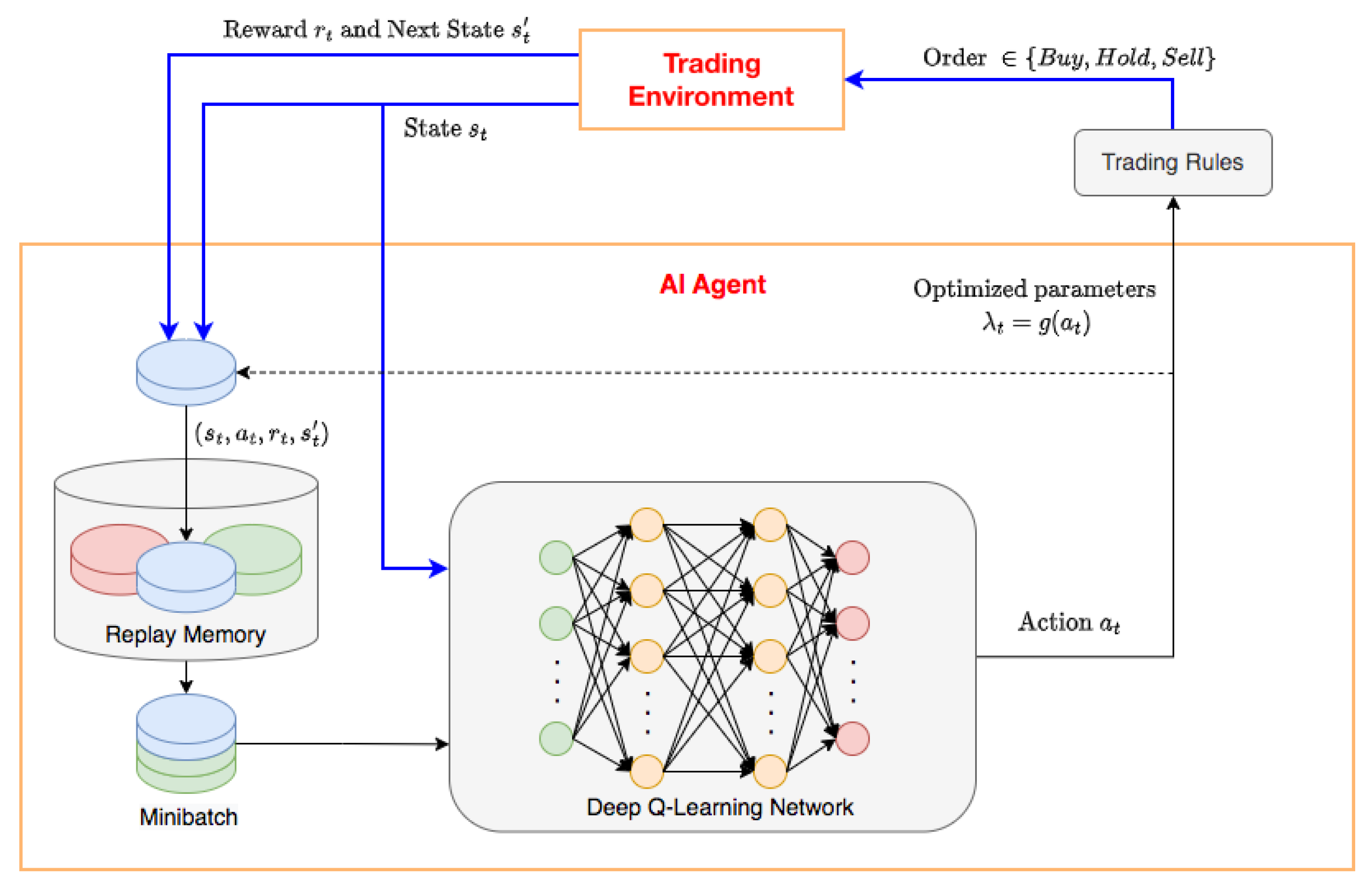
Figure 1. Illustration of the learning mechanism in trading environment.
Algorithms 16 00023 g001
Figure 2. Trend analysis for BTC-USDT closing price.
Algorithms 16 00023 g002
Figure 3. Average price increment ranges by weekday.
Algorithms 16 00023 g003
Figure 4. Average returns from DRL approach with return reward function. (a) Training period; (b) Testing period.
Algorithms 16 00023 g004
Figure 5. Backtesting results of the trading system with DDQN setting.
Algorithms 16 00023 g005
Figure 6. Cumulative average returns from DRL approach with return reward function. (a) Training period; (b) Testing period.
Algorithms 16 00023 g006
Figure 7. Average returns from DRL approach with Sharpe reward function. (a) Training period; (b) Testing period.
Algorithms 16 00023 g007
Figure 8. Cumulative average returns from DRL approach with Sharpe reward function. (a) Training period; (b) Testing period.
Algorithms 16 00023 g008
Figure 9. Cumulative average return performance from BO approach in testing period.
Algorithms 16 00023 g009
Table 1. Summary of the previous research findings on parameter optimization.
Authors (Year)ObjectivesFindings
Ni et al. (2008)
[22]
Discussing evolutionary technologies to
optimize trading strategies
Methods: Genetic Algorithms
Genetic Algorithm approach provides better results in terms
of returns than typical parameters and Buy&Hold strategy.
Genetic Algorithm algorithm can be executed in parallel.
Bergstra & Bengio (2012)
[15]
Comparing different approaches
for neural network optimization
Methods: Random Search, Grid Search,
Manual Search
Random Search on the same domain in high-dimensional
spaces can find better models in less time than Grid Search
and Manual Search.
Snoek et al. (2012)
[9]
Presenting methods to perform BO for
hyperparameter selection of general
machine learning algorithms
Methods: BO with different acquisition
functions
BO with Gaussian Process as probabilistic regression model
and Expected Improvement as acquisition function signifi-
cantly outperforms Tree Parzen Algorithm.
BO surpasses a human expert at selecting hyperparameters
and beats the state of the art by over 3%.
Wu et al. (2019)
[14]
Proposing a hyperparameter tuning
algorithm for machine learning models
Methods: BO, Manual Search
BO algorithm based on Gaussian process can achieve high
accuracy and less running time than Manual Search.
Jomaa et al. (2019)
[24]
Solving hyperparameter optimization
problem with RL approach
Methods: Random Search, BO, RL
The model based on RL approach does not rely on a heuristic
acquisition function like BO. RL method outperforms the
Random Search and BO approaches.
Ayala et al. (2021)
[25]
Optimizing technical analysis strategies
using machine learning
Methods: Grid Search
Linear model and artificial neural network outperform other
machine learning models. The hybrid approach shows
improved profits and reduced risk of losses.
Table 2. Parameters for training the AI agent.
ParametersDescriptionValue
N e Number of episodes100
N B Max capacity of replay memory10,000
b a t c h _ s i z e Batch size40
N u Period of Q target network updates10
γ Discount factor for future rewards0.98
ϵ s t a r t Initial value for epsilon of the ϵ -greedy1
ϵ e n d Final value for epsilon of the ϵ -greedy0.12
l e a r n i n g _ r a t e Learning rate of ADAM optimizer0.001
Table 3. Average return performance with return reward function.
PeriodSettingAvg. (%)Max (%)Min (%)SD.
TrainingDDQN0.313.95−3.481.39
D-DDQN0.062.87−3.611.10
TestingDDQN0.153.30−4.222.26
D-DDQN−0.071.46−2.550.90
Table 4. Average return performance with Sharpe reward function.
PeriodSettingAvg. (%)Max (%)Min (%)SD.
TrainingDDQN0.052.58−1.340.64
D-DDQN0.121.24−1.930.58
TestingDDQN0.534.15−0.931.44
D-DDQN−0.621.8−5.341.76
Table 5. Statistics of average return performance from BO approach.
Avg. Return (%)Max Return (%)Min Return (%)SD.
1.6128.88−22.459.84
Table 6. Execution time for different optimization methods.
MethodExecution Time (s)
DDQN6285
D-DDQN492
BO1435
Disclaimer/Publisher’s Note: The statements, opinions and data contained in all publications are solely those of the individual author(s) and contributor(s) and not of MDPI and/or the editor(s). MDPI and/or the editor(s) disclaim responsibility for any injury to people or property resulting from any ideas, methods, instructions or products referred to in the content.