Article

Adaptive Piecewise Poly-Sinc Methods for Ordinary Differential Equations

1
Mathematics Department, German University in Cairo, New Cairo City 11835, Egypt
2
Department of Mathematics, Faculty of Science, Ain Shams University, Abbassia 11566, Egypt
3
Institute of Applied Analysis and Numerical Simulation, University of Stuttgart, Pfaffenwaldring 57, D-70569 Stuttgart, Germany
4
Faculty of Natural Science, University of Ulm, Albert–Einstein–Allee 11, D-89069 Ulm, Germany
*
Author to whom correspondence should be addressed.
Algorithms 2022, 15(9), 320; https://doi.org/10.3390/a15090320
Submission received: 1 August 2022 / Revised: 5 September 2022 / Accepted: 5 September 2022 / Published: 8 September 2022
(This article belongs to the Special Issue Computational Methods and Optimization for Numerical Analysis)

Abstract

:
We propose a new method of adaptive piecewise approximation based on Sinc points for ordinary differential equations. The adaptive method is a piecewise collocation method which utilizes Poly-Sinc interpolation to reach a preset level of accuracy for the approximation. Our work extends the adaptive piecewise Poly-Sinc method to function approximation, for which we derived an a priori error estimate for our adaptive method and showed its exponential convergence in the number of iterations. In this work, we show the exponential convergence in the number of iterations of the a priori error estimate obtained from the piecewise collocation method, provided that a good estimate of the exact solution of the ordinary differential equation at the Sinc points exists. We use a statistical approach for partition refinement. The adaptive greedy piecewise Poly-Sinc algorithm is validated on regular and stiff ordinary differential equations.

1. Introduction

Numerous phenomena in engineering, physics, and mathematics are modeled either by initial value problems (IVPs) or by boundary value problems (BVPs) described by ordinary differential equations (ODEs). Accordingly, the numerical solution of IVPs for deterministic and random ODEs is a basic problem in the sciences. For a review of the state of the art on theory and algorithms for numerical initial value solvers, we refer to the monographs [1,2,3,4,5,6,7] and the references therein.
Exact solutions may not be available for some ODEs. This has led to the development of a number of methods to estimate the a posteriori error, which is based on the residual of the ODE [8], forming the basis for adaptive methods for ODEs. The a posteriori error estimates have been derived for different numerical methods, such as piecewise polynomial collocation methods [9,10] and Galerkin methods [11,12,13,14]. An a posteriori error estimate in connection with adjoint methods was developed in [15]. Kehlet et al. [16] incorporated numerical round-off errors in their a posteriori estimates. An a posteriori error estimate based on the variational principle was derived in [17]. Convergence rates for the adaptive approximation of ODEs using a posteriori error estimation were discussed in [18,19]. A less common form is the a priori error estimate [8,20]. Hybrid a priori–a posteriori error estimates for ODEs were developed in [21,22]. An advantage of the a priori error estimate over the a posteriori error estimate is that the a priori error estimate does not require the computation of the residual of the ODE. However, some knowledge about the exact solution of the ODE is required for the a priori error estimate. It was shown in [23,24] that the a priori error estimate of the Poly-Sinc approximation is exponentially convergent in the number of Sinc points, provided that the exact solution belongs to the set of analytic functions.
We propose an adaptive piecewise method, in which the points in a given partition are used as partitioning points. This piecewise property allows for a greater flexibility of constructing the polynomials of arbitrary degree in each partition. Recently, we developed an a priori error estimate for the adaptive method based on piecewise Poly-Sinc interpolation for function approximation [25]. In this work [25], we used a statistical approach for partition refinement in which we computed the fraction of a standard deviation [26,27,28] as the ratio of the mean absolute deviation to the sample standard deviation. It was shown in [29] that the ratio approaches 2 π 0.798 for an infinite number of normal samples. We extend the work [25] for regular and stiff ODEs. In this paper, we discuss the adaptive piecewise Poly-Sinc method for regular and stiff ODEs, and show that the exponentially convergent a priori error estimate for our adaptive method differs from that for function approximation [25] by a small constant.
This paper is organized as follows. Section 2 provides an overview of the Poly-Sinc approximation, the residual computation, the indefinite integral approximation, and the collocation method. Section 3 discusses the piecewise collocation method, which is the cornerstone of the adaptive piecewise Poly-Sinc algorithm. In Section 4, we present the adaptive piecewise Poly-Sinc algorithm for ODEs and the statistical approach for partition refinement. We also demonstrate the exponential convergence of the a priori error estimate for our adaptive method. We validate our adaptive Poly-Sinc method on regular ODEs and ODEs whose exact solutions exhibit an interior layer, a boundary layer, and a shock layer in Section 5. Finally, we present our concluding remarks in Section 6.

2. Background

2.1. Poly-Sinc Approximation

A novel family of polynomial approximation called Poly-Sinc interpolation which interpolate data of the form { x k , y k } k = M N where { x k } k = M N are Sinc points, were derived in [23,30] and extended in [24]. The interpolation to this type of data is accurate provided that the function y with values y k = y ( x k ) belong to the space of analytic functions [30,31]. For the ease of presentation and discussion, we assume that M = N . Poly-Sinc approximation was developed in order to mitigate the poor accuracy associated with differentiating the Sinc approximation when approximating the derivative of functions [23]. Moreover, Poly-Sinc approximation is characterized by its ease of implementation. Theoretical frameworks on the error analysis of function approximation, quadrature, and the stability of the Poly-Sinc approximation were studied in [23,24,32,33]. Furthermore, Poly-Sinc approximation was used to solve BVPs in ordinary and partial differential equations [31,34,35,36,37,38]. We start with a brief overview of Lagrange interpolation. Then, we discuss the generation of Sinc points using conformal mappings.

2.1.1. Lagrange Interpolation

Lagrange interpolation is a polynomial interpolation scheme [39], which is constructed by Lagrange basis polynomials
u k ( x ) = g ( x ) ( x x k ) g ( x k ) , k = 1 , 2 , , m ,
where { x k } k = 1 m are the interpolation points and g ( x ) = l = 1 m ( x x l ) . The Lagrange basis polynomials satisfy the property
u k ( x j ) = { 1 , if   k = j , 0 , if   k j .
Hence, the polynomial approximation in the Lagrange form can be written as
y h ( x ) = k = 1 m y ( x k ) u k ( x ) ,
where y h ( x ) is a polynomial of degree m 1 and it interpolates the function f ( x ) at the interpolation points, i.e., y h ( x k ) = y ( x k ) . For Sinc points, the polynomial approximation y h ( x ) becomes
y h ( x ) = k = N N y ( x k ) u k ( x ) ,
where m = 2 N + 1 is the number of Sinc points. If the coefficients y ( x k ) are unknown, then we replace y ( x k ) with c k , and Equations (1) and (2) become
y c ( x ) = k = 1 m c k u k ( x )
and
y c ( x ) = k = N N c k u k ( x ) ,
respectively.

2.1.2. Conformal Mappings and Function Space

We introduce some notations related to Sinc methods [23,24,30]. Let φ : D D d be a conformal map that maps a simply connected region D C onto the strip
D d = { z C : | Im ( z ) | < d } ,
where d is a given positive number. The region D has a boundary D , and let a and b be two distinct points on D . Let ψ = φ 1 , ψ : D d D be the inverse conformal map. Let Γ be an arc defined by
Γ = { z [ a , b ] : z = ψ ( x ) , x R } ,
where a = ψ ( ) and b = ψ ( ) . For real finite numbers a , b , and Γ R , φ ( x ) = ln ( ( x a ) / ( b x ) ) and x k = ψ ( k h ) = ( a + b e k h ) / ( 1 + e k h ) are the Sinc points with spacing h ( d , β s ) = π d β s N 1 / 2 , β s > 0  [30,40]. Sinc points can be also generated for semi-infinite or infinite intervals. For a comprehensive list of conformal maps, see [24,30].
We briefly discuss the function space for y. Let ρ = e φ , α s be an arbitrary positive integer number, and L α s , β s ( D ) be the family of all functions that are analytic in D = φ 1 ( D d ) such that for all z D , we have
| y ( z ) | C | ρ ( z ) | α s [ 1 + | ρ ( z ) | ] α s + β s .
We next set the restrictions on α s , β s , and d such that 0 < α s 1 , 0 < β s 1 , and 0 < d < π . Let M α s , β s ( D ) be the set of all functions g defined on D that have finite limits g ( a ) = lim z a g ( z ) and g ( b ) = lim z b g ( z ) , where the limits are taken from within D, and such that y L α s , β s ( D ) , where
y = g g ( a ) + ρ g ( b ) 1 + ρ .
The transformation guarantees that y vanishes at the endpoints of ( a , b ) . We assume that y is analytic and uniformly bounded by B ( y ) , i.e.,  | y ( x ) | B ( y ) , in the larger region
D 2 = D t ( a , b ) B ( t , r ) ,
where r > 0 and B ( t , r ) = { z C : | z t | < r } .

2.2. Residual

The residual is used as a measure of the accuracy of the adaptive Poly-Sinc method. The general form of a second-order ODE can be expressed as [41]
F ( x , y , y , y ) = 0 .
An exact solution y satisfies (5). If the exact solution y is unknown, we replace it with the approximation y c and Equation (5) becomes
F ( x , y c , y c , y c ) = R ( x ) ,
where R ( x ) is the residual. The residual in (6) for the i th iteration becomes
F x , y c ( i ) , y c ( i ) , y c ( i ) = R ( i ) ( x ) , i = 1 , 2 , , κ ,
where κ is the number of iterations.
We will denote the residual for integral and differential equations with R I and R D , respectively. The residual is used as an indicator for partition refinement as discussed in Algorithm 4 (see Section 4).

2.3. Error Analysis

We briefly discuss the error analysis for Poly-Sinc approximation over the global interval [ a , b ] . At the end of this section, we will discuss the error analysis of Poly-Sinc approximation for IVPs and BVPs.
For the Poly-Sinc approximation on a finite interval [23,24,32,33,38], it was shown that
max x [ a , b ] | y ( x ) y h ( x ) | A r m N e β N ,
where y ( x ) is the exact solution and y h ( x ) is its Poly-Sinc approximation, A is a constant independent of N, m = 2 N + 1 is the number of Sinc points in the interval, r is the radius of the ball containing the m Sinc points, and β > 0 is the convergence rate parameter. On a finite interval [ a , b ] , it was shown that [24,38]
max x [ a , b ] | y ( x ) y h ( x ) | A b a 2 r m N 3 / 2 tanh [ 4 ] ( η 4 N ) exp ( π 2 N 2 η ) ,
where η is a positive constant. Inequality (7) can be written as
max x [ a , b ] | y ( x ) y h ( x ) | A b a 2 r m N α exp ( γ N β ) .
Next, we discuss the collocation method for IVPs and BVPs.

2.4. Collocation Method

A collocation method [42,43] is a technique in which a system of algebraic equations is constructed from the ODE via the use of collocation points. Here, we adopt the Poly-Sinc collocation method [36,44], in which the collocation points are the Sinc points and the basis functions are the Lagrange polynomials with Sinc points.

2.4.1. Initial Value Problem

The IVP is transformed into an integral equation. We briefly discuss the approximation of indefinite integrals using Poly-Sinc methods ([45] § 9.3). Define
( J + w y ) ( x ) = a x y ( t ) w ( t ) t ,
where the weight function w ( x ) is positive on the interval ( a , b ) and has the property that the moments a b x j w ( x ) x do not vanish for j = 0 , 1 , 2 , . Let A + be an m × m matrix whose entries are
[ A + ] k j = a x k u j ( x ) w ( x ) x ,
where u j ( x ) , j = N , , N , are the Lagrange basis polynomials stacked in a vector L ( x ) = ( u N ( x ) , , u N ( x ) ) , and ( · ) is the transpose operator. The interpolation points { x j } j = N N are the Sinc points generated in the interval [ a , b ] as discussed in Section 2.1.2.
Then, the indefinite integral (8) can be approximated as
( J m + w y ) ( x ) = j = N N ( J m + w y ) ( x j ) u j ( x ) j = N N k = N N y ( x k ) [ A + ] j k u j ( x ) = j = N N u j ( x ) k = N N y ( x k ) [ A + ] j k = L ( x ) A + V y ,
where V y = ( y ( x N ) , , y ( x N ) ) . We state the following theorem for IVPs [30].
Theorem 1 
(Initial Value Problem ([30] §1.5.8)). If y M α s , β s ( D ) , then, for all N > 1
J + w y J m + w y = O ( ϵ N ) ,
where ϵ N = N e β N .

2.4.2. Boundary Value Problem

For a BVP, the collocation method solves for the unknown coefficients c k in (3) or (4) by setting
R D ( x k ) = 0 , k = N , , N .
However, we replace the two equations corresponding to x N and x N with the boundary conditions y ( a ) = y a and y ( b ) = y b , respectively. We state the following theorem for BVPs.
Theorem 2 
(Boundary Value Problem ([30] §1.5.6)). If y M α s , β s ( D ) and c = ( c N , , c N ) is a complex vector of order m, such that for some δ > 0 ,
j = N N y ( x j ) c j 2 1 / 2 < δ ,
then,
y L ( x ) c < C ϵ N + δ .

3. Piecewise Collocation Method

We discuss the piecewise collocation method, in which the domain I = [ a , b ] is discretized into K N non-overlapping partitions I n = [ x n 1 , x n ) , n = 1 , 2 , , K 1 , x 0 = a , x K = b with I K = [ x K 1 , b ] and n = 1 K I n = I = [ a , b ] . The space of piecewise discontinuous polynomials can be defined as
D k ( I ) = { v : v | I n P k ( I n ) , n = 1 , 2 , , K } ,
where P k ( I n ) denotes the space of polynomials of degree at most k on I n . The piecewise collocation method solves the collocation method in Section 2.4 over partitions. The approximate solution in the global partition [ a , b ] can be written as
y h ( x ) = k = 1 K y h , k ( x ) 1 x I k = k = 1 K 1 x I k j = 1 m k y j , k u j , k ( x ) ,
where y h , k ( x ) = j = 1 m k y j , k u j , k ( x ) is the Lagrange interpolation in the k th partition. The basis functions
u j , k ( x ) = g k ( x ) ( x x j , k ) g k ( x j , k ) , j = 1 , 2 , , m k , k = 1 , 2 , K ,
where { x j , k } j = 1 m k are the interpolation points in the k th partition, g k ( x ) = l = 1 m k ( x x l , k ) , and m k is the number of points in the k th partition. The function 1 C is an indicator function which outputs 1 if the condition C is satisfied and otherwise 0. If the coefficients y j , k are unknown, then we replace y j , k with c j , k , and Equation (9) becomes
y c ( x ) = k = 1 K y c , k ( x ) 1 x I k = k = 1 K 1 x I k j = 1 m k c j , k u j , k ( x ) .
The residual for the k th partition can be written as
F x , y c , k , y c , k , y c , k = R k ( x ) , x I k , k = 1 , 2 , , K .
The collocation method solves for the unknowns c j , k by setting R k ( x j , k ) = 0 , j = 1 , 2 , , m k , k = 1 , 2 , , K , which we discuss next for IVPs and BVPs.

3.1. Initial Value Problem

In this section, we provide examples for first-order and second-order IVPs.

Relaxation Problem

We discuss the piecewise collocation method for a first-order IVP in integral form. Consider the following relaxation or decay Equation [46] on the interval [ a , b ]
y ( x ) x = α y ( x ) , y ( a ) = y a ,
where α > 0 is the relaxation parameter. The exact solution is y ( x ) = y a exp ( α ( x a ) ) . We transform the IVP (11) into an integral form
y ( x ) = y a α a x y ( t ) t .
The residual becomes
R I ( x ) = y c ( x ) y a + α a x y ( t ) t .
We approximate the indefinite integral as discussed in Section 2.4.1 and the approximate residual becomes
R ˜ I ( x , a , y a , y c ( x ) ) = y c ( x ) y a + α ( J m + y c ) ( x ) .
The domain [ a , b ] is partitioned as discussed in Section 3. For the k th partition, k = 1 , 2 , , K , we replace a with x k 1 and y a with y c , k 1 ( x k 1 ) . The approximate residual becomes
R ˜ I , k ( x , x k 1 , y c , k 1 ( x k 1 ) , y c , k ( x ) ) = y c , k ( x ) y c , k 1 ( x k 1 ) + α ( J m + y c ) ( x ) , x I k .
We remove the equation corresponding to the leftmost Sinc point in each partition, and replace them with the conditions
y c ( x 0 ) = y a ,
y c , k ( x k 1 ) = y c , k 1 ( x k 1 ) , k = 2 , 3 , , K ,
and the set of equations
R ˜ I , k ( x j , k , x k 1 , y c , k 1 ( x k 1 ) , y c , k ( x j , k ) ) = 0 , j = 2 , 3 , , m k , k = 1 , 2 , , K .
The set of equations (12b) is known as the continuity equations at the interior boundaries [47]. The collocation algorithm for the IVP (11) is outlined in Algorithm 1.
Algorithm 1: Piecewise Poly-Sinc Algorithm (IVP (11)).
input K : number of partitions
       m k : number of Sinc points in the k th partition
output y c ( x ) : approximate solution
 Replace y ( x ) with the global approximate solution (10).
 Solve for the m k K unknowns { c j , k } j = 1 , k = 1 m k , K using the initial condition (12a),
 continuity Equation (12b), and the set of equations for the residual (13).

3.2. Hanging Bar Problem

We discuss the piecewise collocation method for a second-order IVP in integral form. Considering the following IVP on the interval [ a , b ]
x a , b , ( K ˜ ( x ) y ( x ) ) = f ( x ) , y ( a ) = y a , y ( a ) = y ˜ a .
where y ( x ) is the sought-for solution. In the context of the hanging bar problem [48], y ( x ) and K ˜ ( x ) are the displacement and the material property of the bar at the position x, respectively. For simplicity, we set K ˜ ( x ) = 1 . Equation (14) can be written as a system of first-order equations
y = q , q = f , y ( a ) = y a , q ( a ) = y ˜ a .
The integral form of (15) is
y ( x ) = y a + a x q ( t ) t ,
q ( x ) = y ˜ a a x f ( t ) t .
Plugging (17) into (16), we obtain
y ( x ) = y a + a x y ˜ a a t f ( s ) s t = y a + y ˜ a ( x a ) a x a t f ( s ) s t .
Using integration by parts u v = u v v u  [49] with u ( t ) = a t f ( s ) s ,
a x a t f ( s ) s t = t a t f ( s ) s | t = a t = x a x t f ( t ) t = x a x f ( s ) s a x t f ( t ) t = x a x f ( s ) s a x s f ( s ) s = a x ( x s ) f ( s ) s ,
where we set t = s . Thus, the integral form of the solution to (14) becomes
y ( x ) = y a + ( x a ) y ˜ a x a x f ( s ) s + a x s f ( s ) s .
The residual can be written as
R I ( x , a , y a , y ˜ a , y c ( x ) ) = y c ( x ) y a ( x a ) y ˜ a + x a x f ( s ) s a x s f ( s ) s .
Approximating the indefinite integral in (18), the approximate residual becomes
R ˜ I ( x , a , y a , y ˜ a , y c ( x ) ) = y c ( x ) y a ( x a ) y ˜ a + x ( J m + f ) ( x ) ( J m + x f ) ( x ) .
For the k th partition, k = 1 , 2 , , K , we replace a with x k 1 , y a with y c , k 1 ( x k 1 ) , and y ˜ a with y c , k 1 ( x k 1 ) . The approximate residual becomes
R ˜ I , k ( x , x k 1 , y c , k 1 ( x k 1 ) , y c , k 1 ( x k 1 ) , y c , k ( x ) ) = y c , k ( x ) y c , k 1 ( x k 1 ) ( x x k 1 ) y c , k 1 ( x k 1 ) + x ( J m + f ) ( x ) ( J m + x f ) ( x ) , x I k .
We remove the equations corresponding to the leftmost and rightmost Sinc points in each partition, and replace them with the conditions
y c ( x 0 ) = y a ,
y c ( x 0 ) = y ˜ a ,
y c , k ( x k 1 ) = y c , k 1 ( x k 1 ) , k = 2 , , K ,
and the set of equations
R ˜ I , k ( x j , k , x k 1 , y c , k 1 ( x k 1 ) , y c , k 1 ( x k 1 ) , y c , k ( x j , k ) ) = 0 ,
j = 2 , , m k 1 , k = 1 , , K . Equations (20c)–(20d) are known as the continuity equations at the interior boundaries [47]. The collocation algorithm for the IVP (14) is outlined in Algorithm 2.
Algorithm 2: Piecewise Poly-Sinc Algorithm (IVP (14)).
input K : number of partitions
       m k : number of Sinc points in the k th partition
output y c ( x ) : approximate solution
 Replace y ( x ) with the global approximate solution (10).
 Solve for the m k K unknowns { c j , k } j = 1 , k = 1 m , K using initial conditions (20a)–(20b),
 continuity Equations (20c)–(20d), and the set of equations for the residual (21).

3.3. Boundary Value Problem

The collocation method for the BVP is similar to that of the IVP in Section 3.2, except that we replace the set of equations (20) with
y c ( x 0 ) = y a ,
y c ( x K ) = y b ,
y c , k ( x k 1 ) = y c , k 1 ( x k 1 ) , k = 2 , 3 , , K ,
and the set of equations of the residual for the BVP becomes
R D , k ( x j , k ) = 0 , j = 2 , 3 , , m k 1 , k = 1 , 2 , , K ,
where R D , k is the residual of the differential equation in the k th partition. The piecewise Poly-Sinc collocation algorithm for the BVP is outlined in Algorithm 3.
Algorithm 3: Piecewise Poly-Sinc Algorithm (BVP).
input K : number of partitions
       m k : number of Sinc points in the k th partition
output y c ( x ) : approximate solution
 Replace y ( x ) with the global approximate solution (10).
 Solve for the m k K unknowns { c j , k } j = 1 , k = 1 m , K using boundary conditions (22a)–(22b), continuity Equations (22c)–(22d), and the set of equations for the residual (23).

4. Adaptive Piecewise Poly-Sinc Algorithm

This section introduces the greedy algorithmic approach used in adaptive piecewise Poly-Sinc methods. The core feature used is the non-overlapping properties of Sinc points and the uniform exponential convergence on each partition of the approximation interval. Greedy algorithms seek the “best” candidate of possible solutions at a given step [50]. Greedy algorithms have been applied to model order reduction for parametrized partial differential equations [51,52]. The adaptive piecewise Poly-Sinc algorithm is greedy in the sense that it makes a choice that aims to find the “best” approximation for the solution of the ODE in the current step [50]. The algorithm takes an iterative form in which it computes the L 2 norm values of the residual for all partitions constituting the global interval I = [ a , b ] . At the i th step, the algorithm refines the partitions for which the L 2 norm values of the residual are relatively large. By refining the partitions as discussed above, it is expected that the mean value of the L 2 norm values over all partitions decreases in each step. As the iteration proceeds, the algorithm expects to find the “best” polynomial approximation for the solution of the ODE.

4.1. Algorithm Description

We discuss the adaptive algorithm for the piecewise Poly-Sinc approximation. The following steps of the adaptive algorithm are performed in an iterative loop [53]
SOLVE ESTIMATE MARK REFINE .
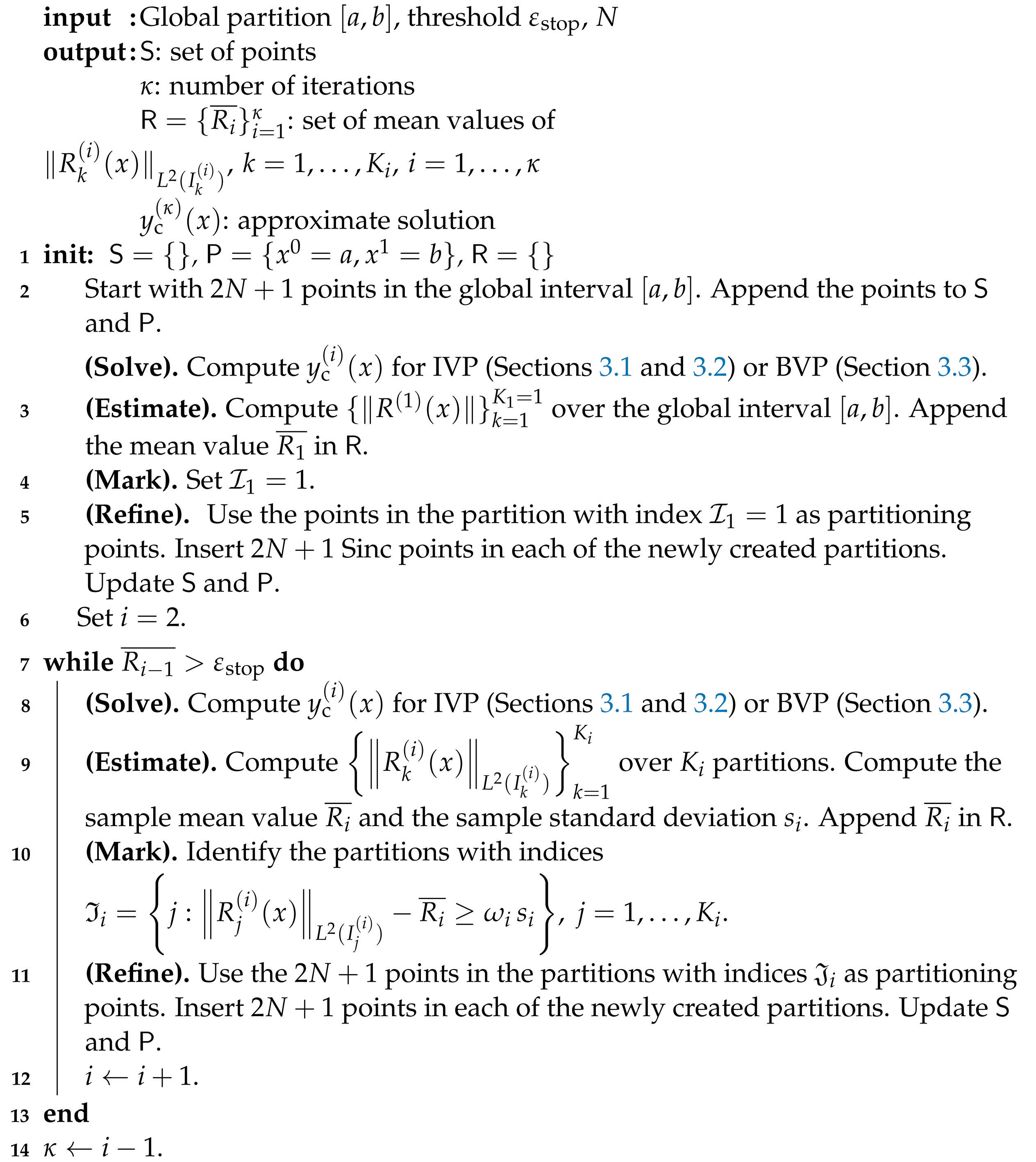
The adaptive piecewise Poly-Sinc algorithm is outlined in Algorithm 4. The refinement strategy is performed as follows. For the i th iteration, we compute the set of L 2 norm values R k ( i ) ( x ) L 2 ( I k ( i ) ) k = 1 K i over the K i partitions, from which the sample mean R i ¯ = 1 K i j = 1 K i R j ( i ) ( x ) L 2 ( I j ( i ) ) and the sample standard deviation [54]
s i = 1 K i 1 j = 1 K i R j ( i ) ( x ) L 2 ( I j ( i ) ) R i ¯ 2
are computed [26,27,28]. The residual R j ( i ) ( x ) for the j th partition and the i th iteration is discussed in Section 2.2. The partitions with the indices I i = j : R j ( i ) ( x ) L 2 ( I j ( i ) ) R i ¯ ω i s i are marked for refinement, where the statistic [29]
ω i = 1 K i j = 1 K i R j ( i ) ( x ) L 2 ( I j ( i ) ) R i ¯ s i .
Using Hölder’s inequality for sums with p = q = 2  ([55] § 3.2.8), one can show that ω i K i 1 K i < 1 . We restrict to second-order moments only. The points in the partitions with the indices I i are used as partitioning points and m = 2 N + 1 Sinc points are inserted in the newly created partitions. The algorithm terminates when the stopping criterion is satisfied. The approximate solution y c ( i ) ( x ) , i = 1 , , κ , for the i th iteration is computed using the collocation method outlined in Algorithms 1 and 2 for IVPs and Algorithm 3 for BVPs. We note that, for partition refinement, the residual is computed in its differential form R D ( x ) .
The definite integral in the L 2 norm [56] is numerically computed using a Sinc quadrature [30], i.e.,
f ( x ) L 2 ( [ a , b ] ) 2 = a b | f ( x ) | 2 x h k = N N 1 φ ( x k ) f 2 ( x k ) ,
where { x k } k = N N [ a , b ] are the quadrature points, which are also Sinc points, and φ ( x ) is the conformal mapping in Section 2.1.2. The supremum norm on an interval I = [ a , b ] is approximated as ([57] Table 2.1)
f ( x ) I max { | f ( x k ) | } k = N N ,
where { x k } k = N N are the Sinc points on I, whose generation is discussed in Section 2.1.2.

4.2. Error Analysis

We state below the main theorem.
Theorem 3
(Estimate of Upper Bound [25]). Let y be in M α s , β s ( φ ) , analytic and bounded in D 2 , and let y h ( i ) ( x ) be the piecewise Poly-Sinc approximation in the i-th iteration. Let ξ i = arg max k Len ( I k ( i ) ) be the index of the largest partition in the i th iteration and Len ( I k ( i ) ) be the length of the k th partition in the i th iteration. Let K i be the number of partitions in the i th iteration. Then, there exists a constant A, independent of the i th iteration, such that
max x [ a , b ] y ( x ) y h ( i ) ( x ) K i E i ,
where E i = A ( 2 r ξ i ) m ξ i λ m ξ i ( i 1 ) ( b a ) m ξ i .
For fitting purposes, we compute the mean value of the error estimate, i.e.,
max x [ a , b ] 1 K i y ( x ) y h ( i ) ( x ) E i .
We state the following theorem on collocation.
Algorithm 4: Adaptive Piecewise Poly-Sinc Algorithm.
Algorithms 15 00320 i001
Theorem 4.
Let y be in M α s , β s ( φ ) , analytic and bounded in D 2 , and let y c ( i ) ( x ) be the piecewise Poly-Sinc approximation in the i-th iteration with the estimated coefficients c j , k ( i ) using the piecewise collocation method in Section 3. Let m k ( i ) be the number of points in the k th partition for the i th iteration and n i = k = 1 K i m k ( i ) be the total number of points in the i th iteration. Let c i = ( c 1 , 1 ( i ) , , c 1 , m 1 ( i ) ( i ) , , c 1 , K i ( i ) , , c 1 , m K i ( i ) ( i ) ) be the n i × 1 vector of estimated coefficients in y c ( i ) ( x ) and y i = y ( x j , k ( i ) ) be the corresponding vector of the exact values of y ( x ) at the Sinc points { x j , k ( i ) } with
c i y i 1 < δ , i = 1 , 2 , , κ .
Then,
max x [ a , b ] | y ( x ) y c ( i ) ( x ) | K i E i + δ 1 π ln ( m ¯ ¯ ) + 1.07618 ,
where m ¯ ¯ = max k , i { m k ( i ) } and · 1 denotes the 1 norm ([58] Ch. 5).
Proof. 
The derivation follows that of ([30] § 1.5.6).
max x [ a , b ] | y ( x ) y c ( i ) ( x ) | = y ( x ) y c ( i ) ( x ) I = y ( x ) y c ( i ) ( x ) + y h ( i ) ( x ) y h ( i ) ( x ) I y ( x ) y h ( i ) ( x ) I + y c ( i ) ( x ) y h ( i ) ( x ) I y ( x ) y h ( i ) ( x ) I + k = 1 K i 1 x I k ( i ) j = 1 m k ( i ) ( c j , k ( i ) y j , k ( i ) ) u j , k ( i ) ( x ) I K i E i + k = 1 K i j = 1 m k ( i ) ( c j , k ( i ) y j , k ( i ) ) u j , k ( i ) ( x ) I k ( i ) K i E i + k = 1 K i j = 1 m k ( i ) | c j , k ( i ) y j , k ( i ) | · | u j , k ( i ) ( x ) | I k ( i ) K i E i + δ K i k = 1 K i j = 1 m k ( i ) | u j , k ( i ) ( x ) | I k ( i ) K i E i + δ K i k = 1 K i 1 π ln ( m k ( i ) ) + 1.07618 K i E i + δ K i K i 1 π ln ( m ¯ ¯ ) + 1.07618 = K i E i + δ 1 π ln ( m ¯ ¯ ) + 1.07618 ,
where j = 1 m k ( i ) | u j , k ( i ) ( x ) | I k ( i ) 1 π ln ( m k ( i ) ) + 1.07618 is the Lebesgue constant for Poly-Sinc approximation [31,33,59]. On average, the term | c j , k ( i ) y j , k ( i ) | < δ n i < δ K i min k { m k ( i ) } < δ K i . □
For fitting purposes, we compute the mean value of the error estimate, i.e.,
max x [ a , b ] 1 K i y ( x ) y c ( i ) ( x ) E i + δ K i 1 π ln ( m ¯ ¯ ) + 1.07618 < E i + δ 1 π ln ( m ¯ ¯ ) + 1.07618 .

5. Results

The results in this section were computed using Mathematica [60]. We tested our adaptive algorithm on regular and stiff ODEs. The Sinc spacing is h = π e N . For all examples, we set e = 1 / 2 and the number of points per partition to be constant, i.e., m k ( i ) = m = 2 N + 1 . A precision of 200 digits is used.

5.1. Norms

The supremum norm has a theoretical advantage. However, its computation is slower than that of the L 2 norm [25]. Hence, we use the L 2 norm in our computations.

5.2. Initial Value Problem

We test our adaptive piecewise Poly-Sinc algorithm on regular first-order and second-order IVPs.
Example 1
(Relaxation Problem). We start with the relaxation problem in Section 3.1. We set a = 0 and the exact solution becomes y ( x ) = exp ( α x ) . We set the exponential decay parameter α = 20 and confine the domain of the solution to the interval [ 0 , 1 ] . The approximate solution y c ( x ) is computed as discussed in Section 3.1.
We set the number of Sinc points to be inserted in all partitions as m = 2 N + 1 = 5 . The stopping criterion ε stop = 10 6 was used. The algorithm terminates after κ = 7 iterations and the number of points | S | = 530 .
Figure 1a shows the approximate solution y c ( 7 ) ( x ) . A proper subset of the set of points S is shown as red dots, which are projected onto the approximate solution y c ( 7 ) ( x ) . This proper subset is used to observe the approximate solution y c ( 7 ) ( x ) . We plot the statistic ω i as a function of the iteration index i , i = 2 , 3 , , 7 , in Figure 1b. The oscillations are decaying and the statistic ω i is converging to an asymptotic value. The mean value ω i ¯ 0.6 is denoted by a horizontal line.
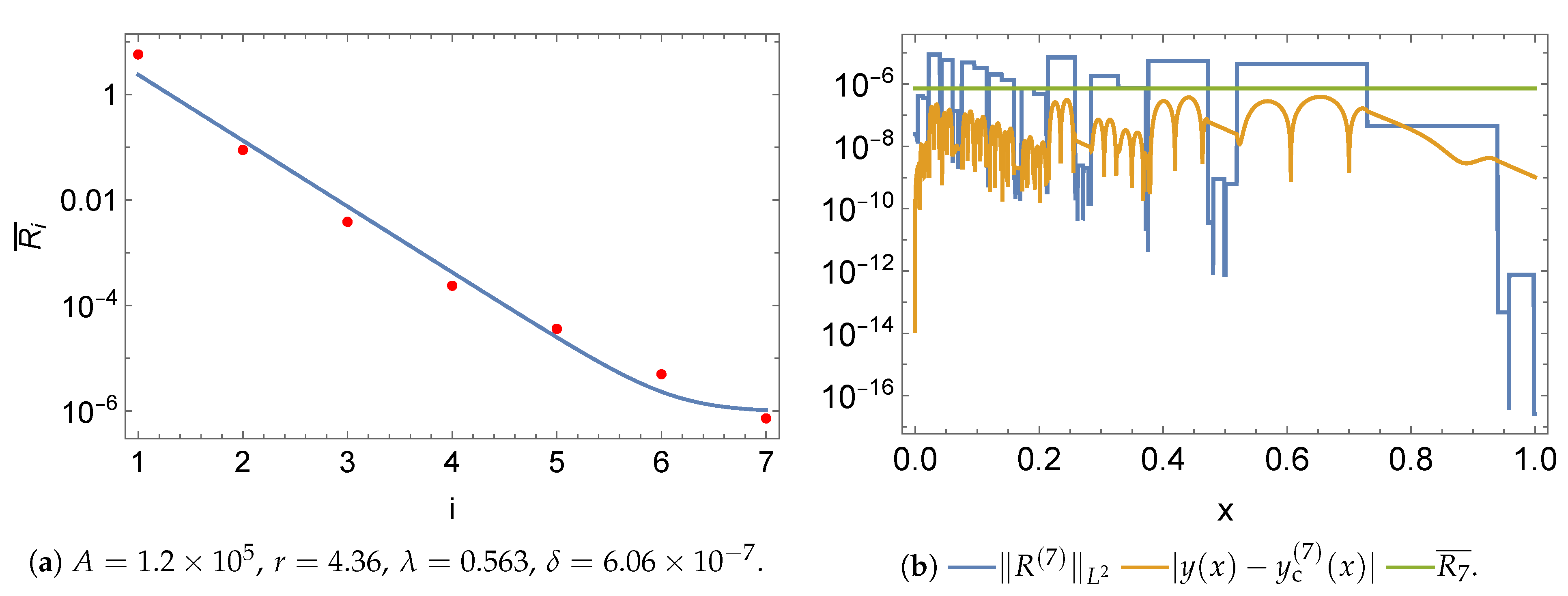
We perform the least-squares fitting of the logarithm of the set R to the logarithm of the upper bound (24). Figure 2a shows the least-squares fitted model (24) to the set R . The dots represent the set R and the solid line represents the least-squares fitted model (24). Figure 2b shows the residual, absolute local approximation error, and the mean value for the last iteration. The mean value R 7 ¯ is below the threshold value 10 6 . The L 2 norm of the approximation error y ( x ) y c ( 7 ) ( x ) 1.5 × 10 7 .
Example 2
(Hanging Bar Problem). We apply the collocation method on the hanging bar problem (14) and y ( x ) = e x ( x 1 ) 2 [61]. The approximate solution y c ( x ) is computed as discussed in Section 3.1.
We set the number of Sinc points to be inserted in all partitions as m = 2 N + 1 = 7 . The stopping criterion ε stop = 10 6 was used. The algorithm terminates after κ = 3 iterations and the number of points | S | = 350 .
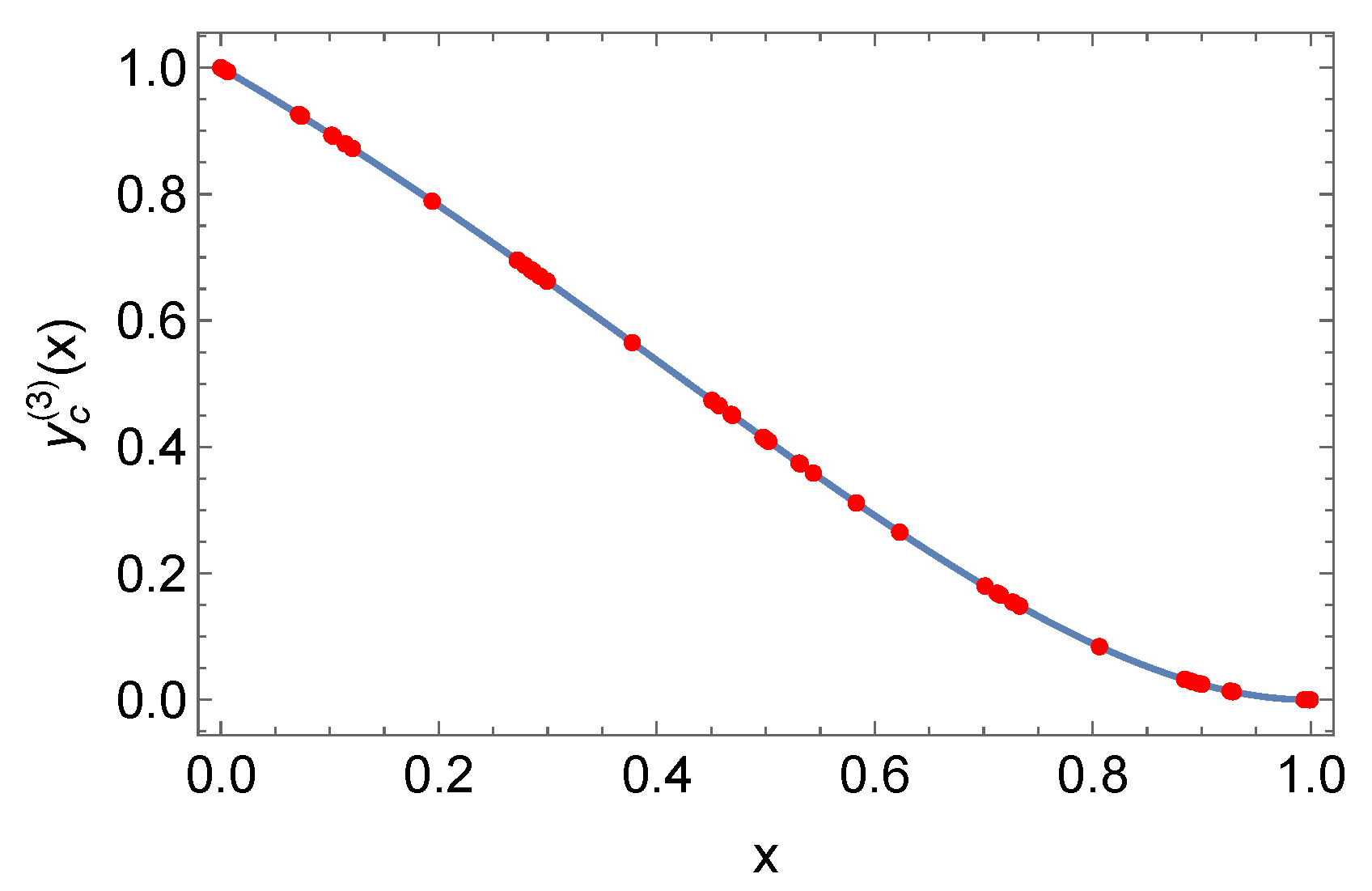
Figure 3 shows the approximate solution y c ( 3 ) ( x ) . A proper subset of the set of points S is shown as red dots, which are projected onto the approximate solution y c ( 3 ) ( x ) .
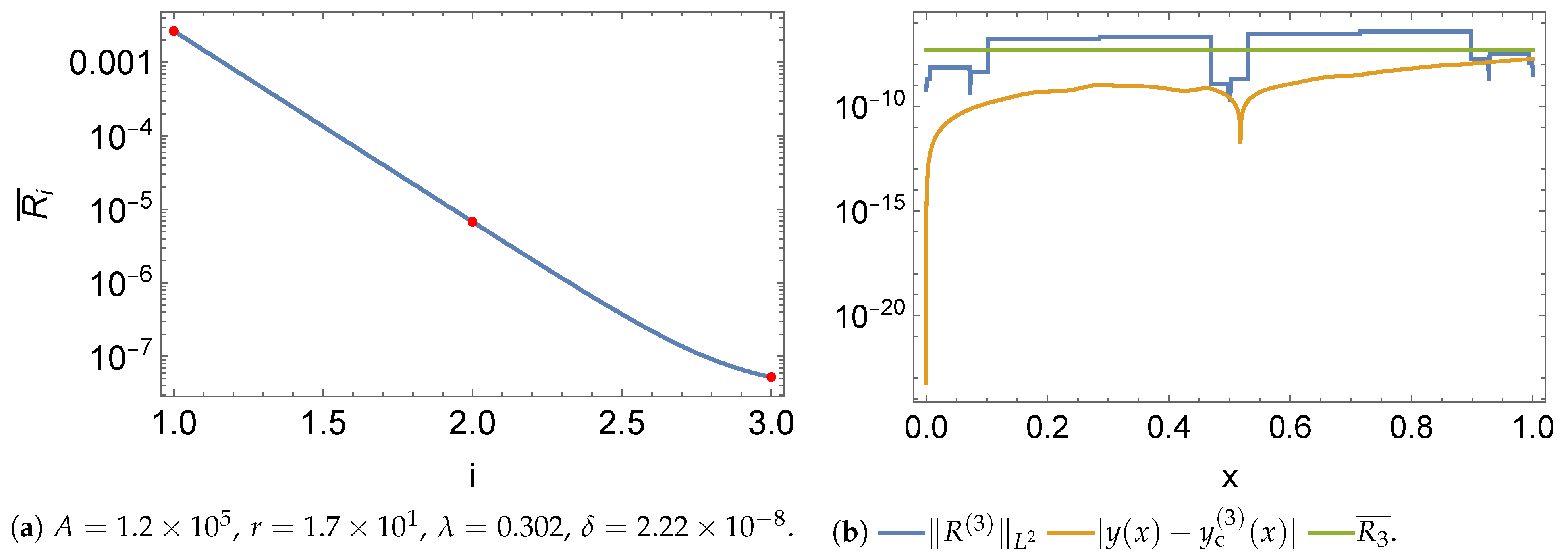
We perform the least-squares fitting of the logarithm of the set R to the logarithm of the upper bound (24). Figure 4a shows the least-squares fitted model (24) to the set R . Figure 4b shows the residual, absolute local approximation error, and the mean value for the last iteration. The mean value R 3 ¯ is below the threshold value 10 6 . The L 2 norm of the approximation error y ( x ) y c ( 3 ) ( x ) 5.82 × 10 9 .

5.3. Boundary Value Problem

We discuss a number of stiff BVPs [8] based on the general linear second-order BVP
( a ( x ) y ) + b ( x ) y + c ( x ) y = f ( x ) , x [ 0 , 1 ] ,
where a ( x ) > 0 , b ( x ) , c ( x ) are the coefficients, and f ( x ) is the source term.
Example 3.
We study the BVP (25) with a ( x ) = x + 0.01 , b ( x ) = c ( x ) = 0 , and f ( x ) = 1 . The exact solution is
y ( x ) = c 1 ln ( 1 + 100 x ) + c 2 x ,
where c 1 = 1 / ln ( 101 ) and c 2 = 0 are obtained from the boundary conditions y ( 0 ) = y ( 1 ) = 0 . The exact solution experiences a boundary layer near x = 0 .
We set the number of Sinc points to be inserted in all partitions as m = 2 N + 1 = 5 . The stopping criterion ε stop = 10 6 was used. The algorithm terminates after κ = 10 iterations and the number of points | S | = 2055 .
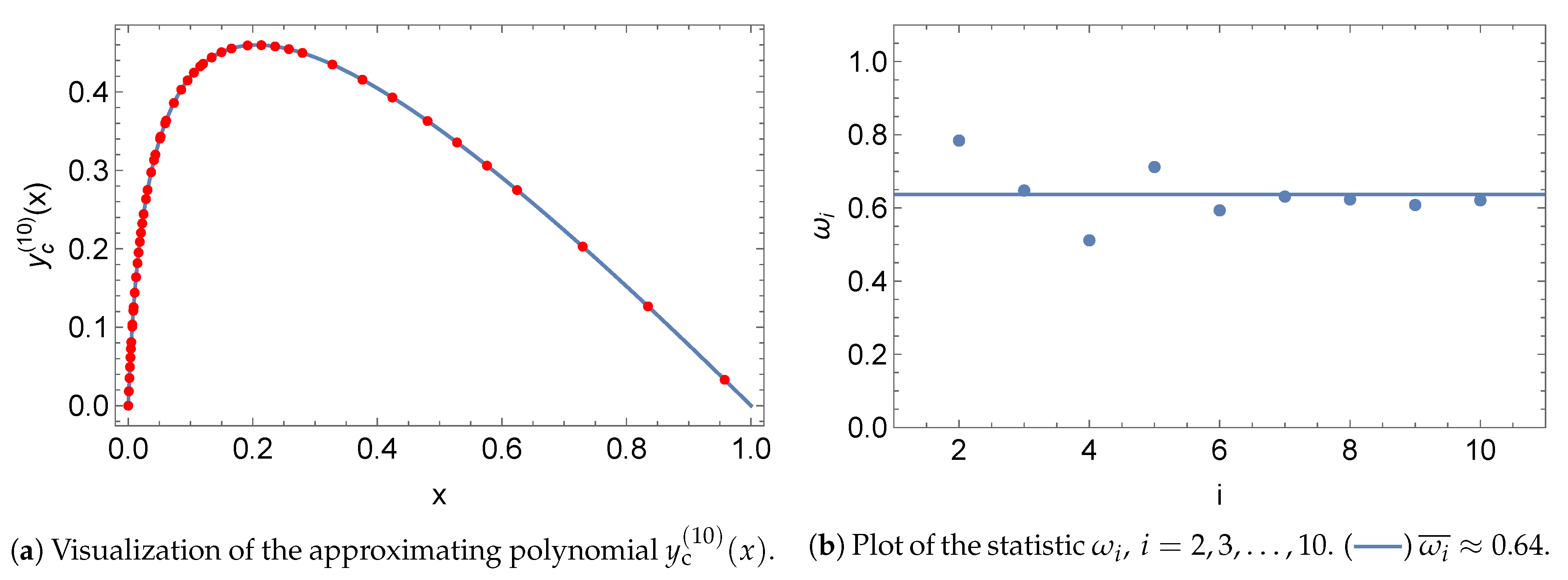
Figure 5a shows the approximate solution y c ( 10 ) ( x ) . A proper subset of the set of points S is shown as red dots, which are projected onto the approximate solution y c ( 10 ) ( x ) . We plot the statistic ω i as a function of the iteration index i , i = 2 , 3 , , 10 , in Figure 5b. It is observed that the oscillations are decaying and the statistic ω i is converging to an asymptotic value. The mean value ω i ¯ 0.64 .
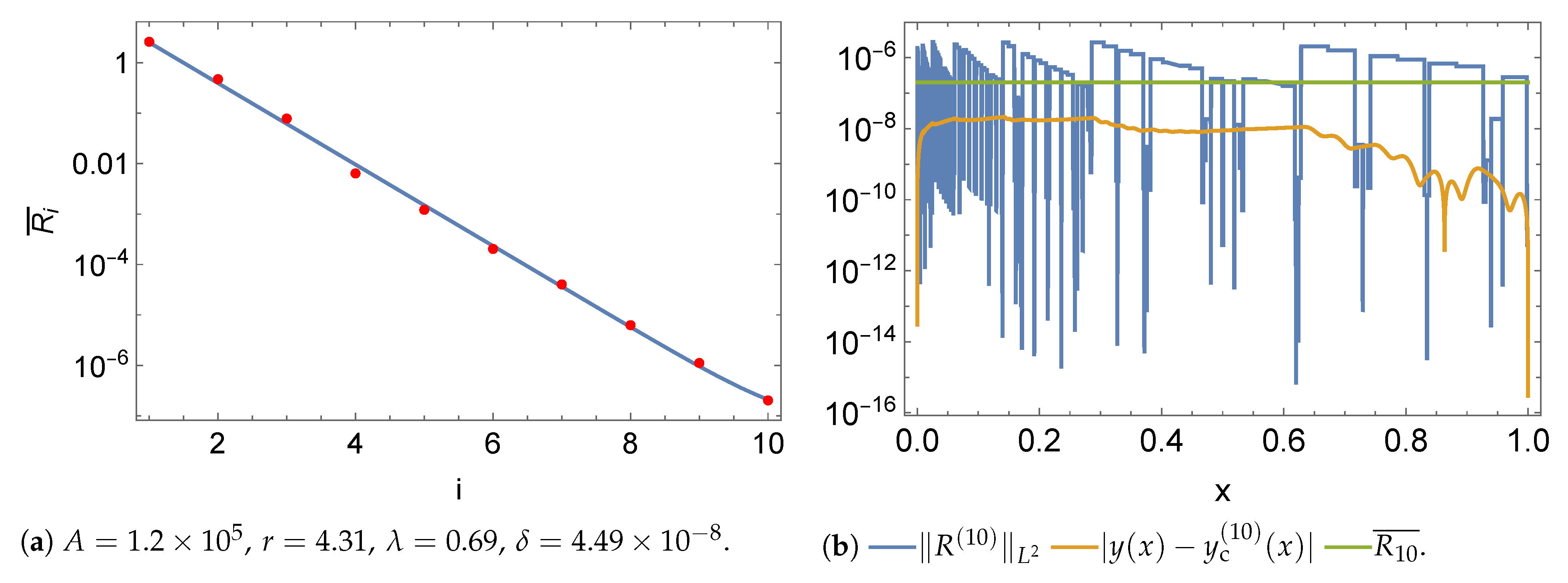
We perform the least-squares fitting of the logarithm of the set R to the logarithm of the upper bound (24). Figure 6a shows the least-squares fitted model (24) to the set R . Figure 6b shows the residual, absolute local approximation error, and the mean value for the last iteration. The plot of the L 2 norm values of the residual over the partitions demonstrates that fine partitions are formed near x = 0 due to the presence of the boundary layer. The mean value R 10 ¯ is below the threshold value 10 6 . The L 2 norm of the approximation error y ( x ) y c ( 10 ) ( x ) 1.12 × 10 8 . The threshold value in [8] is 0.05 .
Example 4.
We study the BVP (25) with a ( x ) = 0.01 , b ( x ) = 0 , c ( x ) = 1 , and f ( x ) = 1 / x . Using the variation of parameters method [62], the exact solution of this problem is
y ( x ) = 5 Ei ( 10 x ) exp ( 10 x ) + 5 Ei ( 10 x ) exp ( 10 x ) + c 1 exp ( 10 x ) + c 2 exp ( 10 x ) ,
where Ei ( x ) = x exp ( t ) t t is the exponential integral function [55] and
c 1 = c 2 = 5 Ei ( 10 ) exp ( 10 ) + 5 Ei ( 10 ) exp ( 10 ) exp ( 10 ) exp ( 10 ) .
The exact solution y ( x ) experiences a boundary layer near x = 0 and a slope change at approximately x = 0.5 . Equation (25) is multiplied by the factor x so that the residual R ( x ) does not contain a singularity at x = 0 .
We set the number of Sinc points to be inserted in all partitions as m = 2 N + 1 = 5 . The stopping criterion ε stop = 10 6 was used. The algorithm terminates after κ = 9 iterations and the number of points | S | = 1630 .
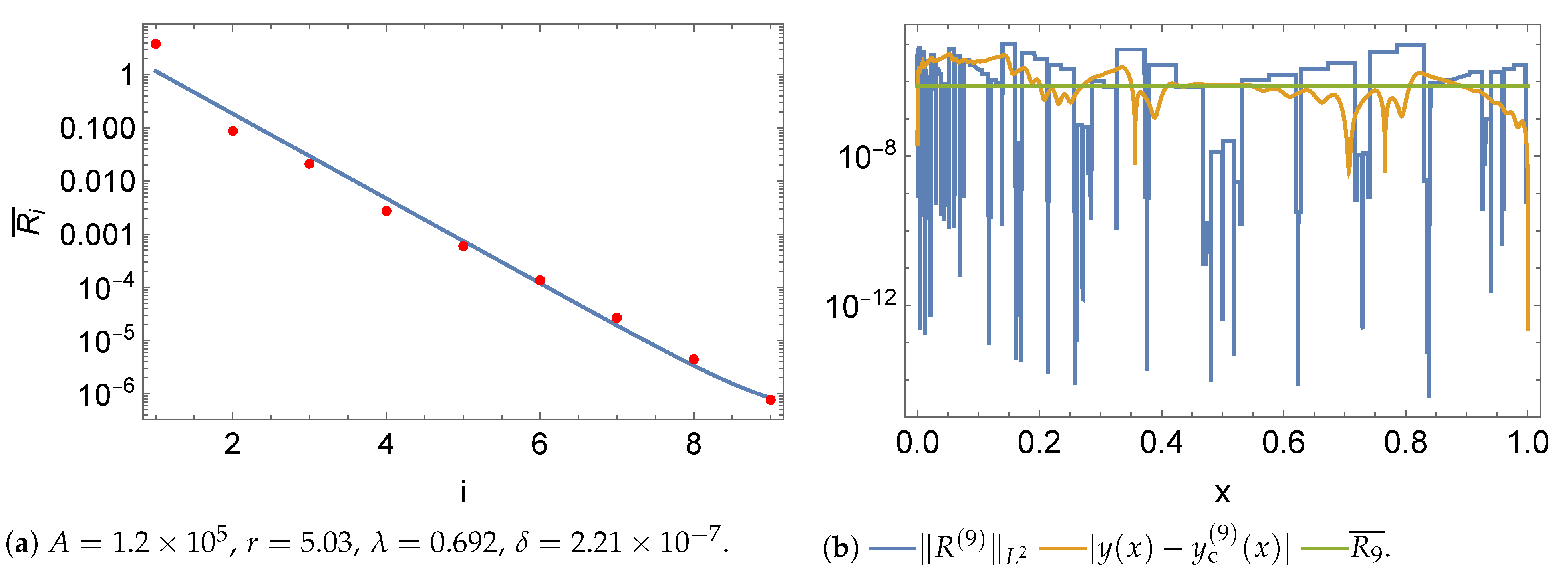
We perform the least-squares fitting of the logarithm of the set R to the logarithm of the upper bound (24). Figure 7a shows the least-squares fitted model (24) to the set R . Figure 7b shows the residual, absolute local approximation error, and the mean value for the last iteration. The plot of the L 2 norm values of the residual over the partitions shows that fine partitions are formed near x = 0 due to the presence of the boundary layer. The mean value R 9 ¯ is below the threshold value 10 6 . The L 2 norm of the approximation error y ( x ) y c ( 9 ) ( x ) 1.6 × 10 6 . The threshold value in [8] is 0.01 .
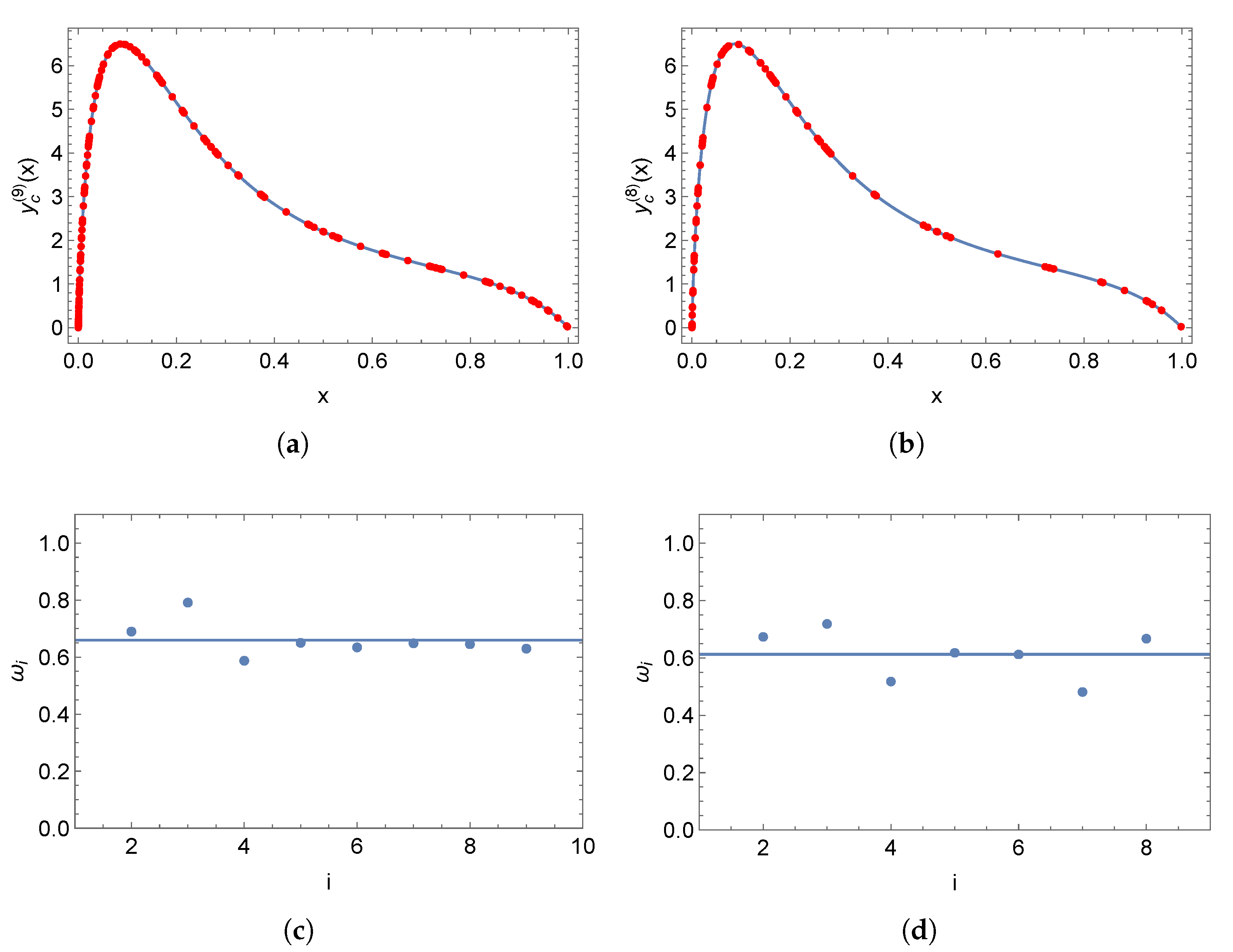
The approximating polynomial y c ( 9 ) ( x ) and a proper subset of the set of points S are shown in Figure 8a. The corresponding plot for the statistic ω i a is shown in Figure 8c. The oscillations are decaying and the mean value ω i ¯ 0.66 . It was mentioned that Equation (25) was multiplied by the factor x so that the residual R ( x ) does not contain a singularity at x = 0 . We replace the residual R ( x ) with the quantity y ( x ) y c ( x ) in Algorithm 4 and the BVP (25) contains the term 1 / x . We set the number of Sinc points to be inserted in all partitions as m = 2 N + 1 = 5 . The stopping criterion ε stop = 10 6 was used. The algorithm terminates after κ = 8 iterations and the number of points | S | = 730 , which is smaller than the one obtained from multiplying the residual by x. This is expected since the exact solution y ( x ) is used. The approximating polynomial y c ( 8 ) ( x ) and a proper subset of the set of points S are shown in Figure 8b. The corresponding plot for the statistic ω i is shown in Figure 8d. The mean value ω i ¯ 0.61 . It is observed that the statistic ω i oscillates around the mean ω i ¯ 0.61 .
Example 5.
We study a variation of Example 4, in which the source term f ( x ) = 1 x . Even though the source term has a singularity at x = 0 , its definite integral over the domain [ 0 , 1 ] is finite. The exact solution [62] is
y ( x ) = c 1 exp ( 10 x ) + c 2 exp ( 10 x ) + exp ( 10 x ) 5 π 10 erf 10 x exp ( 10 x ) 5 π 10 erfi 10 x ,
where
c 1 = c 2 = 5 π 2 e 20 erf 10 erfi 10 e 20 1 ,
erf ( x ) = 2 π 0 x e t 2 t ([55] § 7.1.1) is the error function, erfi ( x ) ı ( ı x ) = 2 π 0 x e t 2 t [63], and ı 2 = 1 . The solution y ( x ) has a boundary layer near x = 0 . Equation (25) is multiplied by the factor x so that the residual R ( x ) does not contain a singularity at x = 0 .
We set the number of Sinc points to be inserted in all partitions as m = 2 N + 1 = 5 . The stopping criterion ε stop = 10 6 was used. The algorithm terminates after κ = 7 iterations and the number of points | S | = 1183 .
We performed least-squares fitting of the logarithm of the set R to the logarithm of the upper bound (24). Figure 9a shows the least-squares fitted model (24) to the set R . Figure 9b shows the residual, absolute local approximation error, and the mean value for the last iteration. Fine partitions are formed near x = 0 due to the presence of the boundary layer, as seen in the plot of the L 2 norm values of the residual over the partitions. The mean value R 7 ¯ is below the threshold value 10 6 . The L 2 norm of the approximation error y ( x ) y c ( 7 ) ( x ) 2.18 × 10 7 .
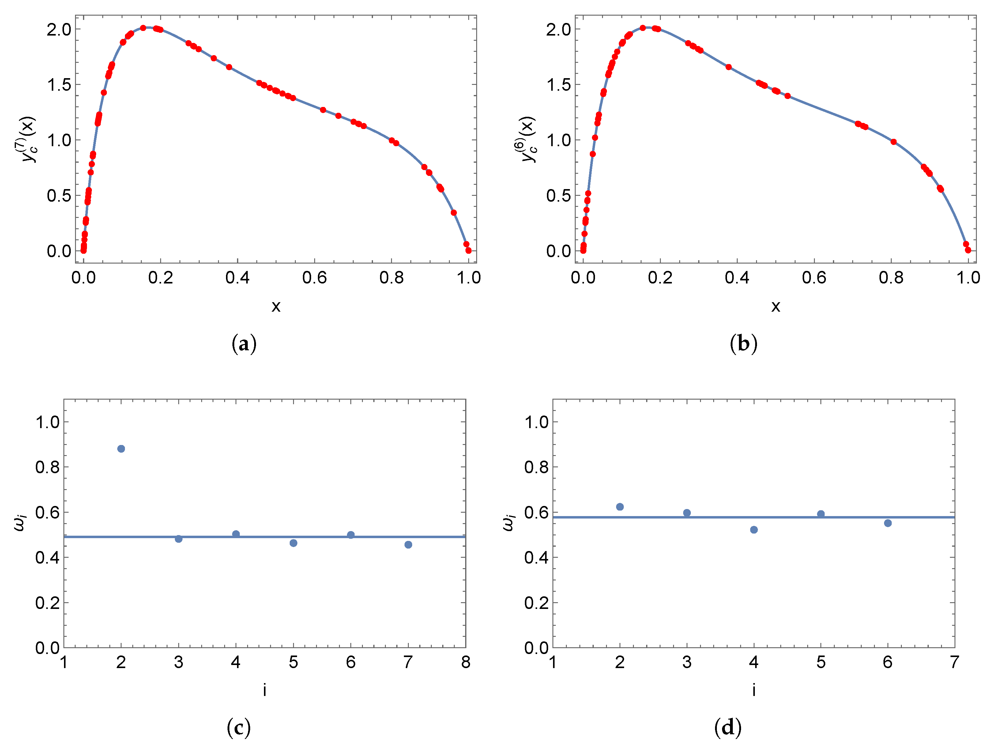
The approximating polynomial y c ( 7 ) ( x ) and a proper subset of the set of points S are shown in Figure 10a. The corresponding plot for the statistic ω i a is shown in Figure 10c. The statistic ω i oscillates around the median value ω ˜ i 0.49 . It was mentioned that Equation (25) was multiplied by the factor x so that the residual R ( x ) does not contain a singularity at x = 0 . We replace the residual R ( x ) with the quantity y ( x ) y c ( x ) in Algorithm 4 and the BVP (25) contains the term 1 / x . We set the number of Sinc points to be inserted in all partitions as m = 2 N + 1 = 5 . The stopping criterion ε stop = 10 6 was used. The algorithm terminates after κ = 6 iterations and the number of points | S | = 595 , which is smaller than the one obtained by multiplying the residual by x . This is expected since the exact solution y ( x ) is used. The approximating polynomial y c ( 6 ) ( x ) and a proper subset of the set of points S are shown in Figure 10b. The corresponding plot for the statistic ω i is shown in Figure 10d. The oscillations are decaying and the statistic ω i is converging to an asymptotic value. The mean value ω i ¯ is 0.58 .
Example 6.
We study a variation of Example 4, in which the source term f ( x ) = exp ( x ) 1 x . The source term has a removable singularity at x = 0 , since lim x 0 f ( x ) = 1 . The algorithm can directly solve the BVP, even though the residual contains the term exp ( x ) 1 x . The exact solution [62] is
y ( x ) = c 1 exp ( 10 x ) + c 2 exp ( 10 x ) 5 exp ( 10 x ) ( Ei ( 9 x ) Ei ( 10 x ) ) + 5 exp ( 10 x ) ( Ei ( 11 x ) Ei ( 10 x ) ) ,
where
c 1 = 5 e 20 Ei ( 10 ) e 20 Ei ( 9 ) Ei ( 10 ) + Ei ( 11 ) e 20 ln 10 9 e 20 ln 11 10 e 20 1
and
c 2 = 5 e 20 Ei ( 10 ) + e 20 Ei ( 9 ) + Ei ( 10 ) Ei ( 11 ) + ln 10 9 + ln 11 10 e 20 1 .
We set the number of Sinc points to be inserted in all partitions as m = 2 N + 1 = 5 . The stopping criterion ε stop = 10 6 was used. The algorithm terminates after κ = 8 iterations and the number of points | S | = 605 .
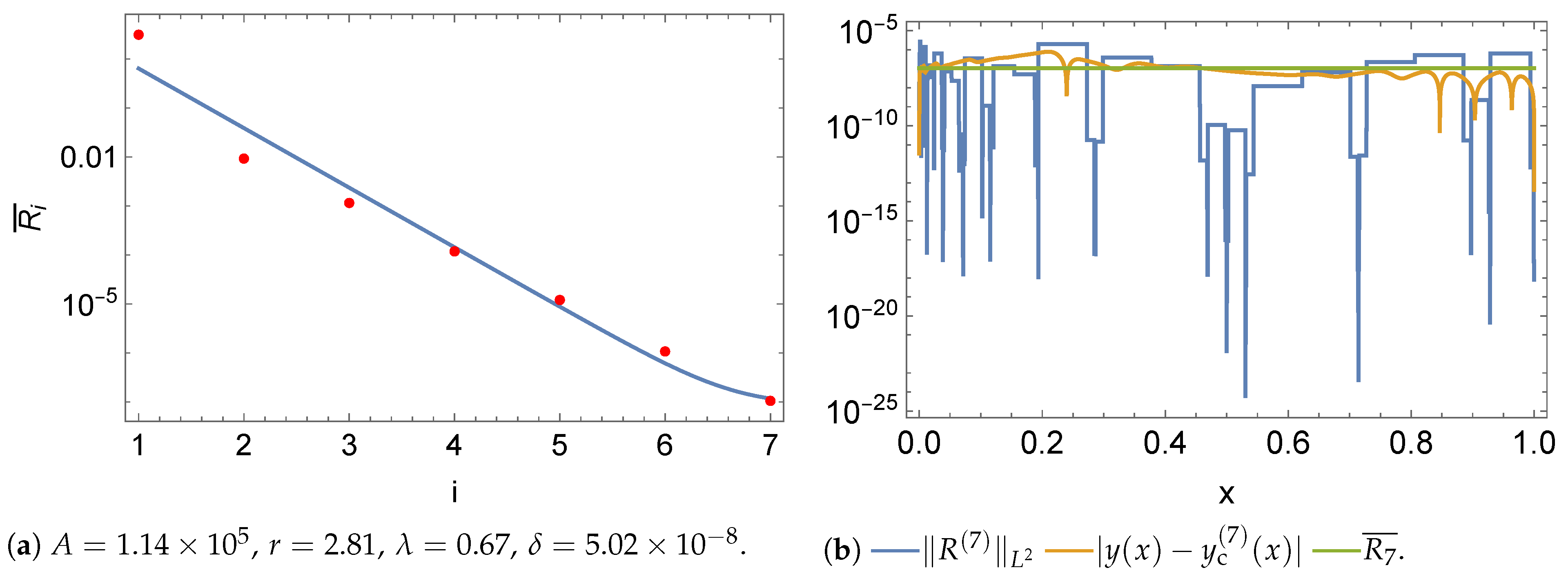
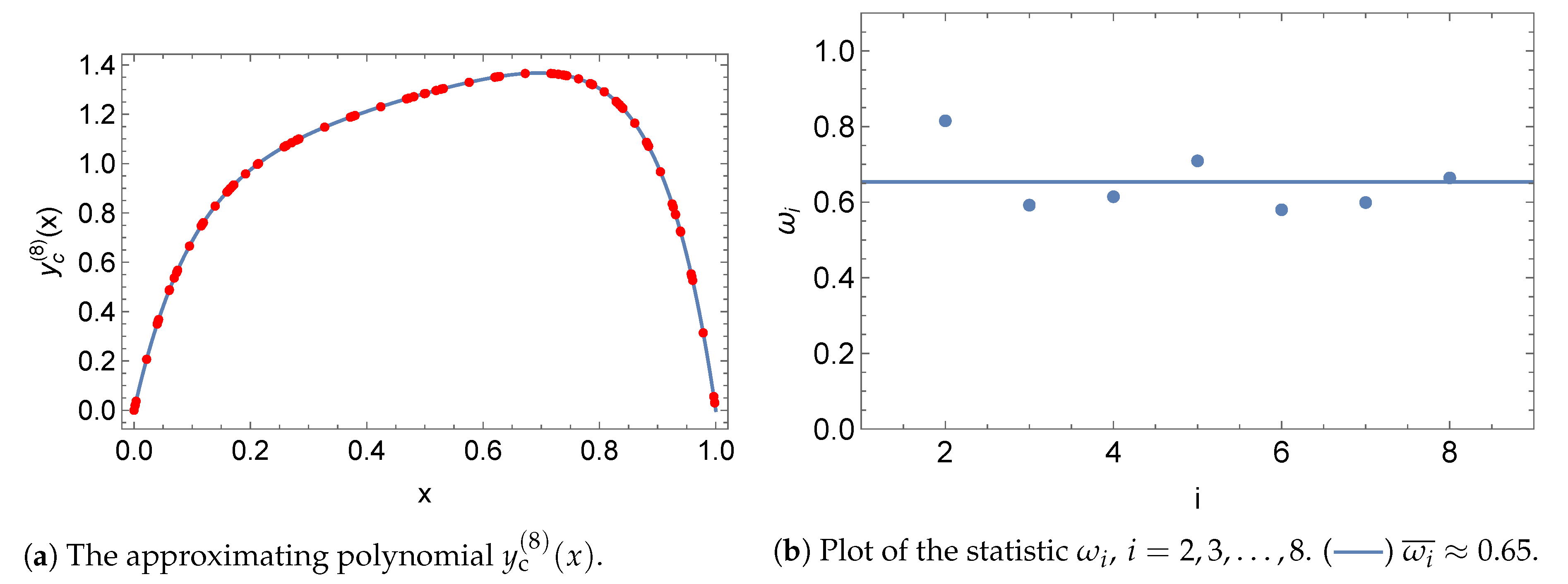
Figure 11a shows the approximate solution y c ( 8 ) ( x ) . A proper subset of the set of points S is shown as red dots, which are projected onto the approximate solution y c ( 8 ) ( x ) . We plot the statistic ω i as a function of the iteration index i , i = 2 , 3 , , 8 , in Figure 11b. The oscillations are decaying and the statistic ω i is converging to an asymptotic value. The mean value ω i ¯ 0.65 .
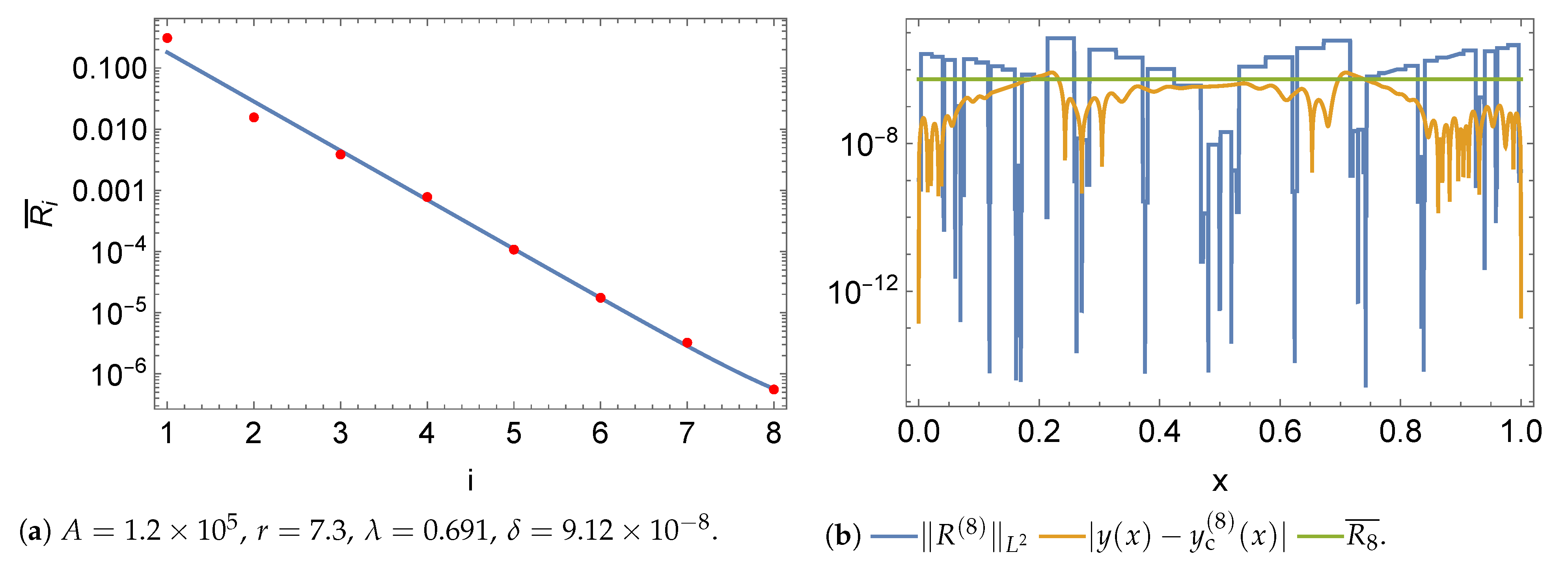
We perform the least-squares fitting of the logarithm of the set R to the logarithm of the upper bound (24). Figure 12a shows the least-squares fitted model (24) to the set R . Figure 12b shows the residual, absolute local approximation error, and the mean value for the last iteration. The mean value R 8 ¯ is below the threshold value 10 6 . The L 2 norm of the approximation error y ( x ) y c ( 10 ) ( x ) 3.1 × 10 7 .
Example 7.
We study the BVP (25) with a ( x ) = 0.02 , b ( x ) = 1 , c ( x ) = 0 , and f ( x ) = 1 . The exact solution is given by
y ( x ) = c 1 + c 2 exp ( 50 x ) + x ,
where c 1 = c 2 = 1 1 + exp ( 50 ) . The solution y ( x ) has a boundary layer near x = 1 .
We set the number of Sinc points to be inserted in all partitions as m = 2 N + 1 = 5 . The stopping criterion ε stop = 10 6 was used. The algorithm terminates after κ = 9 iterations and the number of points | S | = 1055 .
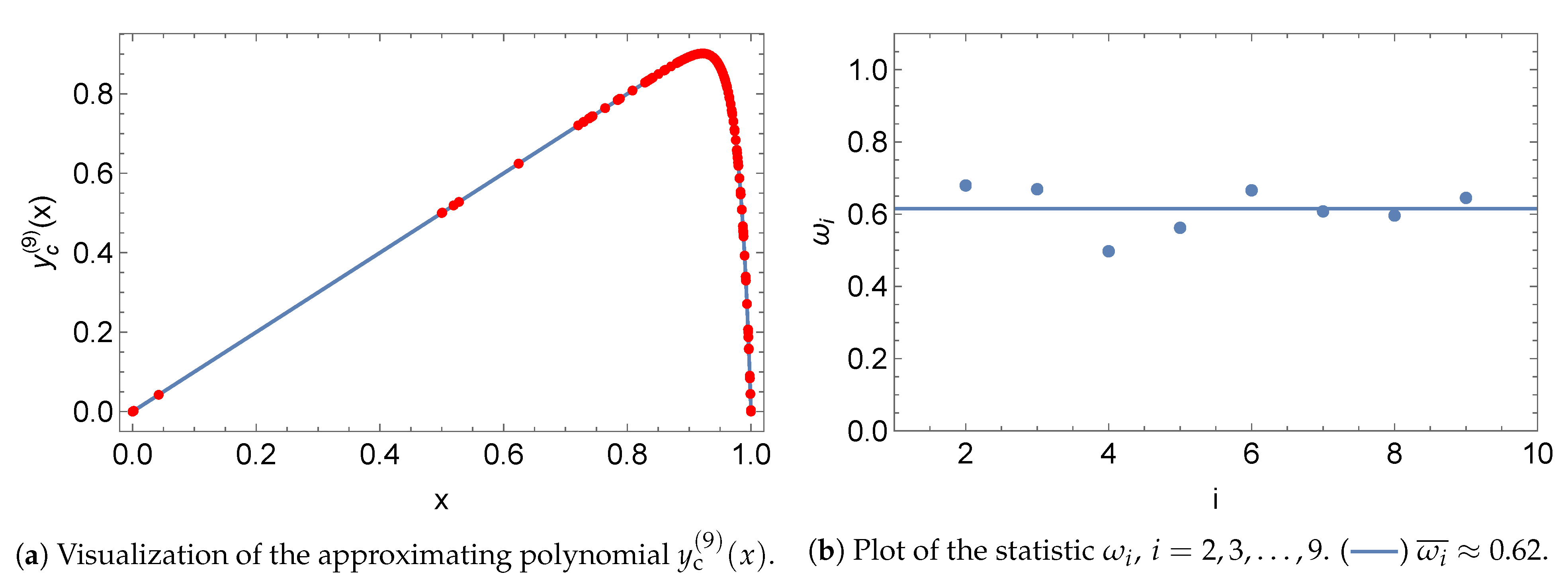
Figure 13a shows the approximate solution y c ( 9 ) ( x ) . A proper subset of the set of points S is shown as red dots, which are projected onto the approximate solution y c ( 9 ) ( x ) . We plot the statistic ω i as a function of the iteration index i , i = 2 , 3 , , 9 , in Figure 13b. The oscillations are decaying and the statistic ω i is converging to an asymptotic value. The mean value ω i ¯ is 0.62 .
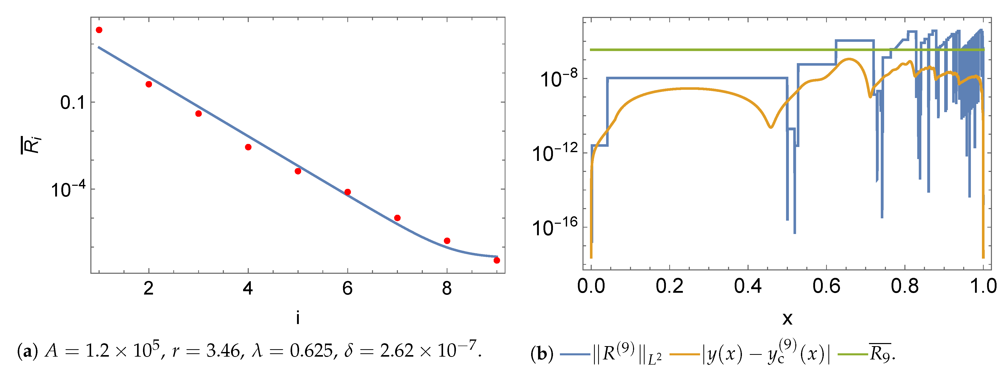
We perform the least-squares fitting of the logarithm of the set R to the logarithm of the upper bound (24). Figure 14a shows the least-squares fitted model (24) to the set R . Figure 14b shows the residual, absolute local approximation error, and the mean value for the last iteration. The plot of the L 2 norm values of the residual over the partitions shows that fine partitions are formed near x = 1 due to the presence of the boundary layer. One observation is that the mean value R 9 ¯ is below the threshold value 10 6 . The L 2 norm of the approximation error y ( x ) y c ( 9 ) ( x ) 2.36 × 10 8 and the threshold value in [8] is 0.02 .
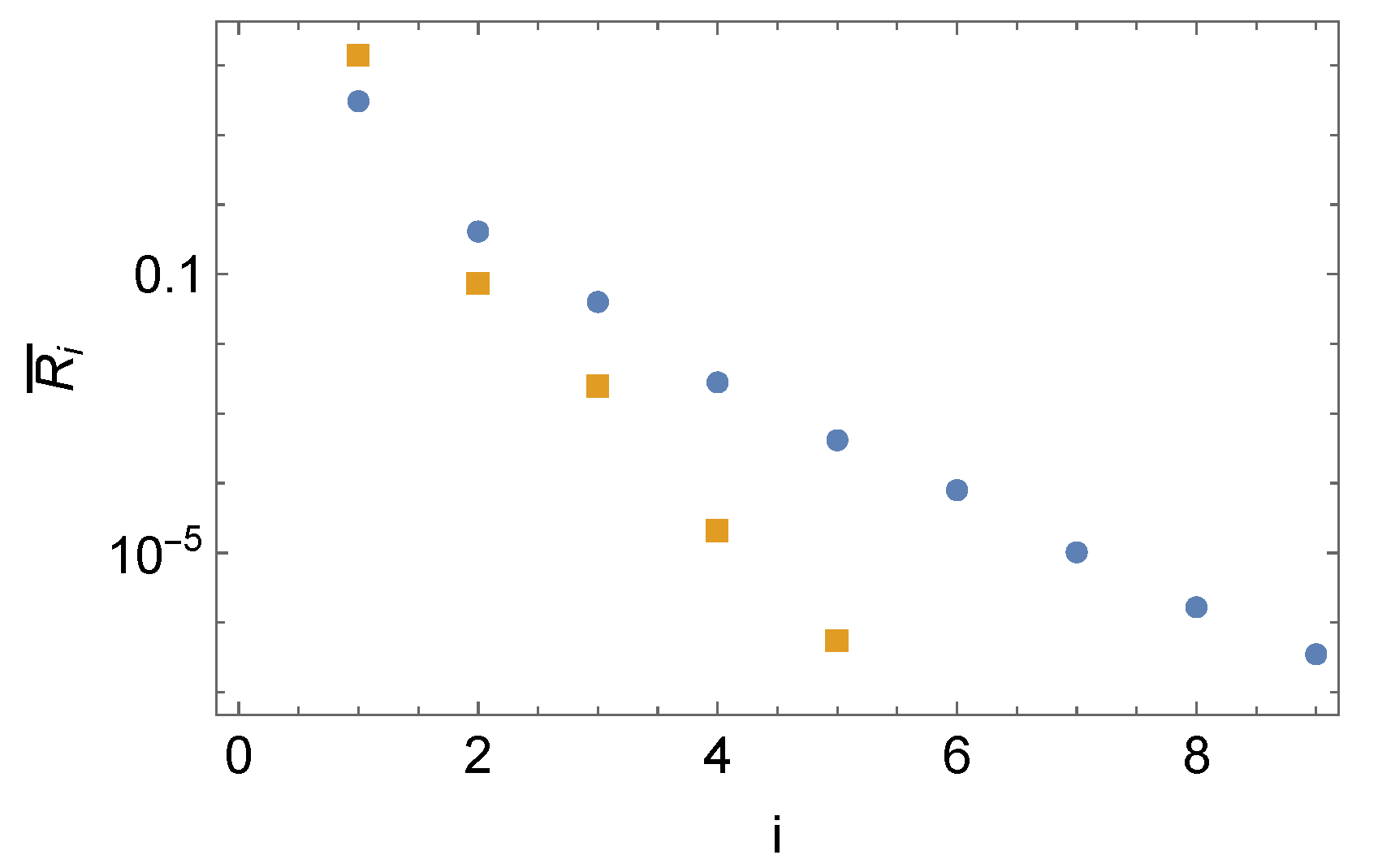
In this example, we increase the number of points per partition to m = 2 N + 1 = 7 to examine the effect of the increase on the convergence of the algorithm. The algorithm terminates after κ = 5 iterations and the number of points | S | = 350 . Figure 15 shows the set R for m = 2 N + 1 = 5 Sinc points and m = 2 N + 1 = 7 Sinc points. It is observed that increasing the number of Sinc points per partition leads to faster convergence and a fewer number of iterations.
Example 8.
We study the following BVP [28,64,65]
( υ ( x ) y ) = 2 1 + α ( x x ¯ ) ( arctan ( α ( x x ¯ ) ) + arctan ( α x ¯ ) )
with boundary conditions y ( 0 ) = y ( 1 ) = 0 , where α > 0 and
υ ( x ) = 1 α + α ( x x ¯ ) 2 .
For large values of α, the BVP (26) has an interior layer close to x ¯ [28]. The exact solution is given by
y ( x ) = ( 1 x ) arctan ( α ( x x ¯ ) ) + arctan ( α x ¯ ) .
We use the values reported in [64], i.e., α = 100 and x ¯ = 0.36388 . This value of x ¯ was chosen so that lim α y ( x ¯ + ) 2 [64].
We set the number of Sinc points to be inserted in all partitions as m = 2 N + 1 = 7 . The stopping criterion ε stop = 10 12 was used. The algorithm terminates after κ = 15 iterations and the number of points | S | = 21,469.
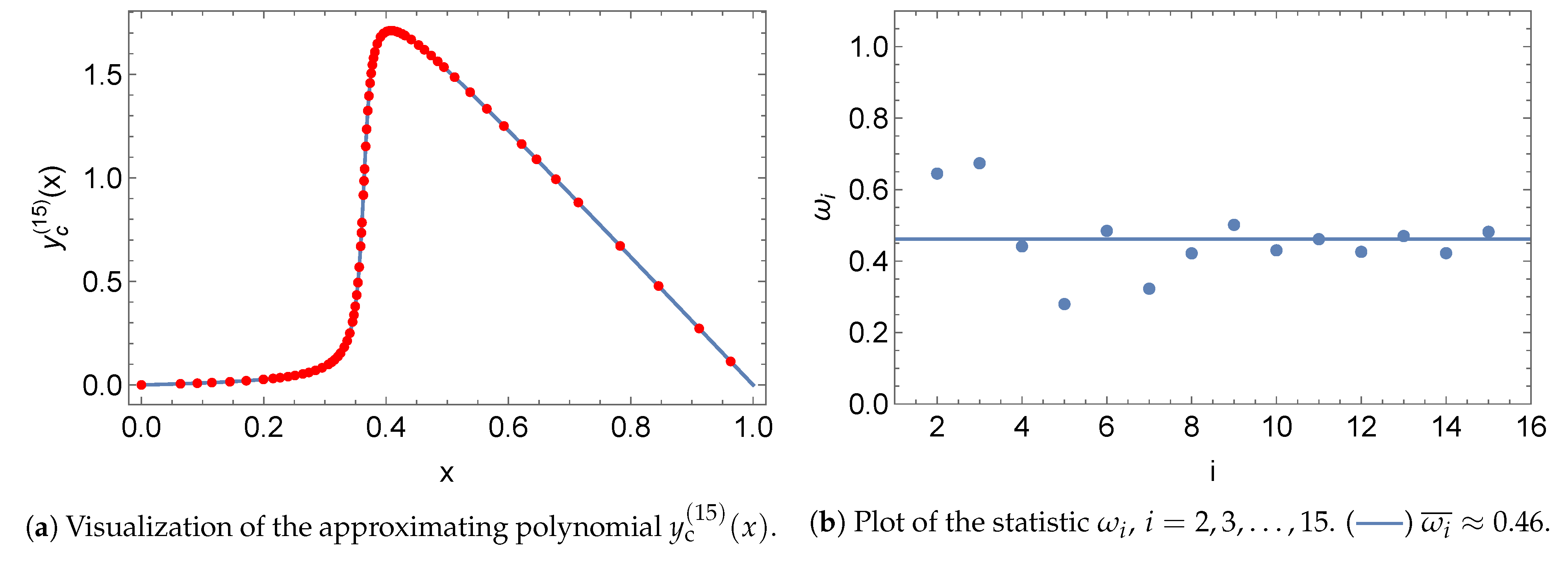
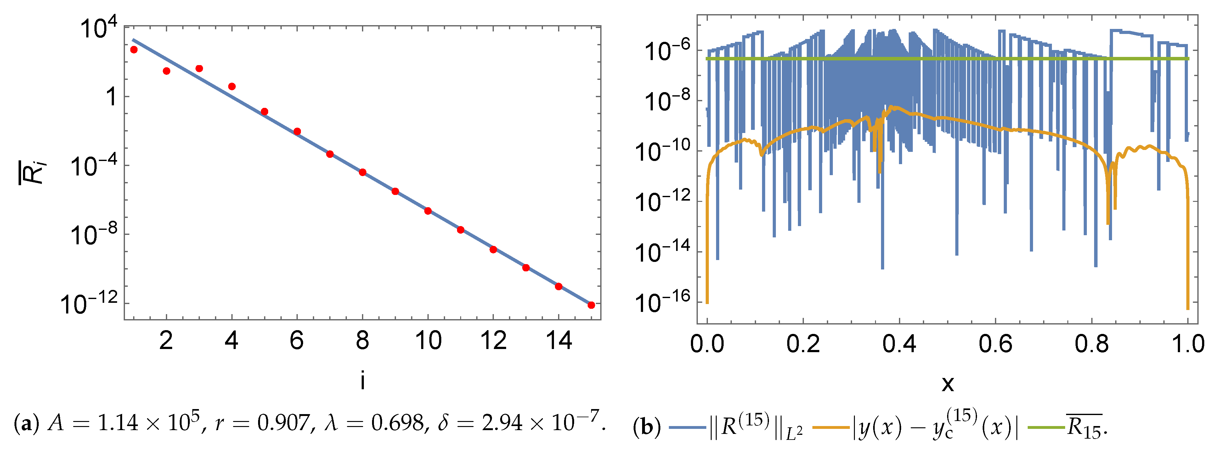
Figure 16a shows the approximate solution y c ( 15 ) ( x ) . A proper subset of the set of points S is shown as red dots, which are projected onto the approximate solution y c ( 15 ) ( x ) . We plot the statistic ω i as a function of the iteration index i , i = 2 , 3 , , 15 , in Figure 16b. One finding is that the oscillations are decaying and the statistic ω i is converging to an asymptotic value. The mean value ω i ¯ is 0.46 .
We perform the least-squares fitting of the logarithm of the set R to the logarithm of the upper bound (24), where the parameter δ is multiplied by 10 12 and 10 12 δ = O ( 10 19 ) . Figure 17a shows the least-squares fitted model (24) to the set R . The residual, absolute local approximation error, and the mean value for the last iteration are shown in Figure 17b. Fine partitions are formed near x = x ¯ due to the presence of the interior layer, as shown in the plot of the L 2 norm values of the residual over the partitions. The mean value R 13 ¯ is below the threshold ε stop = 10 12 .
We compare the L 2 norm of the approximation error of our adaptive piecewise Poly-Sinc method with other methods in Table 1. Method [28] requires a parameter for the construction of refinement intervals. The L 2 norm value of the approximation error is smaller than those reported in [28,65].
Example 9.
We consider the BVP [66,67]
ϵ y x y = ϵ π 2 cos ( π x ) + π x sin ( π x ) , x [ 1 , 1 ] ,
with boundary conditions y ( 1 ) = 2 , y ( 1 ) = 0 and ϵ > 0 is a parameter. The exact solution follows as
y ( x ) = cos ( π x ) + ( x / 2 ϵ ) ( 1 / 2 ϵ ) .
The exact solution has a shock layer near x = 0 [66]. We set ϵ = 10 6 [67].
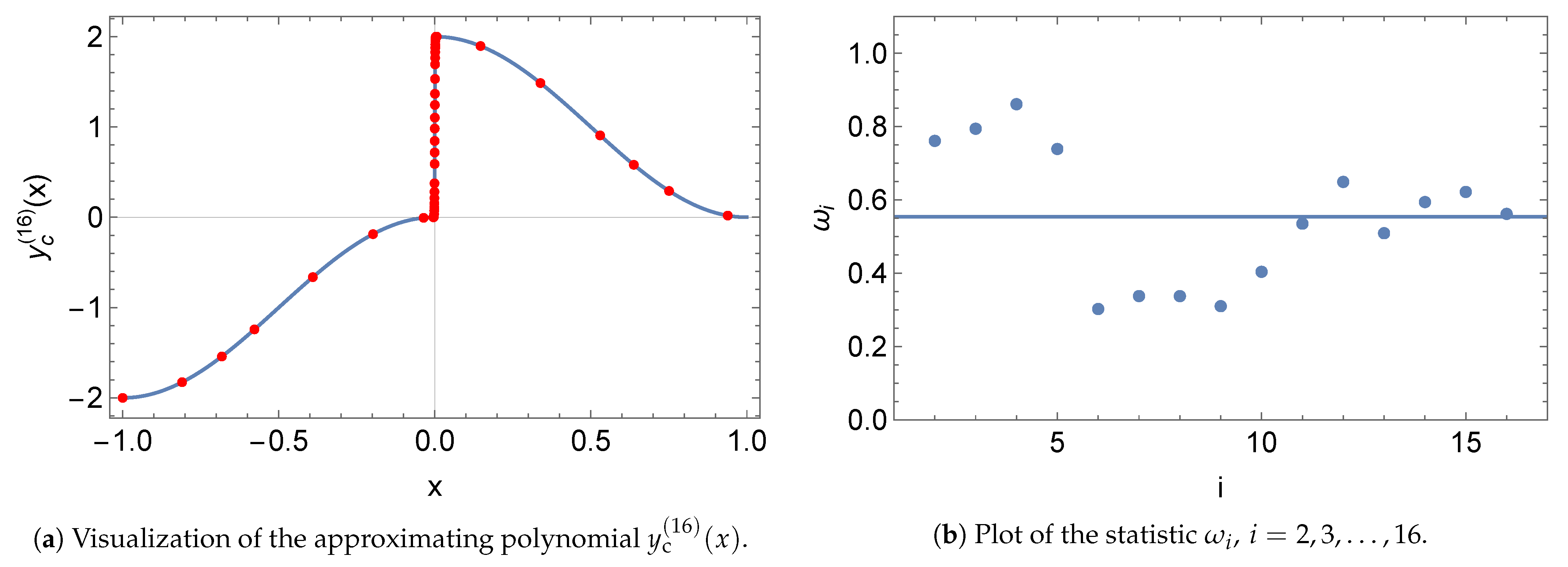
We set the number of Sinc points to be inserted in all partitions as m = 2 N + 1 = 5 . The stopping criterion ε stop = 10 11 was used. The algorithm terminates after κ = 16 iterations and the number of points | S | = 18530 .
Figure 18a shows the approximate solution y c ( 16 ) ( x ) . A proper subset of the set of points S is shown as red dots, which are projected onto the approximate solution y c ( 16 ) ( x ) . We plot the statistic ω i as a function of the iteration index i , i = 2 , 3 , , 16 , in Figure 18b. The oscillations are decaying and the statistic ω i is converging to an asymptotic value. The mean value ω i ¯ 0.55 .
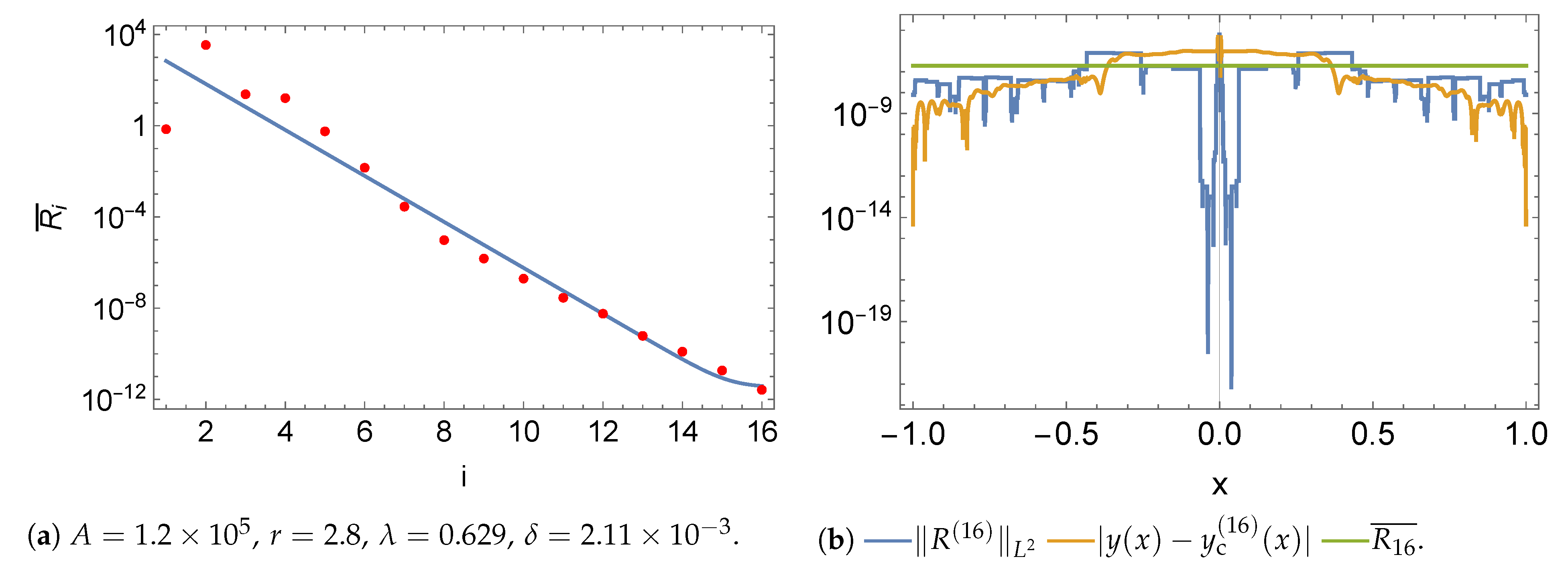
We perform the least-squares fitting of the logarithm of the set R to the logarithm of the upper bound (24), where the parameter δ is multiplied by the factor 10 9 and 10 9 δ = O ( 10 12 ) . Figure 19a shows the least-squares fitted model (24) to the set R . The residual, absolute local approximation error, and the mean value for the last iteration are shown in Figure 19b. The plot of the L 2 norm values of the residual over the partitions show that fine partitions are formed near x = 0 due to the presence of the shock layer. The mean value R 16 ¯ is below the threshold ε stop = 10 11 .
We compare the supremum norm of the approximation error of our adaptive piecewise Poly-Sinc method with other methods in Table 2. B —splines were used as basis functions [67]. The supremum norm result is in the same order as that of [67]. Our adaptive method can reach a smaller value if we set ε stop < 10 11 .
We observe that the processing times differ among the many problems we look at. This is due to two factors: first, the fact that we are aiming for a very exact outcome; and second, the fact that there are many sorts of challenges. Therefore, listing the computing time in seconds is meaningless since it would only indicate the computational power used on our machine, which will vary for various users. Overall, it is evident that using adaptive techniques takes longer than using a simple collocation approach or finite element methods with a lower accuracy. In our examples, we used a stopping criterion of 10 6 or less. As a result, our goal is to complete the computation in the most accurate way feasible rather than the quickest way possible. This will inevitably lengthen the processing time for some problems, such as stiff or layer problems.

6. Conclusions

In this paper, we developed an adaptive piecewise collocation method based on Poly-Sinc interpolation for the approximation of solutions to ODEs. We showed the exponential convergence in the number of iterations of the a priori error estimate obtained from the piecewise collocation method, and provided that a good estimate of the exact solution y ( x ) at the Sinc points exists. We used a statistical approach for partition refinement, in which we computed the fraction of a standard deviation as the ratio of the mean absolute deviation to the sample standard deviation. We demonstrated by several examples that an exponential error decay is observed for regular ODEs and ODEs whose exact solutions exhibit an interior layer, a boundary layer, and a shock layer. We showed that our adaptive algorithm can deliver results with high accuracy at the expense of the slower computation for stiff ODEs.

Author Contributions

Conceptualization, M.Y. and G.B.; methodology, O.K., M.Y. and G.B.; software, O.K. and G.B.; validation, O.K., H.E.-S., M.Y. and G.B.; formal analysis, O.K. and H.E.-S.; investigation, H.E.-S. and G.B.; resources, not applicable; data curation, not applicable; writing—original draft preparation, O.K.; writing—review and editing, G.B. and O.K.; visualization, O.K.; supervision, H.E.-S., M.Y. and G.B.; project administration, H.E.-S.; funding acquisition, there is no funding of this article. All authors have read and agreed to the published version of the manuscript.

Funding

M.Y. is funded by BMBF under the contract 05M20VSA.

Institutional Review Board Statement

Not applicable.

Informed Consent Statement

Not applicable.

Data Availability Statement

Not applicable.

Acknowledgments

The authors thank Frank Stenger for his insightful conversations and continuous guidance.

Conflicts of Interest

The authors declare no conflict of interest.

References

  1. Hairer, E.; Nørsett, S.P.; Wanner, G. Solving Ordinary Differential Equations I: Nonstiff Problems; Springer: Berlin/Heidelberg, Germany, 1993. [Google Scholar]
  2. Hairer, E.; Wanner, G. Solving Ordinary Differential Equations II: Stiff and Differential-Algebraic Problems; Springer: Berlin/Heidelberg, Germany, 1996. [Google Scholar]
  3. Hairer, E.; Wanner, G.; Lubich, C. Geometric Numerical Integration: Structure-Preserving Algorithms for Ordinary Differential Equations; Springer: Berlin/Heidelberg, Germany, 2006. [Google Scholar]
  4. Ascher, U.M.; Mattheij, R.M.M.; Russell, R.D. Numerical Solution of Boundary Value Problems for Ordinary Differential Equations; SIAM: Philadelphia, PA, USA, 1995. [Google Scholar]
  5. Stakgold, I. Boundary Value Problems of Mathematical Physics: Volume I & II; SIAM: Philadelphia, PA, USA, 2000. [Google Scholar]
  6. Axelsson, O.; Barker, V.A. Finite Element Solution of Boundary Value Problems: Theory and Computation; SIAM: Philadelphia, PA, USA, 2001. [Google Scholar]
  7. Keller, H.B. Numerical Methods for Two-Point Boundary-Value Problems; Dover Publications, Inc.: Mineola, NY, USA, 2018. [Google Scholar]
  8. Eriksson, K.; Estep, D.; Hansbo, P.; Johnson, C. Introduction to adaptive methods for differential equations. Acta Numer. 1995, 4, 105–158. [Google Scholar] [CrossRef]
  9. Wright, K. Adaptive methods for piecewise polynomial collocation for ordinary differential equations. BIT Numer. Math. 2007, 47, 197–212. [Google Scholar] [CrossRef]
  10. Tao, Z.; Jiang, Y.; Cheng, Y. An adaptive high-order piecewise polynomial based sparse grid collocation method with applications. J. Comput. Phys. 2021, 433, 109770. [Google Scholar] [CrossRef]
  11. Logg, A. Multi-adaptive Galerkin methods for ODEs. I. SIAM J. Sci. Comput. 2003, 24, 1879–1902. [Google Scholar] [CrossRef]
  12. Logg, A. Multi-adaptive Galerkin methods for ODEs. II. Implementation and applications. SIAM J. Sci. Comput. 2004, 25, 1119–1141. [Google Scholar] [CrossRef]
  13. Baccouch, M. Analysis of a posteriori error estimates of the discontinuous Galerkin method for nonlinear ordinary differential equations. Appl. Numer. Math. 2016, 106, 129–153. [Google Scholar] [CrossRef]
  14. Baccouch, M. A posteriori error estimates and adaptivity for the discontinuous Galerkin solutions of nonlinear second-order initial-value problems. Appl. Numer. Math. 2017, 121, 18–37. [Google Scholar] [CrossRef]
  15. Cao, Y.; Petzold, L. A posteriori error estimation and global error control for ordinary differential equations by the adjoint method. SIAM J. Sci. Comput. 2004, 26, 359–374. [Google Scholar] [CrossRef]
  16. Kehlet, B.; Logg, A. A posteriori error analysis of round-off errors in the numerical solution of ordinary differential equations. Numer. Algorithms 2017, 76, 191–210. [Google Scholar] [CrossRef]
  17. Moon, K.S.; Szepessy, A.; Tempone, R.; Zouraris, G.E. A variational principle for adaptive approximation of ordinary differential equations. Numer. Math. 2003, 96, 131–152. [Google Scholar] [CrossRef]
  18. Moon, K.S.; Szepessy, A.; Tempone, R.; Zouraris, G.E. Convergence rates for adaptive approximation of ordinary differential equations. Numer. Math. 2003, 96, 99–129. [Google Scholar] [CrossRef]
  19. Moon, K.S.; von Schwerin, E.; Szepessy, A.; Tempone, R. An adaptive algorithm for ordinary, stochastic and partial differential equations. In Recent Advances in Adaptive Computation; American Mathematical Society: Providence, RI, USA, 2005; Volume 383, Contemporary Mathematics; pp. 325–343. [Google Scholar] [CrossRef]
  20. Johnson, C. Error estimates and adaptive time-step control for a class of one-step methods for stiff ordinary differential equations. SIAM J. Numer. Anal. 1988, 25, 908–926. [Google Scholar] [CrossRef]
  21. Estep, D.; French, D. Global error control for the continuous Galerkin finite element method for ordinary differential equations. RAIRO Modél. Math. Anal. Numér. 1994, 28, 815–852. [Google Scholar] [CrossRef]
  22. Estep, D.; Ginting, V.; Tavener, S. A posteriori analysis of a multirate numerical method for ordinary differential equations. Comput. Methods Appl. Mech. Eng. 2012, 223/224, 10–27. [Google Scholar] [CrossRef]
  23. Stenger, F. Polynomial function and derivative approximation of Sinc data. J. Complex. 2009, 25, 292–302. [Google Scholar] [CrossRef]
  24. Stenger, F.; Youssef, M.; Niebsch, J. Improved Approximation via Use of Transformations. In Multiscale Signal Analysis and Modeling; Shen, X., Zayed, A.I., Eds.; Springer: New York, NY, USA, 2013; pp. 25–49. [Google Scholar] [CrossRef]
  25. Khalil, O.A.; El-Sharkawy, H.A.; Youssef, M.; Baumann, G. Adaptive piecewise Poly-Sinc methods for function approximation. Submitted to Applied Numerical Mathematics. 2022. [Google Scholar]
  26. Carey, G.F.; Humphrey, D.L. Finite element mesh refinement algorithm using element residuals. In Codes for Boundary-Value Problems in Ordinary Differential Equations; Childs, B., Scott, M., Daniel, J.W., Denman, E., Nelson, P., Eds.; Springer: Berlin/Heidelberg, Germany, 1979; pp. 243–249. [Google Scholar] [CrossRef]
  27. Carey, G.F. Adaptive refinement and nonlinear fluid problems. Comput. Methods Appl. Mech. Eng. 1979, 17–18, 541–560. [Google Scholar] [CrossRef]
  28. Carey, G.F.; Humphrey, D.L. Mesh refinement and iterative solution methods for finite element computations. Int. J. Numer. Methods Eng. 1981, 17, 1717–1734. [Google Scholar] [CrossRef]
  29. Geary, R.C. The ratio of the mean deviation to the standard deviation as a test of normality. Biometrika 1935, 27, 310–332. [Google Scholar] [CrossRef]
  30. Stenger, F. Handbook of Sinc Numerical Methods; CRC Press: Boca Raton, FL, USA, 2011. [Google Scholar] [CrossRef]
  31. Youssef, M.; Pulch, R. Poly-Sinc solution of stochastic elliptic differential equations. J. Sci. Comput. 2021, 87, 1–19. [Google Scholar] [CrossRef]
  32. Stenger, F.; El-Sharkawy, H.A.M.; Baumann, G. The Lebesgue Constant for Sinc Approximations. In New Perspectives on Approximation and Sampling Theory: Festschrift in Honor of Paul Butzer’s 85th Birthday; Zayed, A.I., Schmeisser, G., Eds.; Springer International Publishing: Cham, Switzerland, 2014; pp. 319–335. [Google Scholar] [CrossRef]
  33. Youssef, M.; El-Sharkawy, H.A.; Baumann, G. Lebesgue constant using Sinc points. Adv. Numer. Anal. 2016, 2016. [Google Scholar] [CrossRef]
  34. Youssef, M.; Baumann, G. Collocation method to solve elliptic equations, bivariate Poly-Sinc approximation. J. Progress. Res. Math. 2016, 7, 1079–1091. [Google Scholar]
  35. Youssef, M. Poly-Sinc Approximation Methods. Ph.D. Thesis, German University in Cairo, New Cairo, Egypt, 2017. [Google Scholar]
  36. Youssef, M.; Baumann, G. Troesch’s problem solved by Sinc methods. Math. Comput. Simul. 2019, 162, 31–44. [Google Scholar] [CrossRef]
  37. Khalil, O.A.; Baumann, G. Discontinuous Galerkin methods using poly-sinc approximation. Math. Comput. Simul. 2021, 179, 96–110. [Google Scholar] [CrossRef]
  38. Khalil, O.A.; Baumann, G. Convergence rate estimation of poly-Sinc-based discontinuous Galerkin methods. Appl. Numer. Math. 2021, 165, 527–552. [Google Scholar] [CrossRef]
  39. Stoer, J.; Bulirsch, R. Introduction to Numerical Analysis; Springer: New York, NY, USA, 2002. [Google Scholar] [CrossRef]
  40. Baumann, G.; Stenger, F. Sinc-approximations of fractional operators: A computing approach. Mathematics 2015, 3, 444–480. [Google Scholar] [CrossRef] [Green Version]
  41. Coddington, E.A. An introduction to Ordinary Differential Equations; Dover Publications, Inc.: Mineola, NY, USA, 1989. [Google Scholar]
  42. Lund, J.; Bowers, K.L. Sinc Methods for Quadrature and Differential Equations; SIAM: Philadelphia, PA, USA, 1992; Volume 32. [Google Scholar]
  43. Stenger, F. Numerical Methods Based on Sinc and Analytic Functions; Springer Series in Computational Mathematics; Springer: New York, NY, USA, 1993; Volume 20. [Google Scholar] [CrossRef]
  44. Youssef, M.; Baumann, G. Solution of nonlinear singular boundary value problems using polynomial-Sinc approximation. Commun. Fac. Sci. Univ. Ank. Sér. A1 Math. Stat. 2014, 63, 41–58. [Google Scholar] [CrossRef]
  45. Baumann, G. (Ed.) New Sinc Methods of Numerical Analysis; Trends in Mathematics; Birkhäuser/Springer: Cham, Switzerland, 2021. [Google Scholar] [CrossRef]
  46. Vesely, F.J. Computational Physics: An Introduction; Kluwer Academic/Plenum Publishers: New York, NY, USA, 2001. [Google Scholar]
  47. Carey, G.; Finlayson, B.A. Orthogonal collocation on finite elements. Chem. Eng. Sci. 1975, 30, 587–596. [Google Scholar] [CrossRef]
  48. Strang, G. Computational Science and Engineering; Wellesley-Cambridge Press: Wellesley, MA, USA, 2007. [Google Scholar]
  49. Wazwaz, A.M. Linear and Nonlinear Integral Equations: Methods and Applications; Higher Education Press: Beijing, China; Springer: Berlin/Heidelberg, Germany, 2011. [Google Scholar] [CrossRef]
  50. Cormen, T.H.; Leiserson, C.E.; Rivest, R.L.; Stein, C. Introduction to Algorithms; MIT Press: Cambridge, MA, USA, 2009. [Google Scholar]
  51. Haasdonk, B.; Ohlberger, M. Reduced basis method for finite volume approximations of parametrized linear evolution equations. M2AN Math. Model. Numer. Anal. 2008, 42, 277–302. [Google Scholar] [CrossRef]
  52. Grepl, M.A. Model order reduction of parametrized nonlinear reaction–diffusion systems. Comput. Chem. Eng. 2012, 43, 33–44. [Google Scholar] [CrossRef]
  53. Nochetto, R.H.; Siebert, K.G.; Veeser, A. Theory of adaptive finite element methods: An introduction. In Multiscale, Nonlinear and Adaptive Approximation; De Vore, R., Kunoth, A., Eds.; Springer: Berlin/Heidelberg, Germany, 2009; pp. 409–542. [Google Scholar] [CrossRef]
  54. Walpole, R.E.; Myers, R.H.; Myers, S.L.; Ye, K. Probability and Statistics for Engineers and Scientists, 9th ed.; Pearson Education, Inc.: Boston, MA, USA, 2012. [Google Scholar]
  55. Abramowitz, M.; Stegun, I.A. Handbook of Mathematical Functions with Formulas, Graphs, and Mathematical Tables, 10th ed.; Dover Publications, Inc.: New York, NY, USA, 1972. [Google Scholar]
  56. Cruz-Uribe, D.V.; Fiorenza, A. Variable Lebesgue Spaces: Foundations and Harmonic Analysis; Springer: Basel, Switzerland, 2013. [Google Scholar] [CrossRef]
  57. Gautschi, W. Numerical Analysis; Birkhäuser: Boston, MA, USA, 2012. [Google Scholar] [CrossRef]
  58. Horn, R.A.; Johnson, C.R. Matrix Analysis, 2nd ed.; Cambridge University Press: Cambridge, UK, 2013. [Google Scholar]
  59. Youssef, M.; El-Sharkawy, H.A.; Baumann, G. Multivariate Lagrange interpolation at Sinc points: Error estimation and Lebesgue constant. J. Math. Res. 2016, 8. [Google Scholar] [CrossRef]
  60. Wolfram Research, Inc. Mathematica, Version 13.0.0; Wolfram Research, Inc.: Champaign, IL, USA, 2021. [Google Scholar]
  61. Rivière, B. Discontinuous Galerkin Methods for Solving Elliptic and Parabolic Equations: Theory and Implementation; SIAM: Philadelphia, PA, USA, 2008. [Google Scholar]
  62. Boyce, W.E.; DiPrima, R.C. Elementary Differential Equations and Boundary Value Problems; John Wiley & Sons, Inc.: Hoboken, NJ, USA, 2012. [Google Scholar]
  63. Ng, E.W.; Geller, M. A table of integrals of the error functions. J. Res. Natl. Bur. Stand. B 1969, 73, 1–20. [Google Scholar] [CrossRef]
  64. Rachford, H.H.; Wheeler, M.F. An H−1-Galerkin Procedure for the Two-Point Boundary Value Problem. In Mathematical Aspects of Finite Elements in Partial Differential Equations; de Boor, C., Ed.; Academic Press: Cambridge, MA, USA, 1974; pp. 353–382. [Google Scholar] [CrossRef]
  65. Keast, P.; Fairweather, G.; Diaz, J. A computational study of finite element methods for second order linear two-point boundary value problems. Math. Comput. 1983, 40, 499–518. [Google Scholar] [CrossRef]
  66. Hemker, P.W. A Numerical Study of Stiff Two-Point Boundary Problems; Mathematical Centre Tracts 80; Mathematisch Centrum: Amsterdam, The Netherlands, 1977. [Google Scholar]
  67. Ascher, U.; Christiansen, J.; Russell, R.D. A collocation solver for mixed order systems of boundary value problem. Math. Comput. 1979, 33, 659–679. [Google Scholar] [CrossRef]
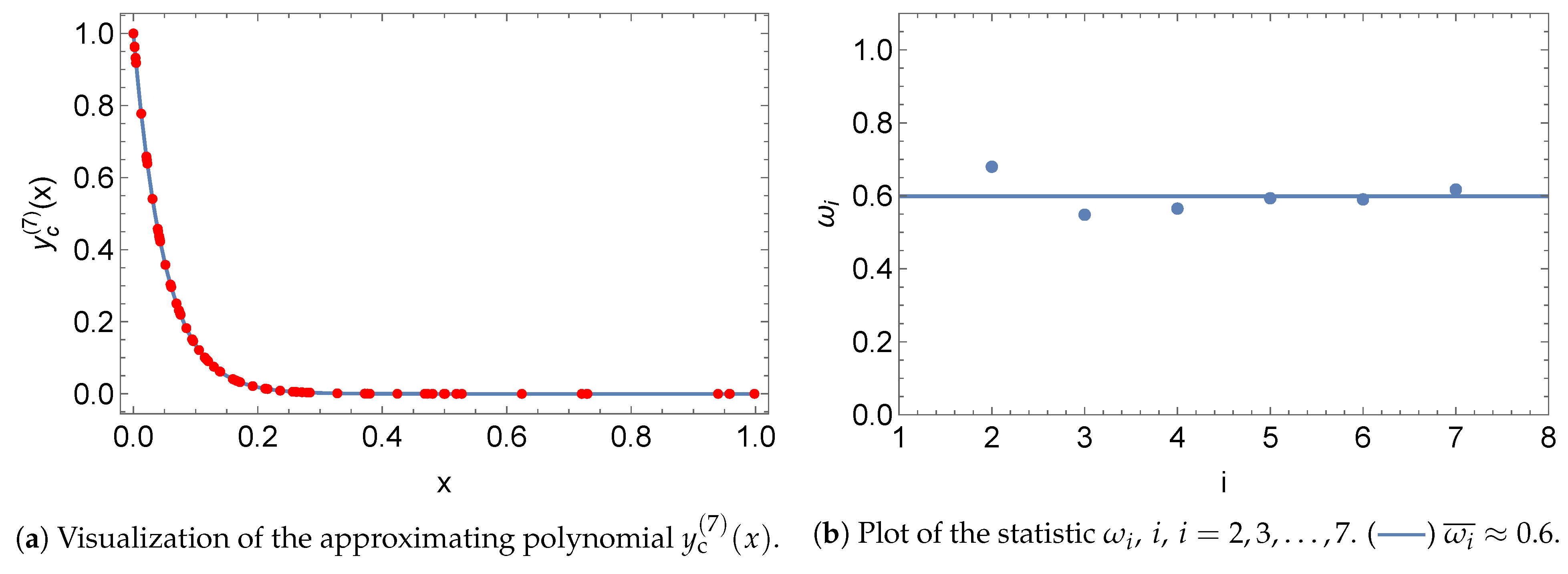
Figure 1. (a) The approximating polynomial y c ( 7 ) ( x ) . A proper subset of the set of points S is shown. (b) Plot of the statistic ω i . () ω i ¯ 0.6 .
Algorithms 15 00320 g001
Figure 2. (a) Fitting the upper bound (24) with the set R . (b) Visualization of the residual, absolute local approximation error, and the mean value.
Algorithms 15 00320 g002
Figure 3. The approximating polynomial y c ( 3 ) ( x ) . A proper subset of the set of points S is shown.
Algorithms 15 00320 g003
Figure 4. (a) Fitting the upper bound (24) with the set R . (b) Visualization of the residual, absolute local approximation error and the mean value.
Algorithms 15 00320 g004
Figure 5. (a) The approximating polynomial y c ( 10 ) ( x ) . A proper subset of the set of points S is shown. (b) Plot of the statistic ω i . () ω i ¯ 0.64 .
Algorithms 15 00320 g005
Figure 6. (a) Fitting the upper bound (24) with the set R . (b) Visualization of the residual, absolute local approximation error, and the mean value.
Algorithms 15 00320 g006
Figure 7. (a) Fitting the upper bound (24) with the set R . (b) Visualization of the residual, absolute local approximation error, and the mean value.
Algorithms 15 00320 g007
Figure 8. Visualization of the approximating polynomial and statistic ω i . (a) Approximating polynomial y c ( 9 ) ( x ) obtained by multiplying Equation (25) by x. (b) Approximating polynomial y c ( 8 ) ( x ) obtained by y ( x ) y c ( x ) . (c) Plot of ω i , i = 2 , 3 , , 9 . () ω i ¯ 0.66 . (d) Plot of ω i , i = 2 , 3 , , 8 . () ω i ¯ 0.61 .
Algorithms 15 00320 g008
Figure 9. (a) Fitting the upper bound (24) with the set R . (b) Visualization of the residual, absolute local approximation error, and the mean value.
Algorithms 15 00320 g009
Figure 10. Visualization of the approximating polynomial and the statistic ω i . (a) Approximating polynomial y c ( 7 ) ( x ) obtained from multiplying Equation (25) by x. (b) Approximating polynomial y c ( 6 ) ( x ) obtained from y ( x ) y c ( x ) . (c) Plot of ω i , i = 2 , 3 , , 7 . () ω ˜ i 0.49 . (d) Plot of ω i , i = 2 , 3 , , 6 . () ω i ¯ 0.58 .
Algorithms 15 00320 g010
Figure 11. (a) The approximating polynomial y c ( 8 ) ( x ) . A proper subset of the set of points S is shown. (b) Plot of the statistic ω i . () ω i ¯ 0.65 .
Algorithms 15 00320 g011
Figure 12. (a) Fitting the upper bound (24) with the set R . (b) Visualization of the residual, absolute local approximation error, and the mean value.
Algorithms 15 00320 g012
Figure 13. (a) The approximating polynomial y c ( 9 ) ( x ) . A proper subset of the set of points S is shown. (b) Plot of the statistic ω i . () ω i ¯ 0.62 .
Algorithms 15 00320 g013
Figure 14. (a) Fitting the upper bound (24) with the set R . (b) Visualization of the residual, absolute local approximation error, and the mean value.
Algorithms 15 00320 g014
Figure 15. Plotting the set R for m = 2 N + 1 = 5 Sinc points () and m = 2 N + 1 = 7 Sinc points ().
Algorithms 15 00320 g015
Figure 16. (a) The approximating polynomial y c ( 15 ) ( x ) . A proper subset of the set of points S is shown. (b) Plot of the statistic ω i . () ω i ¯ 0.46 .
Algorithms 15 00320 g016
Figure 17. (a) Fitting the upper bound (24) with the set R . (b) Visualization of the residual, absolute local approximation error, and the mean value.
Algorithms 15 00320 g017
Figure 18. (a) The approximating polynomial y c ( 16 ) ( x ) . A proper subset of the set of points S is shown. (b) Plot of the statistic ω i .
Algorithms 15 00320 g018
Figure 19. (a) Fitting the upper bound (24) with the set R . (b) Visualization of the residual, absolute local approximation error, and the mean value.
Algorithms 15 00320 g019
Table 1. Comparison of the L 2 norm of the approximation error for different methods.
MethodAdaptive PW PS[28]([65] Table 13(g))
y ( x ) y method ( x ) 1.104 × 10 14 3 × 10 5 1.9 × 10 12
Table 2. Comparison of the supremum norm of the approximation error for different methods.
MethodAdaptive PW PS[67]
y ( x ) y method ( x ) 1.215 × 10 10 4.3 × 10 10
Publisher’s Note: MDPI stays neutral with regard to jurisdictional claims in published maps and institutional affiliations.