Article

Traffic Demand Estimations Considering Route Trajectory Reconstruction in Congested Networks

1
College of Automobile and Traffic Engineering, Nanjing Forestry University, Nanjing 210037, China
2
School of Automotive and Traffic Engineering, Jiangsu University, Zhenjiang 212013, China
*
Author to whom correspondence should be addressed.
Algorithms 2022, 15(9), 307; https://doi.org/10.3390/a15090307
Submission received: 11 August 2022 / Revised: 25 August 2022 / Accepted: 25 August 2022 / Published: 28 August 2022

Abstract

:
Traffic parameter characteristics in congested road networks are explored based on traffic flow theory, and observed variables are transformed to a uniform format. The Gaussian mixture model is used to reconstruct route trajectories based on data regarding travel routes containing only the origin and destination information. Using a bi-level optimization framework, a Bayesian traffic demand estimation model was built using route trajectory reconstruction in congested networks. Numerical examples demonstrate that traffic demand estimation errors, without considering a congested network, are within ±12; whereas estimation demands considering traffic congestion are close to the real values. Using the Gaussian mixture model’s technology of trajectory reconstruction, the mean of the traffic demand root mean square error can be stabilized to approximately 1.3. Traffic demand estimation accuracy decreases with an increase in observed data usage, and the designed iterative algorithm can predict convergence with 0.06 accuracy. The evolution rules of urban traffic demands and road flows in congested networks are uncovered, and a theoretical basis for alleviating urban traffic congestion is provided to determine traffic management and control strategies.

1. Introduction

With the accelerated development of urbanization in developing countries, such as China, car ownership has increased substantially, triggering a surge in urban traffic. It is difficult for limited traffic routes to meet the rapid growth in urban traffic demand, resulting in disordered and congested urban traffic. However, car ownership is not proportional to urban congestion. In other words, urban congestion can be alleviated through rational planning of urban road networks and effective formulation of traffic control policies.
Origin–destination (OD) demand, which describes the distribution characteristics of traffic travel space, is an important input parameter for long-term urban traffic planning and short-term traffic management. OD demand is helpful in traffic network design (with respect to traffic bottleneck identification, road network capacity assessment, etc.) and traffic demand management (with respect to road congestion pricing, traffic control, etc.) in congested networks [1]. Therefore, accurately estimating OD demand can help ascertain traffic characteristics of current road networks, facilitating alleviation of traffic congestion in a more targeted and purposeful way during traffic planning and urban planning [2].
In recent years, transportation scholars have increasingly focused on OD demand estimation [3], especially regarding new data sources, methods, and theories associated with the theoretical and practical research of transportation planning. Existing studies can be categorized as OD demand estimation for either non-congested or congested networks (depending on the application’s scope) and as static or dynamic OD demand estimation (depending on whether time variations are considered). Maximum entropy theory has been employed to estimate traffic demand for non-congested networks based on observing link flow [4]. Hazelton [5] further estimated OD demand based on the Bayesian method. Parry and Hazelton [6] observed link flow and route flow at the same time, and estimated traffic demand using the maximum likelihood method. The Kalman filtering method has been dynamically used to predict the OD demand for rail transit [7]. Some scholars determined traffic demand based on the generalized least square method by observing information such as link flow, route flow, speed, and entrance lane flow at intersections [8,9]. Grange et al. used maximum entropy theory to estimate traffic demand on congested networks based on observing vehicle density at links [10]. Many scholars observed variables such as link flow, speed, and density to estimate traffic demand based on the generalized least square method [11,12,13]. Many OD demand estimation models use other theoretical frameworks, including OD demand estimation under supervised learning, sub-network OD demand estimation [14], OD demand estimation based on mobile phone location data [15], OD demand estimation based on bus card data [16], and multi-target OD demand estimation models [17].
The main weaknesses of current OD demand estimation research are as follows. (1) Existing studies ignore congestion characteristics in the observed travel data of road networks of various types. (2) The existing traffic demand estimation literature usually only includes road traffic data location and time information for origin and destination, lacking route trajectory reconstruction research. (3) Although road detection equipment can monitor a large amount of route travel time data, the existing Bayesian traffic demand estimation method fails to integrate the route travel time. This paper further reconstructs route trajectory data and establishes a Bayesian traffic demand estimation model with route trajectory reconstruction in congested networks by analyzing the propagation mechanism of congested traffic parameters and transforming the multi-source observed variables to a uniform format. Next, an iterative algorithm designed to solve the model is presented. Finally, numerical experiments are employed to test the model and algorithm.

2. Observed Data Analysis and Processing

In this section, the functional relationship between traffic flow and travel time is resolved based on the analysis of congested networks’ traffic characteristics. Multi-source observed variables are transformed to a uniform format, and further trajectory of observed route data is reconstructed using cluster analysis technology.

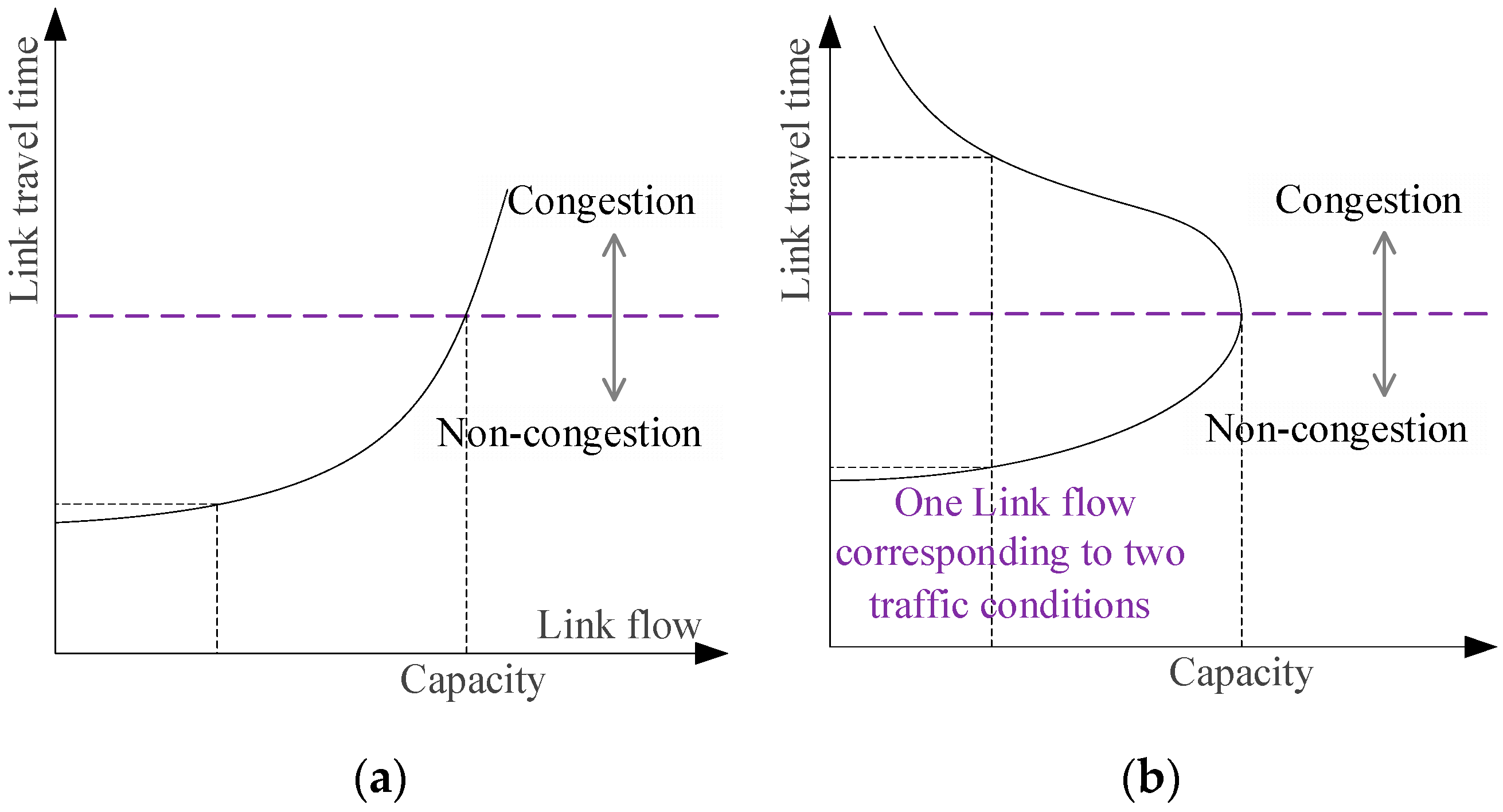
2.1. Analysis of Traffic Congestion Characteristics

Traditional OD estimation methods in congested networks assume that link travel time increases monotonically with link flow (as shown in Figure 1a). However, in actual urban networks, link travel time is a non-monotony and non-convex function of link flow [18], and each link flow value corresponds to two different road conditions (as shown in Figure 1b). Therefore, traditional methods using link characteristic functions, which are increasing monotonical, is not suitable for OD demand estimation in congested networks; function errors might propagate to output results, which reduces the reliability of traffic network planning and design. There is a one-to-one correspondence between road travel time and traffic flow; therefore road travel time can be used as an effective observed variable for traffic demand estimation in congested networks.

2.2. Unification of Traffic Variables’ Dimensions

Modern information technology (such as automatic vehicle identification technology and GPS positioning technology) drives the development of traffic detectors. Different periods and types of traffic data can be observed, such as link traffic flow, speed, density, travel time, etc. The inconsistencies of dimension between these observed variables affect further application of data. As noted above, there are analytical relations among link flow, speed, and travel time in congested networks. Therefore, traffic flow theory is adopted to transform the dimension of observed variables to unify observed multi-source link information. In this paper, the Green Shields traffic flow–speed–density relation function was used to unify multi-source observed variables in link travel time [19]. In other words, the inverse function of Equation (1) was used to transform the dimension of each traffic flow parameter relationship:
v a = l a t a [ M j , a ( 1 l a t a S f , a ) ] , a A
where A represents set of links, a A ; v a represents traffic volume of link a ; t a represents estimated travel time of link a ; l a represents length of link a ; M j , a represents congestion density of link a ; and S f , a represents maximum driving speed of link a . Link travel time can be derived from link length and vehicle speed.

2.3. Route Trajectory Reconstruction Based on Gaussian Mixture Clustering Analysis

Usually, only origin and destination information of a travel route can be obtained during the monitoring process of actual traffic data. For example, automatic vehicle identification data and mobile phone bill data can only capture trip start and end time and location information. Therefore, route trajectory reconstruction of such data is required for traffic demand estimation.
The Gaussian mixture model is a soft data clustering method, which can effectively describe the distribution of the mixed density function of observed data [20]. In the process of route trajectory reconstruction, observed travel route information with the same origin and destination are subject to a set of probability distributions with unknown mean and variance. Each observation (trajectory unknown) is a sample of multi-model distribution. Next, the probability density function of the Gaussian mixture model is formed using the probability density function corresponding to multiple sets of origin and destination points. Equations (2)–(4) build a route trajectory reconstruction model based on Gaussian mixture clustering analysis:
max L ( c , σ , π ) = i I log ( k K ω π k ω N ( x ^ i | c k ω , σ k ω 2 ) )
Constraints are:
k K ω π k ω = 1 , ω W
0 π k ω 1 , k K ω , ω W
where I represents the set of observed routes (trajectory unknown) i I ; X ^ i represents the ith observed route travel time; W is the set of OD pairs of the road network, ω W ; K ω represents the set of all routes in OD pairs ω , k K ω ; π k ω is the mixing weight of the route k in OD pair ω , and k K ω π k ω = 1 , ω W ; c k ω represents the expected value of travel time of the route k in OD pair ω ; σ k ω 2 represents the variance in travel time of the route k in OD pair ω ; N ( x ^ i | c k ω , σ k ω 2 ) represents the probability density function of Gaussian distribution with mean c k ω and variance σ k ω 2 at X ^ i . Objective function (2) represents the maximized Gaussian mixture likelihood function. Constraints (3)–(4) are mixed weight conservation and interval constraint, respectively.
Thus, route travel time after trajectory reconstruction can be obtained using:
x i = k K ω γ k , i ω c k ω , i I
In the following formula, γ k , i ω represents the weight coefficient of the coincidence between the ith observed travel trajectory and the route k in OD pair ω .
γ k , i ω = π k ω N ( x ^ i | c k ω , σ k ω 2 ) k K ω π k ω N ( x ^ i | c k ω , σ k ω 2 ) , k K ω , ω W , i I

3. A Bayesian Traffic Demand Estimation Model Using Route Trajectory Reconstruction in Congested Networks

3.1. Analysis of the Relationship between Traffic Demand and Observed Variables

Travelers’ choice of travel destination and driving route can be regarded as a large number of independent Bernoulli experiments. Therefore, this paper assumes that the traffic demand follows the multivariate normal distribution, D ~ MVN ( μ D , Σ D ) , with mean vector μ D and covariance matrix Σ D . Traffic demand varies in different time periods and weather conditions. For example, traffic demand increases during holidays and decreases in severe weather conditions. In order to describe these characteristics, this paper adopts the following form of traffic demand:
D ω = k ω U + η ω
where k ω describes the relative weight that the demand of OD pairs ω account for total traffic demand, and k is its vector form, namely k = { , k ω , } . U reflects the changing situation of traffic demand over time and weather, and follows the normal distribution form of mean μ U and variance σ U 2 . η ω is random errors which are mutually independent, and follows the normal distribution form of mean 0 and variance σ η 2 , and η is its vector form, namely η = { , η ω , } .
Considering the conservation relationship between link flow and OD demand:
v a = ω W k K ω p k ω δ a , k ω d ω , a A
where v a represents traffic flow of link a and δ a , k ω represents the associated parameter of route-link among OD pairs ω , if link a is on route k , the parameter is 1; otherwise, the parameter is 0. p k ω represents travelers’ route choice probability on route k in OD pair ω , which can be obtained by solving the following stochastic user equilibrium (SUE) model:
p k ω = exp ( θ c k ω ) k exp ( θ c k ω ) , k K ω , ω W
where θ is a discrete parameter used to measure the perception error degree of travelers; and c k ω represents the estimated route travel time on route k in OD pair ω .
β a ω = k p k ω δ a , k ω represents the ratio between the number of drivers using link a and the demand of OD pairs, where β is all OD-link ratio matrix. Thus, Equation (8) can be written as:
v a = ω W β a ω d ω , a A
To reduce the solving complexity of the Bayesian estimation model, the first-order Taylor expansion of road impedance function replaces link travel time. As the designed algorithm is iterative, the error generated by the replacement in the iterative algorithm gradually decreases. According to the link congestion and impedance function (Equation (1)), link travel time can be deduced as:
t a = m a v a + n a = m a ω W k K ω p k ω δ a , k ω d ω + n a , a A
where m a and n a are the coefficients of first-order Taylor expansion. Further, route travel time can be written as:
c k ω = a A δ a , k ω t a , k K ω , ω W

3.2. Model Establishment

The principle of Bayesian traffic demand estimation is to correct the prior OD demand distribution according to the observed data (including data after dimension unification of congested road networks and route travel time after trajectory reconstruction), to obtain the posterior OD demand distribution. Bayesian estimation methods use both observed information and historical information; a large amount of information helps to estimate more reliable traffic demand. The model expression is the following bi-level programming form.
The upper-level:
D ˜ = arg max D f ( C ^ | D ) p ( D )   f ( C ^ | D ) p ( D ) d D
Constraint conditions: Formulas (7), (11) and (12).
The lower-level: Traffic demand D is allocated using the SUE model to obtain the OD-link ratio, β , and road flow properties m a and n a .
f k ω = q ω p k ω ( c ω ) = q ω Pr ( c k ω c l ω , l K ω , l k | c ω ) , ω W , k K ω
where C ^ represents the vector form of the processed observed data, C ^ = { , c ^ s , } , including t a of Equation (1) after dimension unification and x i of Equation (5) after trajectory reconstruction; Pr ( ) represents the probability operator; and c ω is the vector form of route travel time c k ω , namely c ω = { , c k ω , } . Formula (9) can be used to calculate p k ω . In the upper-level model of the bi-level programming framework, the objective function (13) is the maximum posterior probability estimation of the traffic demand under road data observation. Maximum posterior probability is used to obtain the point estimation value of traffic demand. The lower-level model of the bi-level programming framework estimates variables in the upper-level model constraints, namely the OD-link ratio and road flow properties.

4. Solving Algorithm

When solving the Gaussian mixture model, expectation maximization algorithm (EM) [21]. is used to calculate c k ω , σ k ω 2 , and π k ω in order. The mean c k ω and variance σ k ω 2 of route travel time are the extreme points of the Gaussian mixture model; that is, the partial derivatives of Equation (2) at c k ω and σ k ω 2 are zero:
L c k ω = 0 , k K ω , ω W
L σ k ω 2 = 0 , k K ω , ω W
According to the KKT optimality conditions of Formulas (2)–(4), mixing weight is calculated as follows:
π k ω = i I ω γ k , i ω | I ω | , k K ω , ω W
where | I ω | is the potential of set I ω .
As prior traffic demand is subject to multivariate normal distribution and all variables are linearly related (Equations (7), (11), and (12)), the Bayesian posterior distribution of unobserved variables (traffic demand) is also subject to multivariate normal distribution after observing some variables (road travel data) where the mean vector μ D | Z = C ^ and covariance matrix Σ D | Z = C ^ , respectively, are [22]:
μ D | Z = C ^ = μ D + Σ D Z Σ Z Z 1 ( C ^ μ Z )
Σ D | Z = C ^ = Σ D D Σ D Z Σ Z Z 1 Σ Z D
where Z represents all observed variables’ vectors. Therefore, the established upper-level model can be solved by updating Formulas (18) and (19). At each moment, the Bayesian traffic demand estimation model in congested environments was solved using the iterative algorithm framework, and the lower-level SUE model was solved using the method of successive averages (MSA). The designed algorithms for proposed model are as Algorithm 1.
Algorithm 1 The designed algorithms for proposed model
StepContents
1Initialization: Set the number of iteration steps n = 0 , convergence accuracy ε , initial demand weight matrix k ( 0 ) , mean μ U and variance σ U 2 of traffic demand level, random error parameter σ η 2 , discrete parameters θ of traveler perception error; observed data, and observed route travel time x ^ i .
2According to Equation (1), the observed variables are transformed to a uniform format to obtain the link travel time t a .
3The EM algorithm is used to solve c k ω , σ k ω 2 , and π k ω to determine the observed route trajectory.
(a) Initialize the mean c k ω , variance σ k ω 2 , and mixing coefficient π k ω of route travel time;
(b) Calculate the probability γ k , j ω using Equation (6);
(c) Use Equations (15) and (16) to update the mean c k ω and variance σ k ω 2 according to the current γ k , j ω , update the mixing coefficient π k ω according to Equation (17);
(d) If the parameter γ k , j ω converges (that is, the difference between the parameters of two iterations reaches convergence accuracy), the algorithm ends. Otherwise, go to step (b);
(e) Determine the observed route trajectory; that is, calculate x i using Equation (5).
4Solve the lower-level model: apply the MSA algorithm to solve the SUE model; that is, allocate the requirements D ( n ) , to obtain the OD-link ratio β ( n ) , m a , and n a .
5Solve the upper-level model: substitute the OD-link ratio β ( n ) , m a , and n a . According to Equations (18) and (19), successively use observed data to solve the auxiliary OD demand D ¯ ( n ) .
(a) Initialization: Set the initial update step number s = 0 . Observe the data dimension s max and calculate the prior mean vectors μ ( 0 ) and covariance matrices Σ ( 0 ) of all variables.
(b) According to the processed observed data c ^ s , use Equations (18) and (19) to update the posterior mean vector μ D | Z = v ^ s and covariance matrix Σ D | Z = c ^ s of all variables, and let μ Z | Z = c ^ s = c ^ s , Σ Z | Z = c ^ s = 0 , μ ( s ) = μ D | Z = c ^ s , and Σ ( s ) = Σ D | Z = c ^ s .
(c) Convergence test: let s = s + 1 ; if s s max , stop the calculation, and let D ¯ ( n ) = μ ( s ) . Otherwise, go to step (b).
6Update traffic demand: let D ( n + 1 ) = D ( n ) + 1 / ( n + 1 ) ( D ¯ ( n ) D ( n ) ) .
7Convergence test: if D ( n + 1 ) D ( n ) / D ( n ) ε , stop the calculation, and D ( n + 1 ) is the optimal traffic demand. Otherwise, let n = n + 1 , and go to Step 3.

5. Numerical Experiment

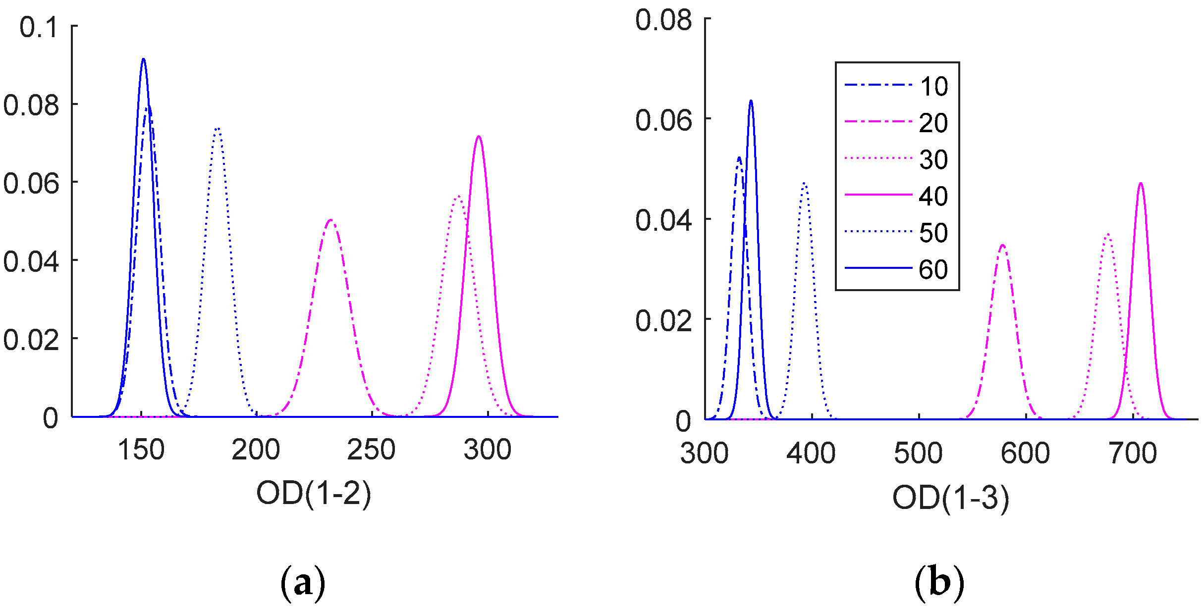
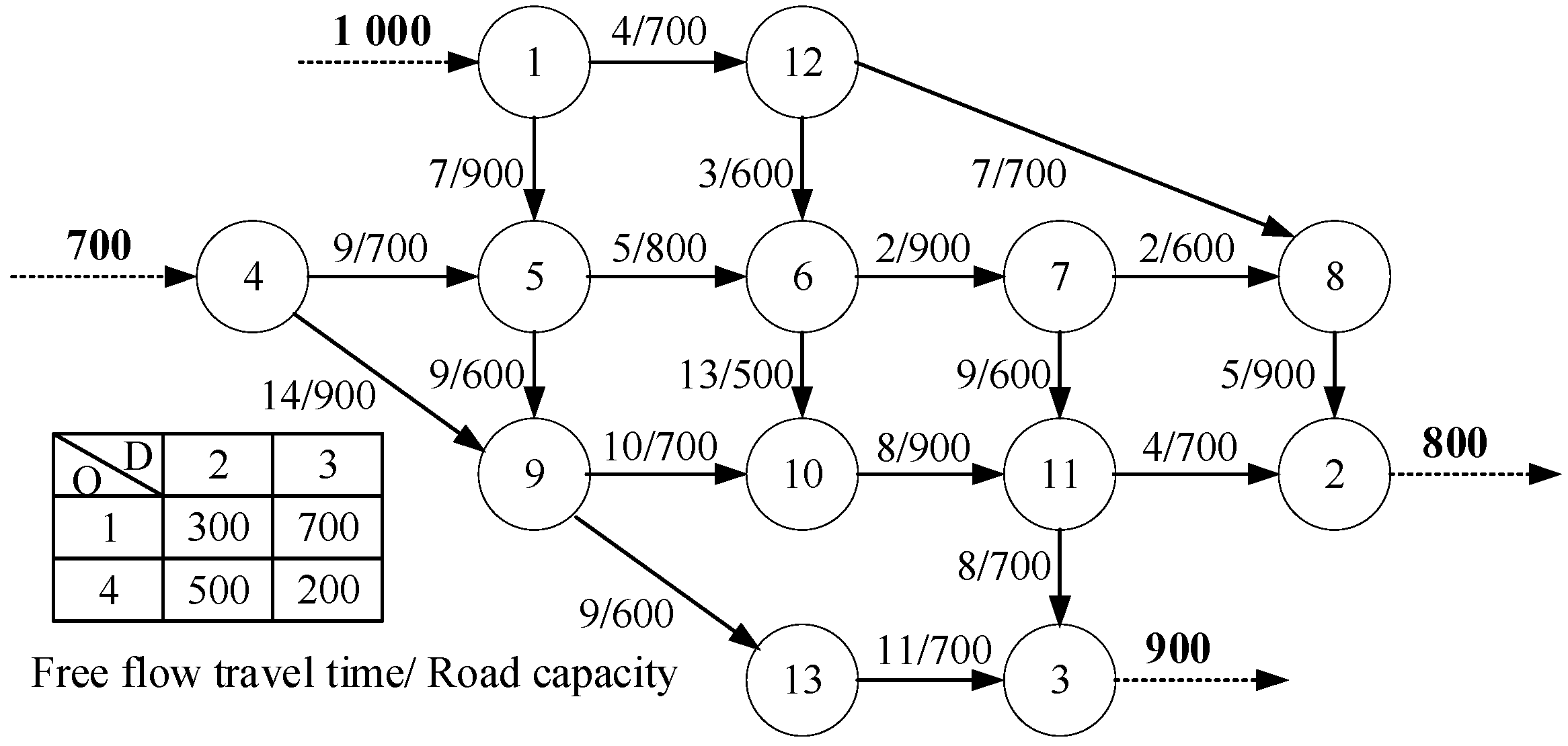
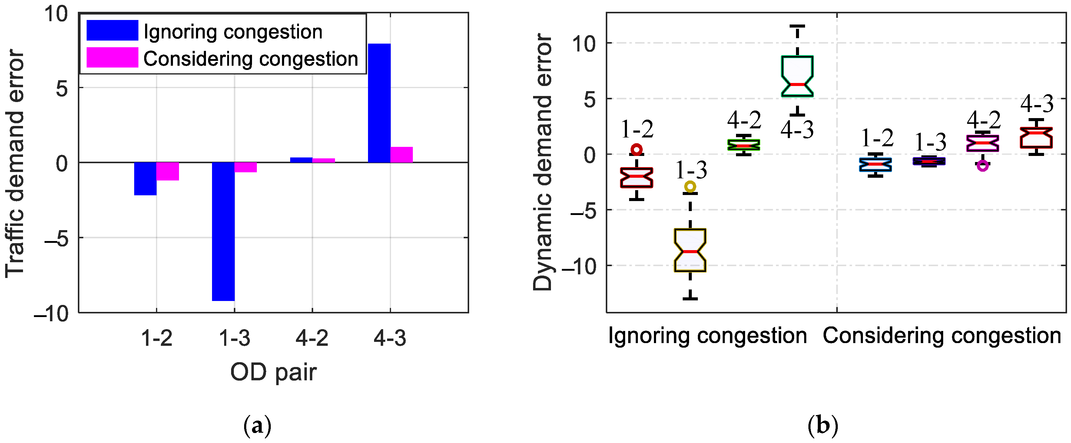
5.1. Nguyen–Dupuis Network

Topology structures, road properties and traffic demand of the Nguyen–Dupuis network [23] are shown in Figure 2. Traffic demand in the figure is d ω = k ω U , and traffic operation status of 60 time windows within two hours is observed using Vissim simulation technology, where traffic demand in the first half hour and the last half hour is set as 1 / 2 d ω , and traffic demand in the middle hour is set as d ω . Each time window captured 50 groups of link flow, 30 groups of link travel time, and 20 groups of route travel time with unknown trajectories. The congested links are set as 5-6, 6-7, 10-11, and 11-2, and the maximum driving speed S f , a of each link is 40. According to the Green Shields model, the link length and value of congestion density in Equation (1) are: (free flow travel time × maximum driving speed) and (4 × road capacity/maximum driving speed), respectively. Traffic demand variance is σ U 2 = 10 . The initial demand weight matrix is k ( 0 ) = [ 6 , 10 , 8 , 6 ] . Random error parameters are not considered. The discrete parameter of traveler perception error is set as θ = 1 .
The learning process of the Bayesian traffic demand estimation model solution in a congested environment was tested. Figure 3 depicts the distribution status of traffic demand in the 10th, 20th, 30th, 40th, 50th, and 60th time windows, respectively, where the abscissa is the number of the OD demand and the ordinate is the probability that the OD demand is the corresponding value. Different colors and lines represent testing different time windows (see Figure 3b). Note that the predicted traffic demand of the first and last half hours (the 10th, 50th, and 60th time windows) is lower, and the traffic demand of the middle hour (the 20th, 30th, and 40th time windows) is higher. In the 20th time window, the variance in traffic demand is relatively large, because the traffic demand has just changed from 1 / 2 d ω to d ω , and observed data makes a significant difference. After traffic demand stabilizes, its variance is low (the 60th period, for example). Figure 3 also shows that the proposed model can reflect the change state of real-time traffic demand.
Bayesian traffic demand estimation models for estimated errors under cases when traffic congestion is and is not considered are compared in Figure 4. Figure 4a depicts errors in traffic demand estimations in the 30th time window, and Figure 4b is the probability distribution of errors in traffic demand estimations in all 60 time windows. The ordinates in the graph are the differences between estimated traffic demand and actual traffic demand. Figure 4a illustrates that traffic demand estimations considering congestion are significantly superior to estimations ignoring congestion. Figure 4b illustrates that errors in traffic demand estimation without considering network congestion are within ±12, and that the average error in traffic demand estimations considering congestion is near zero. This is because traffic demand estimations ignoring congestion are based on monotonous road travel time increases with link flow, which violates actual traffic flow characteristics.
To illustrate the role of unknown route trajectory data in traffic demand estimations, root mean square errors of traffic demand with different observed data are shown in Figure 5. In Figure 5, we compare three cases: a trajectory reconstruction based on the Gaussian mixture model, a k-means clustering trajectory, and only integrating data with known trajectories. The root mean square error is defined as: R M S E = d t r u d e s t / | ω | , where d t r u , d e s t , and | ω | represent exact traffic demand, estimated traffic demand, and potential traffic demand (number of set elements), respectively. Compared with only integrating data with known trajectories, the root mean square error of traffic demand estimation is smaller, but its variance fluctuates significantly. Compared with the k-means clustering trajectory method, variance in the root mean square error of traffic demand estimations based on trajectory reconstruction using the Gaussian mixture model is larger, but the mean error stabilizes at approximately 1.3. Therefore, trajectory reconstruction using the Gaussian mixture model is more accurate for traffic demand estimation than using k-means cluster trajectory or only integrating data with known trajectories.

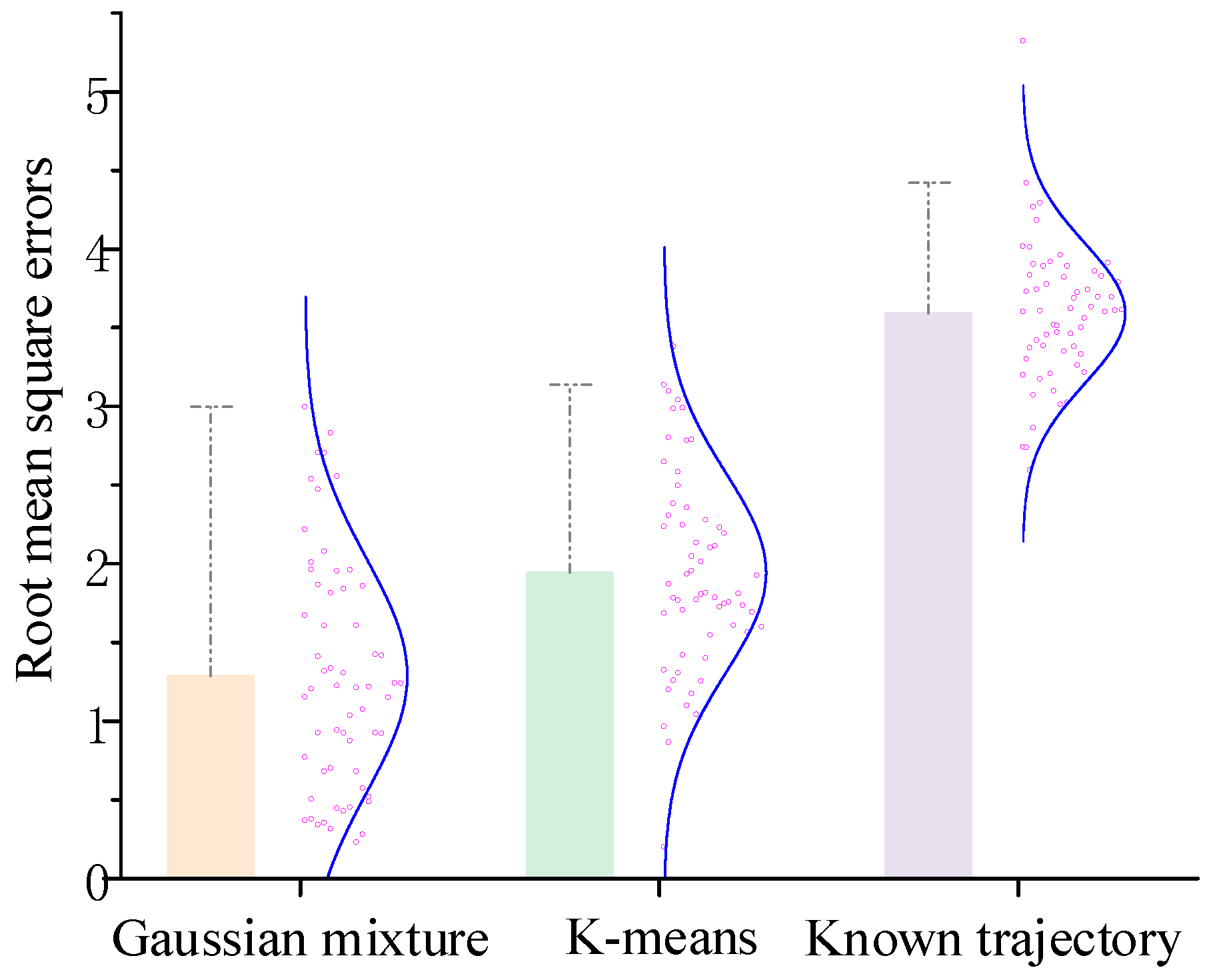
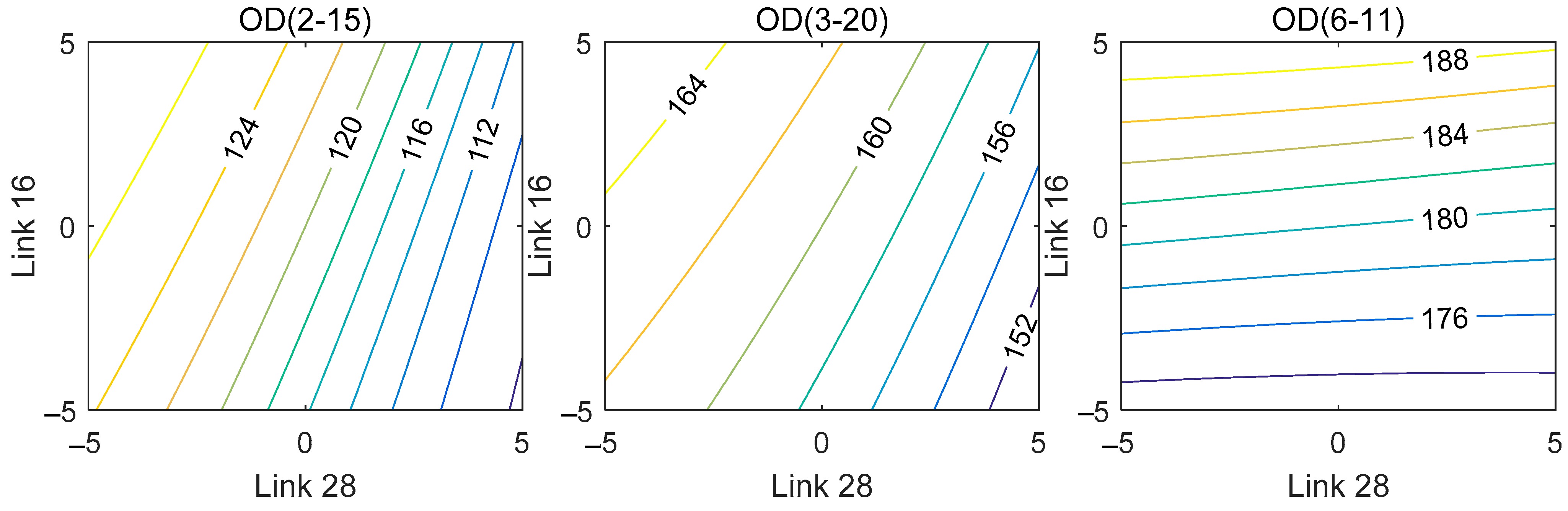
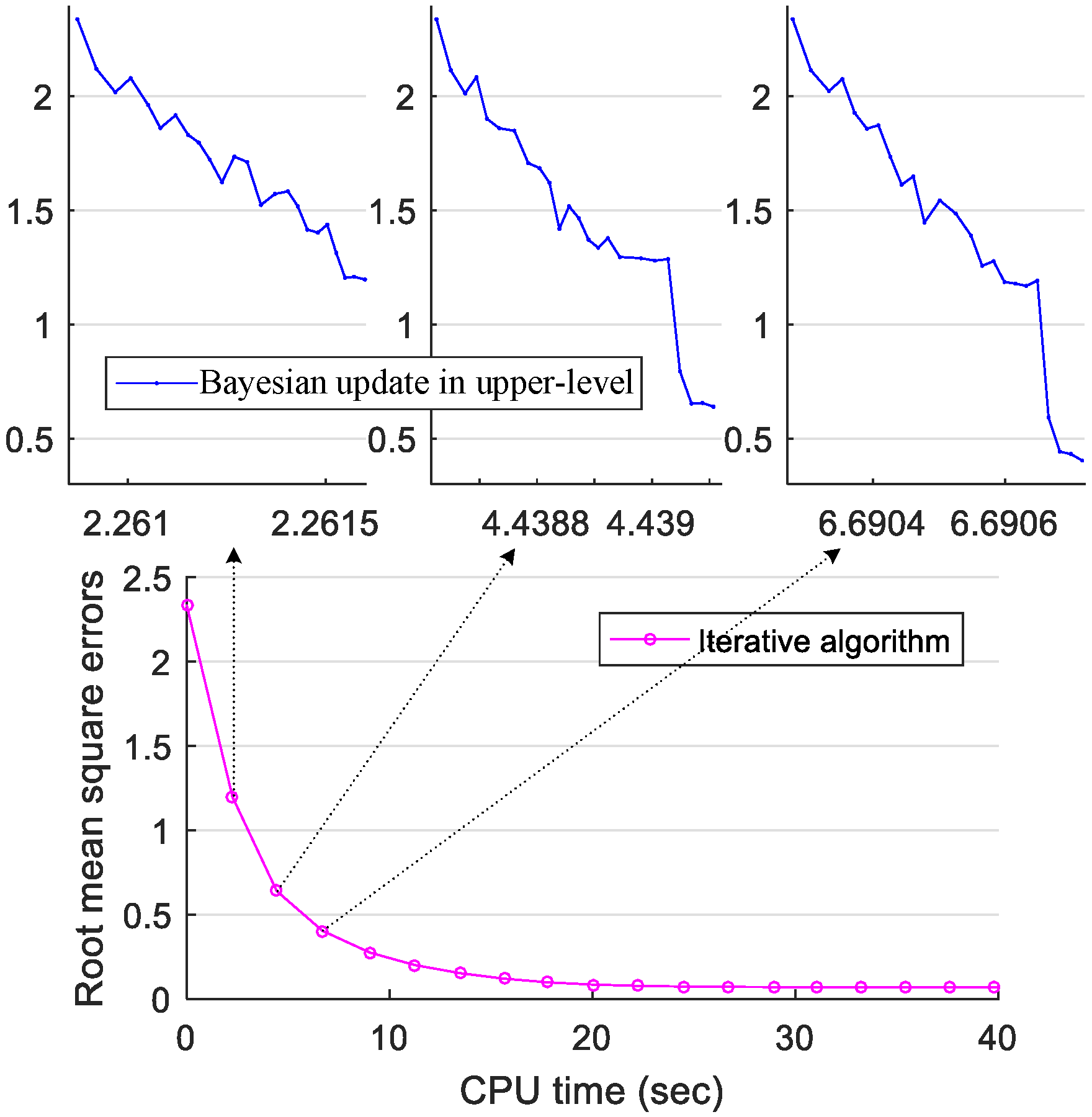
5.2. Sioux Falls Network

The Sioux Falls network [24] was used to further test the applicability of the designed algorithm. This road network consists of 24 nodes, 76 links, and 550 OD pairs. Characteristics of this road link are described in the literature [24]. Observed variables, link maximum driving speed, link length, and congestion density are consistent with the Nguyen–Dupuis network. The sensitivity of traffic demand to link observed data is shown in Figure 6. Observed traffic flow and speed on links 16 and 28 are disturbed, respectively. From these three figures, it can be seen that when the disturbance of observed variables is 0%, estimated traffic demand is close to its actual value (i.e., 120, 160, and 180). When disturbance increases, estimated traffic demand gradually diverges from actual demand. In this experiment, OD pairs 2-15 and 3-20 are more sensitive to observed data on link 28, whereas OD pair 6-11 is more susceptible to observed data on link 16.
The evolution process of the Bayesian traffic demand estimation algorithm with route trajectory reconstruction in congested networks was plotted, and is shown in Figure 7. The lower part of the figure illustrates a convergence situation of root mean square error of the entire iterative algorithm; the upper three figures represent the convergence process of the Bayesian update strategy (upper model) in the second, third, and fourth iterations of the algorithm, respectively. In the calculation process, the designed iterative algorithm and the Bayesian successive update method in the upper-level model can converge to accuracies of 0.06 and 0.003, respectively. The root mean square error of traffic demand decreases steadily during each iteration, whereas the root mean square error does not continue to decrease when solving the upper-level model. However, with an increase in observed information, the method ensures that the overall trend of root mean square error decreases. This indicates that the algorithm is robust.

6. Conclusions

In this paper, the relationship between traffic variables and travel characteristics in congested network environments is analyzed, and the Bayesian traffic demand estimation model with route trajectory reconstruction in congested networks is established. Data analysis of traffic environments reveals that there is a non-monotone relationship between link travel time and traffic flow in congested networks. Therefore, the three-parameter relationship of congested network flow is analyzed to transform observed variables to a uniform format. The Gaussian mixture model is used to reconstruct observed route trajectories using location data of observed route trajectories. The Bayesian estimation method is used to estimate OD, to modify prior OD demand distribution using observed data, and to obtain the posterior OD demand distribution in the current moment. The upper-level model is a maximized posterior probability distribution model, and the lower-level model is a stochastic network-user equilibrium model. The upper-level model transmits traffic demand to the lower-level model, and the lower-level model transmits the OD-link ratio and road flow properties to the upper-level model.
The Nguyen–Dupuis and Sioux Falls networks were used to test the properties of the proposed model and algorithm. The results show that traffic demand estimations that consider traffic congestion are significantly better than those that ignore traffic congestion, with traffic estimation errors of almost 0 and within ±12, respectively. Compared with only integrating known trajectory data, the mean of root mean square error of traffic demand estimated by integrating unknown route trajectory data is smaller. Compared with the k-means clustering trajectory method, the mean of root mean square error of traffic demand estimated using the Gaussian mixture model reconstruction trajectory is smaller and stabilizes at approximately 1.3. The designed iterative algorithm and the Bayesian successive update method in the upper-level model can converge to 0.06 and 0.003, respectively.
The Bayesian traffic demand estimation model with route trajectory reconstruction in congested networks can be applied to urban traffic system optimization projects; a variety of traffic demand distribution forms are adopted to establish the traffic demand estimation model.

Author Contributions

Conceptualization, W.T., J.C. and C.S.; methodology, W.T., C.S. and G.L.; writing—original draft preparation, W.T., J.C., H.W. and C.S.; writing—review and editing, W.T. and C.S. All authors have read and agreed to the published version of the manuscript.

Funding

This study was supported by the Natural Science Fund for Colleges and Universities in Jiangsu Province under Grant 20KJB580016, the General Program of Philosophy and Social Science Research in Jiangsu Universities under Grant 2020SJA0133, the MOE of PRC Industry-University Collaborative Education Program (Program No. 202102055014, Kingfar-CES “Human Factors and Economics” Program), and the Science and Technology Innovation Fund for Youth Scientists of Nanjing Forestry University under Grant CX2018011.

Institutional Review Board Statement

Not applicable.

Data Availability Statement

Data used to support the findings of this study are available from the corresponding author upon request.

Conflicts of Interest

The authors declare no conflict of interest.

References

  1. Lou, Y.; Yin, Y.; Lawphongpanich, S. Robust congestion pricing under boundedly rational user equilibrium. Transp. Res. Part B Methodol. 2010, 44, 15–28. [Google Scholar] [CrossRef]
  2. Pan, Y. Lagrangian relaxation for the multiple constrained robust shortest path problem. Math. Probl. Eng. 2019, 2019, 3987278. [Google Scholar] [CrossRef]
  3. Zhou, X.; Mahmassani, H.S. A structural state space model for real-time traffic origin–destination demand estimation and prediction in a day-to-day learning framework. Transp. Res. Part B Methodol. 2007, 41, 823–840. [Google Scholar] [CrossRef]
  4. Willumsen, L.G. Estimation of OD matrix from traffic counts—A review. Working Paper. Inst. Transp. Stud. Univ. Leeds. 1978. Available online: https://www.semanticscholar.org/paper/ESTIMATION-OF-AN-O-D-MATRIX-FROM-TRAFFIC-COUNTS-A-Willumsen/87d6a7d6d04bc27ad23f422ae471f3d888481a8f (accessed on 10 August 2022).
  5. Hazelton, M.L. Bayesian inference for network-based models with a linear inverse structure. Transp. Res. Part B Methodol. 2010, 44, 674–685. [Google Scholar] [CrossRef]
  6. Parry, K.; Hazelton, M.L. Estimation of origin-destination matrices from link counts and sporadic routing data. Transp. Res. Part B Methodol. 2012, 46, 175–188. [Google Scholar] [CrossRef]
  7. Jiao, P.; Li, R.; Sun, T.; Hou, Z.; Ibrahim, A. Three revised kalman filtering models for short-term rail transit passenger flow prediction. Math. Probl. Eng. 2016, 2016, 9717582. [Google Scholar] [CrossRef]
  8. Yang, Y.; Fan, Y.; Wets, R.J.B. Stochastic travel demand estimation: Improving network identifiability using multi-day observation sets. Transp. Res. Part B Methodol. 2018, 107, 192–211. [Google Scholar] [CrossRef]
  9. Yin, C.; Wang, X.; Shao, C. Do the Effects of ICT Use on Trip Generation Vary across Travel Modes? Evidence from Beijing. J. Adv. Transp. 2021, 2021, 6699674. [Google Scholar] [CrossRef]
  10. Grange, L.; González, F.; Bekhor, S. Path flow and trip matrix estimation using link flow density. Netw. Spat. Econ. 2017, 17, 173–195. [Google Scholar] [CrossRef]
  11. Shafiei, S.; Saberi, M.; Zockaie, A.; Sarvi, M. Sensitivity-based linear approximation method to estimate time-dependent origin-destination demand in congested networks. Transp. Res. Rec. 2017, 2669, 72–79. [Google Scholar] [CrossRef] [Green Version]
  12. Ma, W.; Pi, X.; Qian, S. Estimating multi-class dynamic origin-destination demand through a forward-backward algorithm on computational graphs. Transp. Res. Part C 2020, 119, 102747. [Google Scholar] [CrossRef]
  13. Abdelghany, K.; Hassan, A.; Alnawaiseh, A.; Hashemi, H.; Information, R. Flow-based and density-based time-dependent demand estimation for congested urban transportation networks. Transp. Res. Rec. 2020, 2498, 27–36. [Google Scholar] [CrossRef]
  14. Sun, C.; Chang, Y.; Shi, Y.J.; Cheng, L.; Ma, J. Subnetwork origin-destination matrix estimation under travel demand constraints. Netw. Spat. Econ. 2019, 19, 1123–1142. [Google Scholar] [CrossRef]
  15. Krishnakumari, P.; van Lint, H.; Djukic, T.; Cats, O. A Data driven method for OD matrix estimation. Transp. Res. Part C Emerg. Technol. 2020, 113, 38–56. [Google Scholar] [CrossRef]
  16. Hussain, E.; Bhaskar, A.; Chung, E. Transit OD matrix estimation using smartcard data: Recent developments and future research challenges. Transp. Res. Part C 2021, 125, 103044. [Google Scholar] [CrossRef]
  17. Sun, W.; Shao, H.; Shen, L.; Wu, T.; Lam, W.H.; Yao, B.; Yu, B. Bi-objective traffic count location model for mean and covariance of origin-destination estimation. Expert Syst. Appl. 2021, 170, 114554. [Google Scholar] [CrossRef]
  18. Newell, G.F. Non-convex traffic assignment on a rectangular grid network. Transp. Sci. 1996, 30, 32–42. [Google Scholar] [CrossRef]
  19. Zhao, N.; Yu, L.; Zhao, H.; Guo, J.; Wen, H. Analysis of traffic flow characteristics on ring road expressways in Beijing: Using floating car data and remote traffic microwave sensor data. Transp. Res. Rec. 2009, 2124, 178–185. [Google Scholar] [CrossRef]
  20. Zivkovic, Z. Improved adaptive Gaussian mixture model for background subtraction. In Proceedings of the International Conference on Pattern Recognition; IEEE Computer Society: Washington, DC, USA, 2004; pp. 28–31. [Google Scholar]
  21. Dempster, A.P.; Laird, N.M.; Rubin, D.B. Maximum likelihood from incomplete data via the EM algorithm. J. R. Stat. Soc. 1977, 39, 1–38. [Google Scholar]
  22. Maher, M.J. Inferences on trip matrices from observations on link volumes: A Bayesian statistical approach. Transp. Res. Part B Methodol. 1983, 17, 435–447. [Google Scholar] [CrossRef]
  23. Nguyen, S.; Dupuis, C. An efficient method for computing traffic equilibria in networks with asymmetric transportation costs. Transp. 1984, 18, 185–202. [Google Scholar] [CrossRef]
  24. Leblanc, L.J. Mathematical Programming Algorithms for Large Scale Network Equilibrium and Network Design Problems. Ph.D. Thesis, Northwestern University, Evanston, IL, USA, 1973. [Google Scholar]
Figure 1. Performance function of link travel time. (a) Traditional assumption. (b) Actual situation.
Algorithms 15 00307 g001
Figure 2. Topology, link characteristics, and OD demands of the Nguyen–Dupuis network.
Algorithms 15 00307 g002
Figure 3. Probability distribution of Bayesian learning-based OD demands under different time intervals. (a) OD pair 1-2. (b) OD pair 1-3.
Algorithms 15 00307 g003
Figure 4. Comparison of traffic demand estimation errors when traffic congestion is and is not considered. (a) Traffic demand errors in the 30th time window. (b) Probability distribution of traffic demand errors in all time periods.
Algorithms 15 00307 g004
Figure 5. Root mean square errors of traffic demands with different observed data.
Algorithms 15 00307 g005
Figure 6. Traffic demands between different OD pairs under fluctuations of observed data on links 16 and 28.
Algorithms 15 00307 g006
Figure 7. Evolution processes of root mean square errors of traffic demands.
Algorithms 15 00307 g007
Publisher’s Note: MDPI stays neutral with regard to jurisdictional claims in published maps and institutional affiliations.

