SepFree NMF: A Toolbox for Analyzing the Kinetics of Sequential Spectroscopic Data

Abstract

This work addresses the problem of determining the number of components from sequential spectroscopic data analyzed by non-negative matrix factorization without separability assumption (SepFree NMF). These data are stored in a matrix M of dimension “measured times” versus “measured wavenumbers” and can be decomposed to obtain the spectral fingerprints of the states and their evolution over time. SepFree NMF assumes a memoryless (Markovian) process to underline the dynamics and decomposes M so that $M=WH$, with W representing the components’ fingerprints and H their kinetics. However, the rank of this decomposition (i.e., the number of physical states in the process) has to be guessed from pre-existing knowledge on the observed process. We propose a measure for determining the number of components with the computation of the minimal memory effect resulting from the decomposition; by quantifying how much the obtained factorization is deviating from the Markovian property, we are able to score factorizations of a different number of components. In this way, we estimate the number of different entities which contribute to the observed system, and we can extract kinetic information without knowing the characteristic spectra of the single components. This manuscript provides the mathematical background as well as an analysis of computer generated and experimental sequentially measured Raman spectra.

1. Introduction

The laboratory conditions of sequential data from spectroscopy experiments are often chosen in such a way that the processes can be assumed to be autonomous. In autonomous processes, only the initial states of the entire system determine its future. The Markov property, the lack of a memory, relates to the microstates of the system in the processes examined, i.e., what happens in detail (metaphorically, behind the curtains) is Markovian. These details are often not searched for.

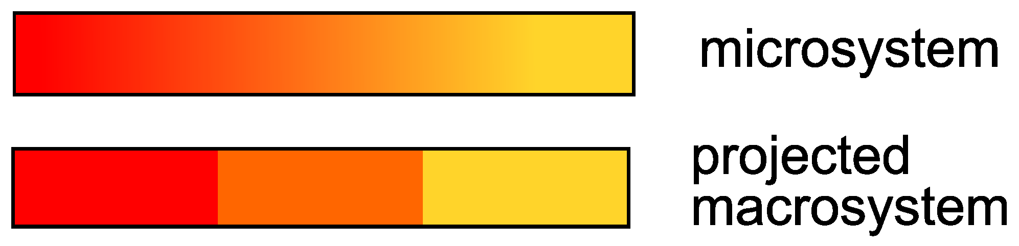
For instance, one could think of a toy-model reaction; in this reaction, a red solution gradually turns orange and then yellow with the time. By taking a picture of the solution with a certain time-step $\tau$, one observes the solution changing color. However, the exact nuance of the solution, e.g., the solution is orange-red, is not relevant for the experiment. Rather, one is interested only if the solution is red, orange or yellow. From the perspective of the solution, the overall system breaks down into three states; the Markov process, which takes places within the continuum of the colors that the solution can assume, is projected onto a three-dimensional space. A vector h, $h\in {\mathbb{R}}^{3\times m}$, indicates the proportion occupied by the colors red, orange and yellow in the overall system at each point in time of the measurement. This situation is displayed in Figure 1.

In other words, the solution has a memory because its color cannot “switch” from red to yellow within the interval $\tau$; if the solution is red, and it was dark red before, in the next time step it will be more likely orange-red, not yellow. Meanwhile, the particles in the solution can jump from red to yellow or to any color, regardless of the past particle color (Markov). If the Markov property were also met on the level of the projected macrosystem (the solution can be red-orange-yellow), one could find, e.g., an ordinary differential equation (a Markov process) matrix for the evolution of the concentration vectors. A solution of this system for fixed time-step $\tau$ could be represented by a matrix equation:

$$h_{t+\tau }^T=h_t^{T}K\left(\tau \right),$$

where the matrix $K\left(\tau \right)$ usually also depends on further quantities (e.g., temperature at which the reaction takes place), and $h^T\left(t\right)$ is the proportion of a state in the reaction. In the analysis of sequentially measured spectroscopic data, h is associated to a spectral fingerprint, as explained later in this work.

The transition from a micro to a macrosystem can have a systematic source of error, because a projected Markov system loses its Markov property.

Mathematically, there are two possibilities to model this “non-Markovianity”:

A

The process is assumed to have a memory. Not only the current (macro)state of the system, but also past steps of the process development have to be taken into account in order to derive a “forecast” for the future.

B

The clustering of microstates into coarser macrostates is assumed to be “fuzzy”. Then Markoviantity can be preserved, but we lose control about what we will denote as a macrostate.

Chemically, this article develops option B and presents a tool to compute the minimal past-time dependency of compounds in a reaction spectrum. A compound is a system’s state with an associated spectral fingerprint. The tool considers not only the compounds’ dependency on the past, which is called memory, but also the dependency in the kinetic development between the compounds themselves. This memory effect has been investigated in the mathematical context (e.g., [1,2]) and it has been observed in chemistry, for instance in the context of protein folding [3,4].

The interpretation of the compounds’ kinetics is more meaningful if the development of each kinetic curve is as independent as possible to the development of the other kinetic curves. A correlated development of kinetics causes an overlap of the kinetic curves. This is because they represent distinct physical system states and they are not chemical components.

The tool presented in the following measures the memory of the reaction compounds by scoring the overlap of the kinetic curves, following the theory of [5]. This analysis determines physical states corresponding to the basis vectors of an invariant subspace, as we will explain in the theory section. This way to compute the minimal memory effect is advantageous for spectral-data analysis, since it helps to determine the number of compounds in the reaction. If the number of compounds is too high, two or more compounds’ kinetic curves will overlap strongly since they are assigned to the same basis vector, or a linear combination of them.

Knowing the number of reaction compounds is important not only when analyzing the datasets, but also when performing experiments. In fact, the memory measure gives insights into the quality of the sample and the noise levels of the experimental setup.

The estimation of the minimal memory effect is possible with the SepFree NMF (separability-assumption free non-negative matrix factorization), a novel method based on the non-negative matrix factorization without separability assumption framework [6]. The non-negative matrix factorization without separability assumption is a matrix-decomposition method already used in the analysis of sequentially measured spectroscopic data. The structure of the datasets is the spectrum, in a certain wavenumber interval, measured for different times after the excitation of the sample. Furthermore, it is applicable also to time-resolved spectra; these investigate the evolution of photo-induced phenomena, as they measure the change of the optical signal (emission, absorption, Raman scattering) as a function of time (e.g., [7,8,9]).

This work uses the SepFree NMF for the analysis of the sequentially measured spectra. The method examines the sequentially measured spectrum as a matrix M to decompose into a product of matrix H, describing concentration proportions of the compounds as function of time, and matrix W, which describes the peak intensities of the compounds as function of wavenumber. In particular, the SepFree NMF models the evolution of the concentrations’ proportions of the compounds in H as a memoryless process, called the Markovian process [6].

A transition probability matrix matrix $K\left(\tau \right)$ governs the $\tau$-evolution of the columns of H:

$$\begin{array}{c}\hfill H_{t+\tau }^T=H_t^{T}K\left(\tau \right).\end{array}$$

(1)

The main contribution of this work is to provide a measure for the overlap between the rows of the concentration–proportion matrix H.

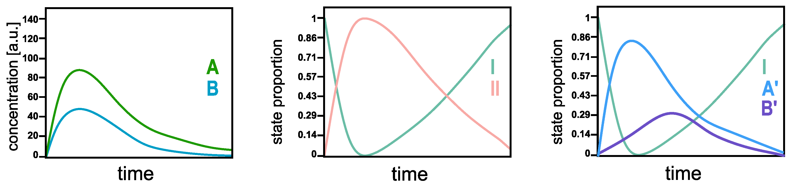
The SepFree NMF identifies the physical states of the system, not necessarily the chemical ones. In order to understand the difference, think of a reaction in which all the molecules can react into two compounds, A and B, and then go back to the initial state. In a standard multivariate curve resolution analysis [10], the concentration profile of the molecules in A and B evolves as in Figure 2 left. These curves represent the concentrations of A and B in the system as a function of time; they are not between 1 and 0. By SepFree NMF of rank 2, the algorithm returns the amount of system that is either is state I or in state II. Their time development will look as in Figure 2 middle. The first state I is the initial physical state of the system at the beginning of the reaction; all the molecules are in this state at time $t=0$, so its proportion will be (almost) 1. During the reaction, a second state II arises. This state II represents the amount of the system that is not in the initial condition I, that is, the amount of system molecules that is in either A or B. So, being in A or B is the second physical state of the system. By asking SepFree NMF for a decomposition into three physical compounds, the algorithm yields three states: the initial physical states, A’, and B’ (see Figure 2 right). Although the curves in Figure 2 right have a similar development to the concentration profiles in the left picture, their interpretation for the system is different. They represent the amount of the system that is in physical states A’ and B’, or in the initial state I, they are not concentration profiles.

This article is divided into three main parts. The first one explains the background of the SepFree NMF (Section 2.1), and of the PCCA+ projection (Section 2.2). The second part shows how we propose to compute the memory from the NMF results (Section 3). In the third part, we present examples of sequentially measured Raman spectra: first for computer-generated data, then for an experiment measuring the Raman spectrum of the crystallization process of paracetamol in methanol (Section 4).

2. Theoretical Foundations

Memory effects emerging from the projection of Markov micro processes to macro scales were discussed first with regard to mono- and multivalent binding events [11,12,13]. The resulting models provide a link for understanding macroscopic binding kinetics and to evaluate the strength and duration of the interaction of the ensemble molecules, facilitating the rational engineering of the binding dynamics.

It has been discussed whether and how these effects contribute to the binding rates of ligand–receptor systems [5]. The projection method to be applied is called non-negative matrix factorization (NMF).

2.1. SepFree NMF

SepFree NMF (separability-assumption free non-negative matrix factorization) is a novel method to decompose sequentially measured spectra. Decomposing the dataset into a matrix carrying the kinetic information and a matrix containing the peak intensities information is the first step for the computation of the memory effect of the compounds; this section briefly introduces the characteristics of the method.

The spectral dataset $M\in {\mathbb{R}}^{n\times m}$ consists of a spectrum measured at m time points and for n wavenumbers. Then, the matrix M contains the information about the dynamics of a number r of compounds. The SepFree NMF factorizes M into the multiplication of a matrix W, describing the peak intensities of the compounds, and a matrix H, describing their relative concentration proportions in the system as function of time [6]

$$\begin{array}{c}\hfill M=WH\end{array}$$

(2)

with the matrix $W\in {\mathbb{R}}^{n\times r}$ and the matrix $H\in {\mathbb{R}}_{+}^{r\times m}$. The matrix W represents r-component fingerprints as a function of the wavenumber.

Each of the r rows of the matrix H represents the proportion of the r-compounds as function of time t. Since H represents proportions of system’s states, its entries are required to be positive and between $[0,1]$. The column sum of H is a partition of unity.

Each of the r columns of the matrix W represents the intensity of a compound as a function of the wavenumber (or wavenumbers). With the standard ansatz, the matrix M has to be r-separable [14,15]. A matrix M is r-separable if there exists a factorization for which all r-columns of W are equal to a column of M [6]. This implies that a compound is present at least once as $100\%$ at a time t in the process described by M, while all the other compounds have a concentration of $0\%$ at t. However, in experiments, one measures always a mixture of compounds, and the forenamed situation in which a compound constitutes the entire system is not realistic. If only one compound is present at a specific time, then all the sample molecules would be in the same condition at that point in time.

Thus, the auxiliary of the separability assumption makes this algorithm particularly appropriate for the analysis of experimental data.

The authors of [6] model the time evolution of the columns in H as a Markov process. The evolution of the compounds at time $t+\tau$ depends only on the conditions at time t, and it is given by (1), whereby $K\in {\mathbb{R}}^{r\times r}$ is a row-stochastic transition matrix. Its elements $K{\left(\tau \right)}_{ij}$, $i,j=1,\dots ,r$, describe the transition probability from i to j after a time-step $\tau$. In this model, $K\left(\tau \right)$ is fixed for the time interval $\tau$. The transition probability in the process does not explicitly depend on time, and the process is said to be autonomous [16].

The factorization of the matrix M as a product of W and H has not a unique solution [17]. One can find a set of solutions, but not all the solutions of this set will satisfy the necessary conditions the decomposition has to have to represent the system. To select the decomposition that better reconstructs the data matrix M from the set of solutions, a penalty function $\mathsf{\Psi }$ is defined [6]. This function weights the required structural properties of the decomposition; the optimal solution for the decomposition of M is obtained by minimizing the value of $\mathsf{\Psi }$. The requirements the obtained matrices have to meet are five:

• The entries of W are non-negative;
• The entries of H are non-negative;
• H is column-stochastic;
• The entries of K are non-negative;
• K is row-stochastic.

To simplify the reading, we drop the $\tau$ of $K\left(\tau \right)$. These five requirements are then incorporated in the objective function $\mathsf{\Psi }$, defined as follows:

$$\begin{array}{c}\hfill \mathsf{\Psi }=\alpha \left(\underset{i,j}{min}{W}_{ij}\right)+\beta \left(\underset{i,j}{min}{H}_{ij}\right)+\gamma \left(\underset{j}{max}\mid 1-\sum _i^r{H}_{ij}\mid \right)\\ \hfill +\delta \left(\underset{i,j}{min}{K}_{ij}\right)+\mu \left(\underset{i}{max}\mid 1-\sum _j^r{K}_{ij}\mid \right),\end{array}$$

(3)

where the coefficients $\alpha ,\beta ,\gamma ,\delta ,\mu$ before each addend allow to design an objective function that fits the data characteristics.

Regarding the requirements of the SepFree NMF method, the non-negativity condition of the matrix W holds or not, depending on the kind of analyzed spectrum. For example, in transition absorption spectra, the intensities in W can be also negative [18].

In this work, we compute the minimal memory effect from the kinetics matrix H, obtained with the SepFree NMF algorithm. The method of the SepFree NMF has been proposed by the authors of [6]. To the notation, for any matrix Y, $Y_{+}$ is the matrix Y without the first row and $Y_{-}$ is the matrix Y without the last row. Let a data matrix M, $M\in {\mathbb{R}}^{n\times m}$ with $\mathrm{rank}\left(M\right)=r$ be given. Then the following steps are done in SepFree NMF:

• Singular value decomposition (SVD) of M transposed: $M^T=U\Sigma V^T$.
• Define $\tilde{U}$, $\tilde{U}\in {\mathbb{R}}^{m\times r}$: the first column is the constant vector ${(1,1,\cdots 1)}^T$, the other columns are the first $(r-1)$ columns of U.
• Use PCCA+ to find $\tilde{H}={\left(\tilde{U}A\right)}^T$.
• Use the Penrose pseudoinverse to compute $\tilde{W}=M{\tilde{H}}^{-1}$ and K= ${\left({\tilde{H}}_{-}^{-1}\right)}^T{\tilde{H}}_{+}^T$.
• Minimize $\mathsf{\Psi }$ for the requirements in order to find the optimal $A_{opt}$.
• Reconstruct the concentrations and compounds intensities matrices with via $A_{opt}$: $H_{rec}={\left(\tilde{U}{A}_{opt}\right)}^T$, $W_{rec}=M{H}_{rec}^{-1}$, $K_{rec}$=${\left(H_{rec,-}^{-1}\right)}^T$$H_{rec,+}^T$.

The matrix K is computed as the autocorrelation matrix between the $\tau$-time-shifted concentrations $H_{-},H_{+}$. With this relation, the matrix K has the meaning of a Markovian transition matrix since it gives information on the $\tau$-step development of the concentration proportions.

For simplicity, we will refer in the examples to the optimized quantities $H_{rec}$, $W_{rec}$, and $K_{rec}$ as H, W, and K, respectively. This decomposition method allows to analyze experimental data with different structures because the parameters of the objective function $\mathsf{\Psi }$ can be adjusted to weigh more or less than a feature rather than another. Therefore, setting the parameters in one or another way influences the final results of the decomposition, or rather the algorithm finds the best decomposition for those parameters, which can be very different to another one found for other parameter sets in $\mathsf{\Psi }$.

2.2. Interpreting H as a Clustering

PCCA+ [19] is a clustering algorithm that projects the microstates with similar behavior to fewer dominant or macrostates (metastable states). Macrostates are collections of microstates grouped together by a similar feature.

From a mathematical point of view, macrostates/metastable states correspond to conformations $\tilde{U}$ that keep their structure upon application of the transition matrix $\tilde{K}\left(\tau \right)$:

$$\begin{array}{c}\hfill \tilde{U}\approx \tilde{K}\left(\tau \right)\tilde{U}.\end{array}$$

(4)

This means that j metastable states are eigenvectors to the eigenvalues ${\ell }_j\approx 1$, which are the dominant eigenvalues of $\tilde{K}\left(\tau \right)$. Note that transition matrices have eigenvalues ${\ell }_i\in [0,1],i=1,\dots ,n$ and that the first eigenvalue (Perron eigenvalue) ${\ell }_1=1$. Now PCCA+ uses $\tilde{U}$ is to assign to which degree a microstate belongs to/is a member of each one of the macrostates. The vectors in $\tilde{U}$ in Equation (4) are not membership functions yet, so the problem now is to compute the membership functions from these dominant eigenvectors. Consider a transition matrix $\tilde{K}\left(\tau \right)\in {\mathbb{R}}^{n\times n}$ with eigenvalues ${\ell }_i,i=1,\dots ,n$ and eigenvectors $\mathcal{U}\in {\mathbb{R}}^{n\times n}$. Solving the eigenvalue problem, i.e., $\tilde{K}\left(\tau \right)\mathcal{U}=\tilde{\mathsf{\Lambda }}\mathcal{U}$, $\tilde{\mathsf{\Lambda }}=diag({\ell }_1,\cdots {\ell }_n)$, r dominant eigenvalues are identified. Then the matrix of the dominant eigenvectors, $\tilde{U}\in {\mathbb{R}}^{n\times r}$, is the input of the PCCA+. To find the membership functions $\chi$, the algorithm has to project the matrix $\tilde{U}$ such that the entries of $\chi$ are not negative and form a partition of unity. That means finding a matrix $\mathcal{A}\in {\mathbb{R}}^{r\times r}$ such that with

$$\begin{array}{c}\hfill \chi =\tilde{U}\mathcal{A}\end{array}$$

(5)

the membership functions matrix $\chi$ satisfies

$$\begin{array}{c}\hfill {\chi }_j\left(i\right)\in [0,1],i\in 1,\dots ,n;\sum _{j=1}^r{\chi }_j\left(i\right)=1.\end{array}$$

(6)

Equation (6) tells that ${\chi }_j\left(i\right)$ gives information about how much the i-th microconformation belongs to the j-th macroconformation [19].

With the membership functions in $\chi$, the transition matrix of the macroconformations, $K\left(\tau \right)$, can be computed with

$$\begin{array}{c}\hfill K\left(\tau \right)={\langle \chi ,\chi \rangle }_{\pi }^{-1}{\langle \chi ,\tilde{K}\left(\tau \right)\chi \rangle }_{\pi },\end{array}$$

(7)

with $\pi$ being the density distribution (e.g., uniform, stationary distribution). We remark that $\tilde{K}\left(\tau \right)\in {\mathbb{R}}^{n\times n}$ and $K\left(\tau \right)\in {\mathbb{R}}^{r\times r}$ with $r\ll n$.

3. Minimal Memory Effect in Sequentially Measured Spectroscopic Data

This section introduces a method for the computation of the minimal memory effect carried by the elements of the decomposition analysis of a two-dimensional spectrum. In sequentially measured spectroscopic datasets, signals arise and decay gradually over time. Abrupt dropping and rising in the intensity over time are not common, and/or originated by noise in the experiment. The intensity of the signal at time t is conditioned by the intensity of the signal at time $t-\tau$; in this way, the development of spectra includes short-time memory effects. In other words, the spectral signal “remembers” the near-past condition. With the method in [6], it is possible to estimate a transition matrix $K\left(\tau \right)$, which describes the transition probability between the r compounds after a time-step $\tau$. The memory effect can be noticed prima facia from the transition matrix $K\left(\tau \right)$, in which it emerges as negative entries [20].

3.1. Relation between EDMD and SepFree NMF

For a better understanding of the meaning that the minimal memory effect has for the decomposition and the studied system, a few considerations on the involved mathematical objects should be made.

An observable is “something that can be measured”, so it is a function on the state space. Spectra are optical signals, and so they are observables themselves; sequentially measured spectra are observables depending on the wavenumber and delay time. Considering only the relative-concentration matrix H, each relative concentration $H^i$, $H^i\in {\mathbb{R}}^m$, is a row-vector which contains m delay-time evaluations of the ith observable, so of one of the r compounds. We can think about the row-vector $H^i$ as a specific function for the ith observable that depends on time. The whole matrix H, $H\in {\mathbb{R}}^{r\times m}$, contains a collection of time developments of all the considered r-observables [21].

By analyzing the data via the NMF without separability assumption, the transition matrix is given by

$$\begin{array}{c}\hfill {\left(H_t^T\right)}^{-1}{H}_{t+\tau }^T=K\left(\tau \right).\end{array}$$

(8)

Equation (8) means that the transition probability is given by the multiplication of the following:

• $H\left(t\right)$, a set of time-dependent functions of the compounds at t;
• $H(t+\tau )$, a set of time-dependent functions of the compounds at $t+\tau$, so evolved in time.

For the decomposition of sequential spectroscopic data, the collection of the concentrations of the r compounds contains the set of the time-dependent functions. The formulation in Equation (8) is the extended dynamic mode decomposition (EDMD) formulation for the projection of the Koopman operator [21,22].

In the SepFree NMF, the matrix H is not obtained as a function of the observable; rather, it results from the optimization of $\chi$, the membership-functions matrix of PCCA+, for the components in the system. The discretized Koopman operator is obtained in Equation (8) in a EDMD manner. The PCCA+ is a specific kind of Galerkin projection (see Section 2.2) [5,19]. The corresponding transition matrix (the matrix representation of a discretized Koopman operator) is given by

$$\begin{array}{c}\hfill K={\mathcal{S}}^{-1}T,\end{array}$$

(9)

with $\mathcal{S},T\in {\mathbb{R}}^{r\times r}$ with r being the number of identified components [19]. Details about the derivation, the discretization and the computation of the objects in Equation (9) can be found in [19].

The expression in Equation (9) is the starting point for the derivation of the minimal memory effect [5].

EDMD computes finite-dimensional approximations of the Koopman operator; for a certain kind of decomposition of the state space, it results in Ulam’s method, and thus a Markov state model (MSM) [23]. The MSM is underlying SepFree, thus the relation to EDMD and SepFree NMF gives the foundation to introduce how to compute the minimal memory effect by SepFree NMF. The relation between the two representations of the transition matrix with EDMD and SepFree NMF are analyzed in [18]. The concept of the minimal memory effect is based on the theory of the rebinding effect of [5].

3.2. Computation of the Minimal Memory Effect

The minimal memory effect is computed starting with the Equation (9). In (9), the matrix T represents the “pure” transition probability between compounds, i.e., $T_{ij}$ is the probability of going from compound i to compound j after a time-step $\tau$ [5].

If the transition matrix $K\left(\tau \right)$ is identical to the “pure” transition probability matrix T, then the process is totally Markovian; the compounds’ kinetics do not depend on the past. In this case, the matrix $\mathcal{S}$ is the identity matrix.

As in the expression in (9), the matrix $\mathcal{S}$ relates the PCCA+ projection $K\left(\tau \right)$ to the “pure” transition matrix T; one can think about $\mathcal{S}$ as a measure of the difference between T and K.

In [5], the authors explain that the minimal memory effect (that they call rebinding) is proportional to the trace of the rate matrix Q related to the transition matrix as

$$\begin{array}{c}\hfill K\left(\tau \right)=exp\tau Q.\end{array}$$

(10)

The entries of Q describe the transition rates between the reaction compounds.

It has been shown in [5] that the determinant of the rate matrix in Equation (10) is given as

$$\begin{array}{cc}\hfill F& ={\tau }^{-1}[(lndet\left(\mathcal{S}\right))-lndet\left(T\right))].\hfill \end{array}$$

(11)

Both $\mathcal{S}$ and T are stochastic matrices, and their determinant cannot be larger than one. If the difference in the compounds’ kinetic is not very sharp, the matrix T has a lower-valued determinant, which means a high negative logarithm. The matrix $\mathcal{S}$ indicates the overlap between kinetic curves; in the theory of PCCA+, these are the membership functions of the dominant conformations ($\chi$). If the overlap is large, the determinant of $\mathcal{S}$ reduces F. That means the more the membership function overlap, the more the system is stable, or the lower $det\left(\mathcal{S}\right)$, the higher the memory effect. The determinant of $\mathcal{S}$, $det\left(\mathcal{S}\right)$, is an indicator of the memory effect. Then we can compute the memory effect as

$$\begin{array}{c}\hfill \mathcal{S}=\frac{{\langle H^T,H^T\rangle }_{\pi }}{{\langle H^T,e_m\rangle }_{\pi }},\end{array}$$

(12)

where $e_m={(1,\cdots ,1)}^T$, $e_m\in {\mathbb{R}}^m$, is a constant vector. It is always possible to compute the minimal memory effect, because in the PCCA+ projection, there exists a rate matrix Q [24].

Summarizing, the minimal memory effect is high if $det\left(\mathcal{S}\right)$ is close to zero; it is low if $det\left(\mathcal{S}\right)$ is close to 1. The higher $det\left(\mathcal{S}\right)$, the better the decomposition.

4. Numerical Examples

These numerical examples illustrate how the minimal memory effect can be calculated from the SepFree NMF. The examined data are sequentially measured Raman spectra. One spectrum is computer generated (Section 4.1), while the other one is an experimental spectrum (Section 4.2).

The analyzed synthetic dataset is the same one proposed in [14], by applying the algorithm in [6] for the decomposition. For the experimental dataset, the algorithm is applied to a sequentially measured Raman spectrum of the crystallization process of paracetamol in methanol.

After the decomposition, every compound is labeled with a letter (A, B, C, etc.). These letters do not have any chemical meaning, but only serve as a naming convention for the data analysis routine. The labeling does not refer to the chemical meaning, and in each decomposition we can have a different order of the physical states. We will point it out in the analysis when such a situation is displayed in the figures.

Both the Python version of the algorithm to generate the synthetic data, as well as the algorithm in [6] are available in the supplementary materials. Furthermore, in the supplementary material section, a tutorial explains how to use the hereby presented method for the analysis of a dataset. This version of the SepFree NMF algorithm was developed in [18].

4.1. Synthetic Dataset

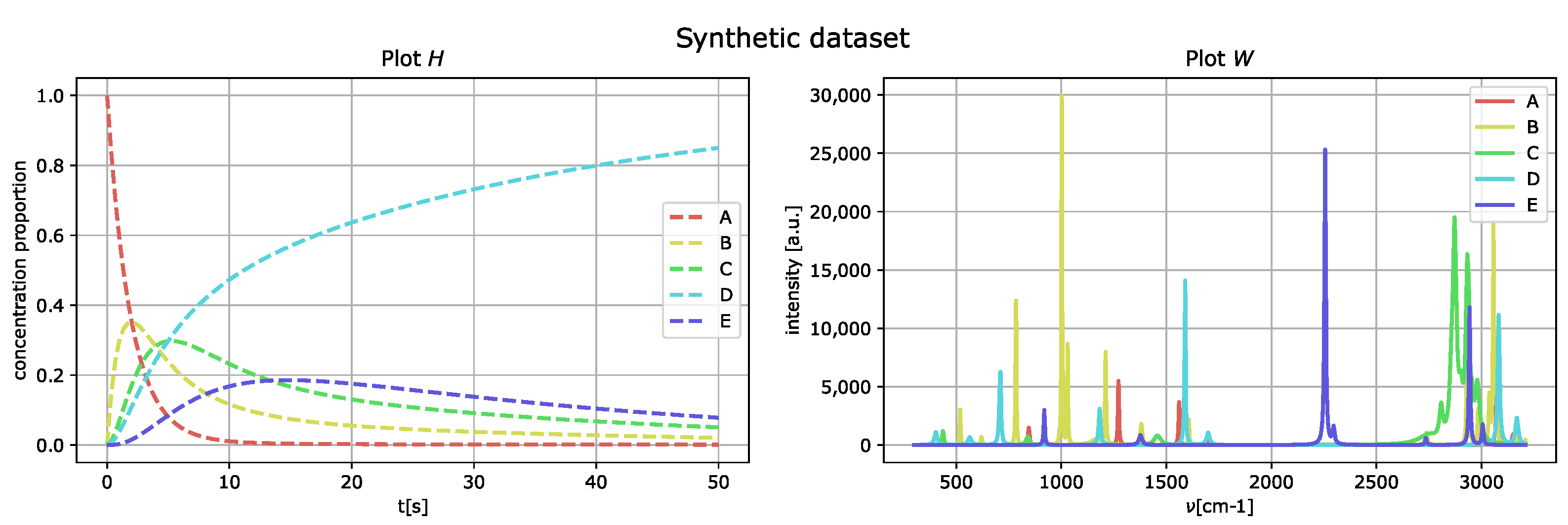
This first-order kinetics process describes the reaction of five compounds, called A, B, C, D, and E. The rate matrix Q that generates the kinetics is

$$\begin{array}{c}\hfill Q=\left(\begin{array}{ccccc}-0.53& 0.53& 0.00& 0.00& 0.00\\ 0.02& -0.66& 0.43& 0.21& 0.00\\ 0.00& 0.25& -0.36& 0.00& 0.11\\ 0.00& 0.00& 0.00& 0.00& 0.00\\ 0.00& 0.00& 0.10& 0.00& -0.10\end{array}\right).\end{array}$$

(13)

The concentration proportions of the chemical moieties evolve in time following the rule, $H{(t+\tau )}^T=H{\left(t\right)}^{T}exp\left(\tau Q\right)$.

The generated peak intensities consist of Lorentzian curves in the matrix W. The generated dataset is then given by

$$\begin{array}{c}\hfill M=WH,\end{array}$$

(14)

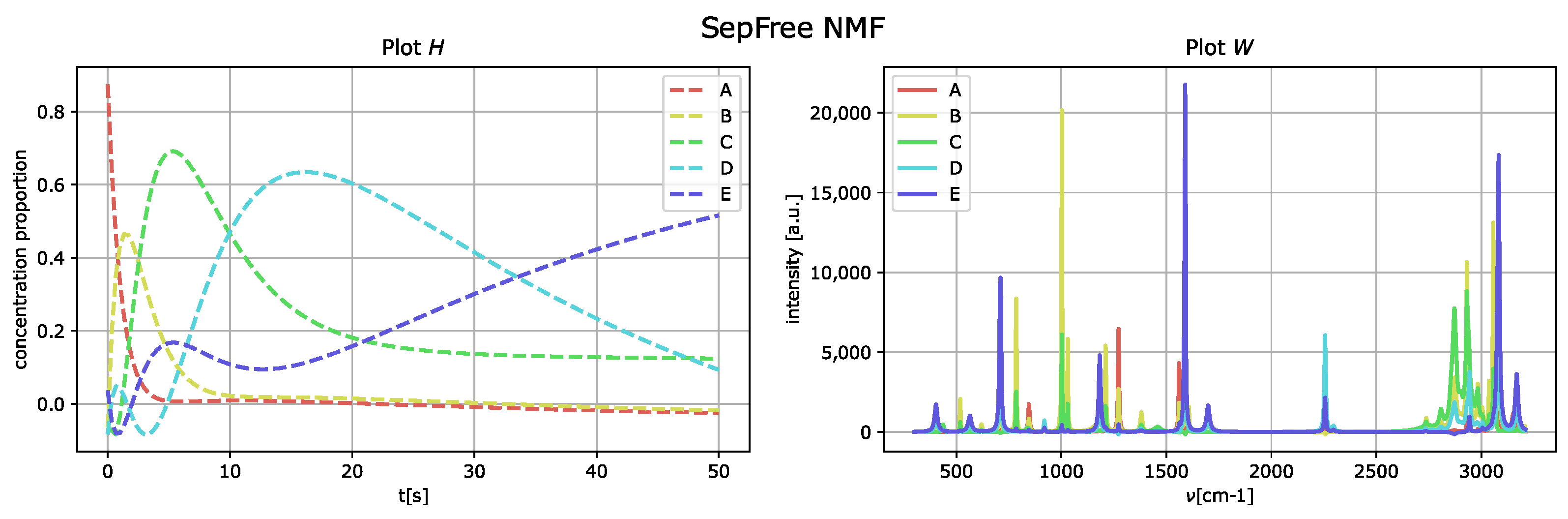
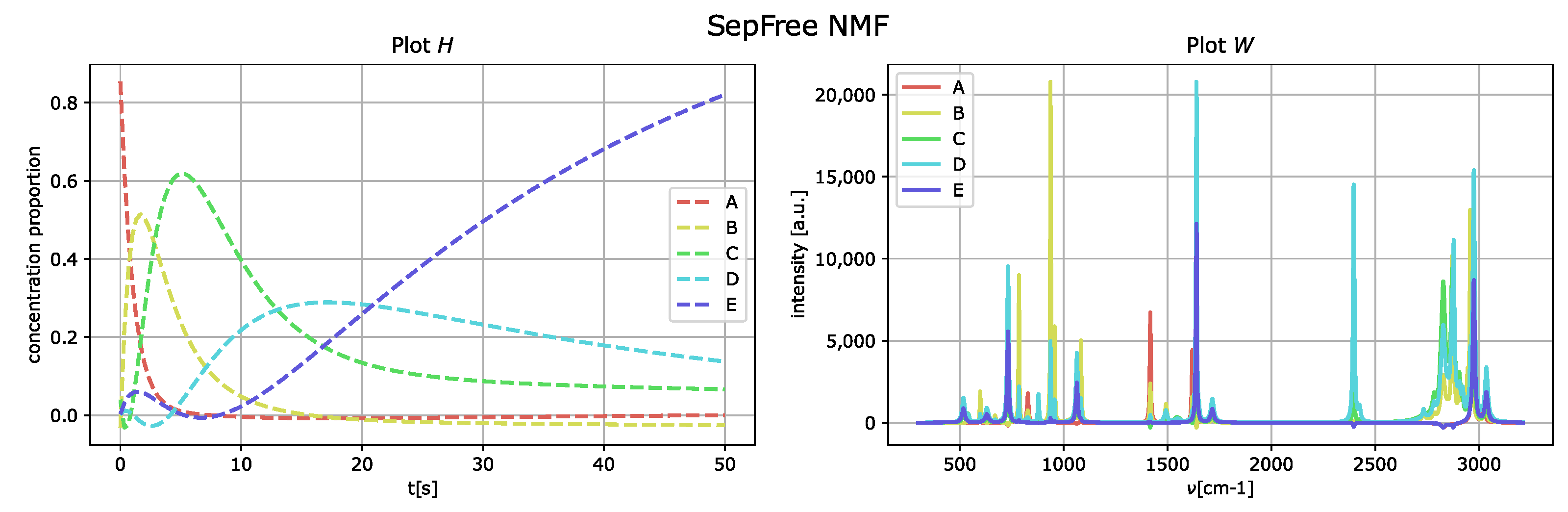
whereby no artificial noise is added, and the peaks of the matrix W are well separated. Figure 3 represents the generated spectral compounds as a function of the wavenumber $\nu$ (right) and their concentration proportions as a function of delay time t (left).

The outcome of the application of the algorithm in Section 2.1 is presented in Figure 4, and the parameters used for the optimization of the function $\mathsf{\Psi }$ are

$$\begin{array}{c}\hfill \alpha =-0.001,\beta =-10,\gamma =1,\delta =0,\mu =0.\end{array}$$

We set $\delta$ and $\mu$ to zero, since they are related to the computation of the Koopman transition probability matrix K. Thus, we do not need to bias the optimization of $\mathsf{\Psi }$ for K.

For determining the parameters for $\mathsf{\Psi }$, a heuristic method is used; see Appendix B.

By comparing the spectral fingerprint of species D and E, in Figure 4, to the spectral fingerprint of D of the generated dataset, Figure 3, we see that the species E obtained corresponds to the component labeled as D in Figure 3.

The memory effect for this reconstruction is $det\left(\mathcal{S}\right)=0.002$, which means that the memory effect for this decomposition is very strong. Additionally, the low value of the determinant is given by the fact that the reconstructed kinetic-matrix H contains some negative entries, even if they are close to zero.

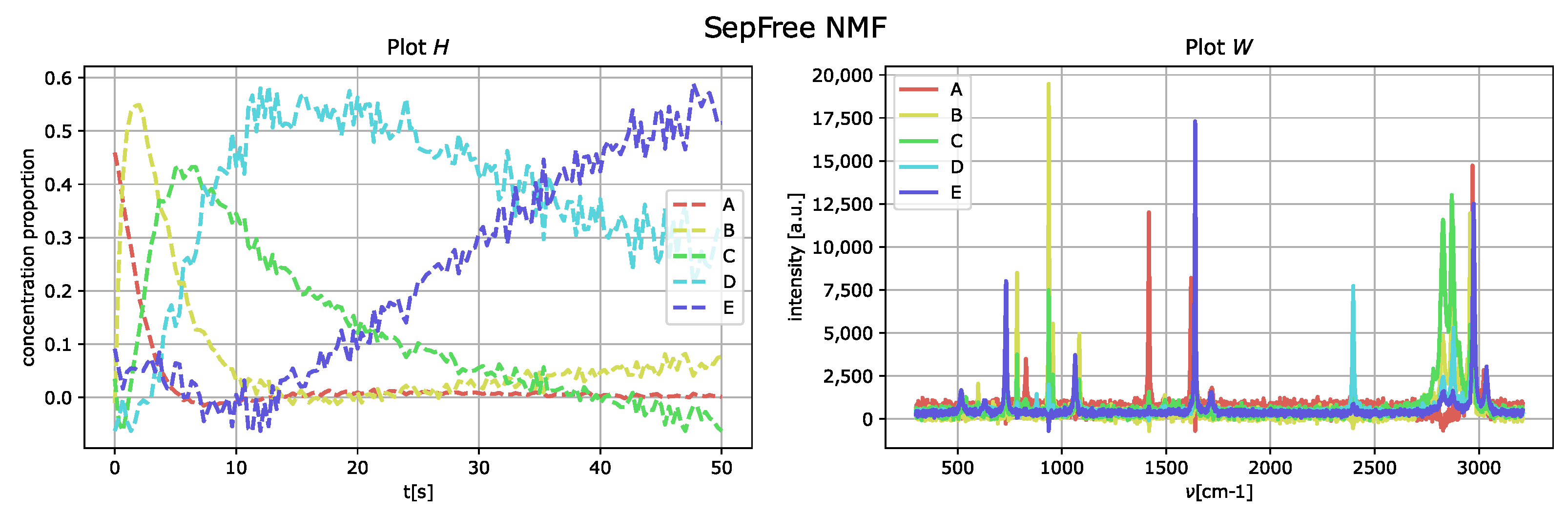
4.1.1. Synthetic Dataset with Increased Interference

To increase the interference level, the peaks of the matrix W are moved next to each other. The results of the analysis with SepFree NMF are displayed in Figure 5; the decomposition is computed for the same parameter set previously used. The minimal memory effect for increasing peak-interference of $30\%$ is $det\left(\mathcal{S}\right)=0.001$, so the memory effect becomes twice bigger by adding interference to the data.

As in the obtained results for the data without noise nor interference, the component E corresponds to the one labeled as D of the generated dataset.

4.1.2. Synthetic Dataset with Noise and Increased Interference

In order to consider the effects of the (experimental) noise to the analysis and for the computation of the minimal memory effect, the normally distributed noise matrix N, $N\in {\mathbb{R}}^{n\times m}$ is added to the data matrix M so that

$$\begin{array}{c}\hfill \tilde{M}=M+\eta N\end{array}$$

(15)

and the noise is scaled by a factor $\eta$, for this example $\eta =0.4$. The results of the decomposition are displayed in Figure 6. As in the obtained results for the data without noise nor interference, the component E corresponds to the species labeled as D of the generated dataset. The minimal memory effect computed with the decomposition is 0.0005. The introduction of the noise makes a remarkable difference in the memory properties of the spectrum. In comparison to the dataset with well-separated peaks and no additional noise, the minimal memory effect is four times bigger.

4.2. Raman Experiment-Crystallization of Paracetamol in Methanol

In this example, we show that the determinant of $\mathcal{S}$, defined in (12), is an effective measure for the physical meaningful number of compounds.

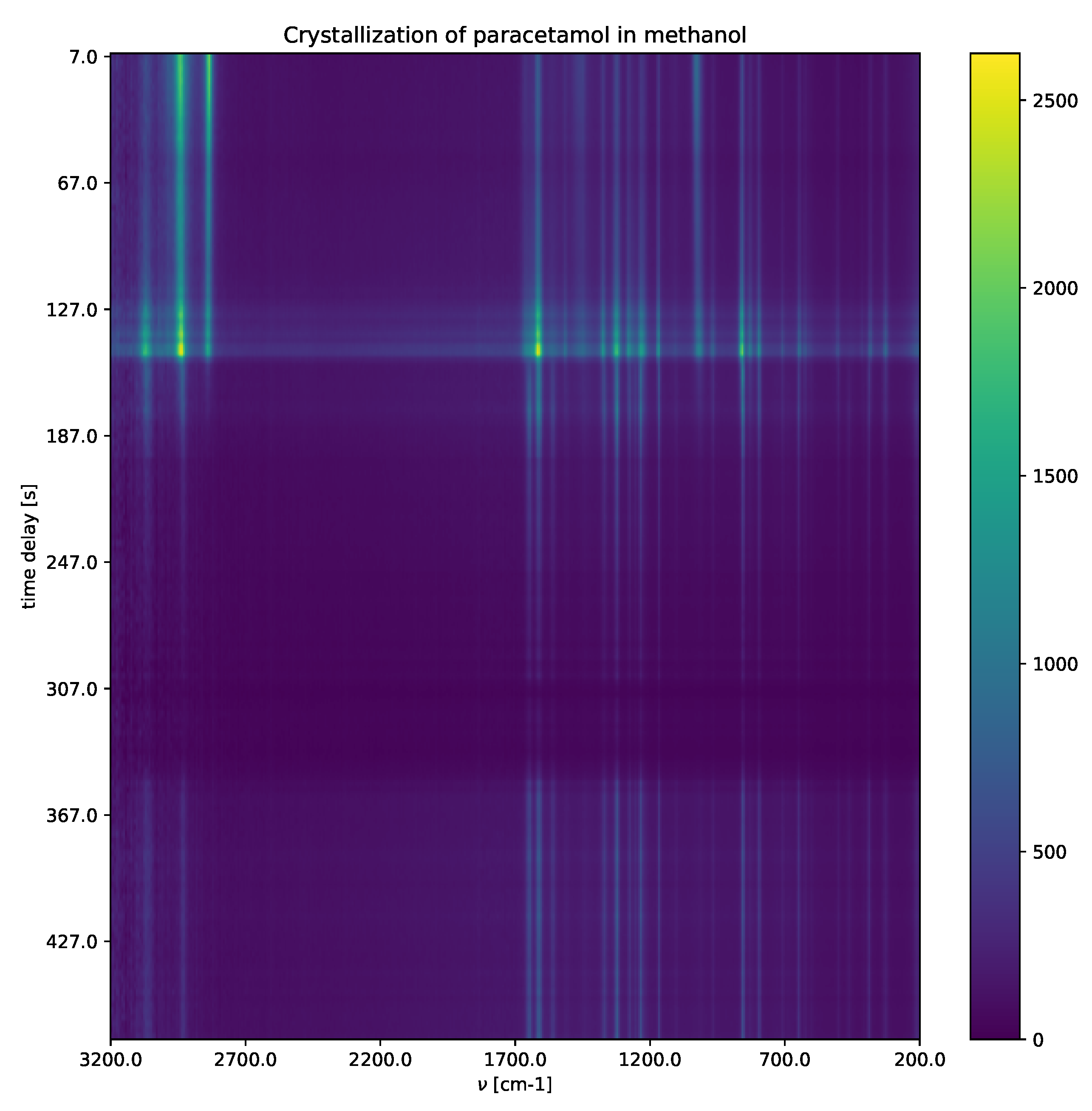
Crystallization of paracetamol in methanol (Figure 7) shows a solvated paracetamol in methanol, a metastable intermediate phase, and a crystalline phase. For detailed explanations, including the experimental settings, see Appendix A. Raman shifts characterize different paracetamol phases (solution phase, metastable intermediate phase and form II). After applying the SepFree NMF method, the role that the obtained compounds have in the reaction can be identified by the position of the peaks in matrix W.

Firstly, the singular value decomposition of the sequentially measured unprocessed spectral data taken as matrix suggests that the number of compounds can probably be $r=3,4,5$. Thus, SepFree NMF is tested then for these r values. The parameters used for the objective function are $\alpha =0.1$, $\beta =1000.0$, $\gamma =50.0$, $\delta =1.0$, $\mu =1.0$.

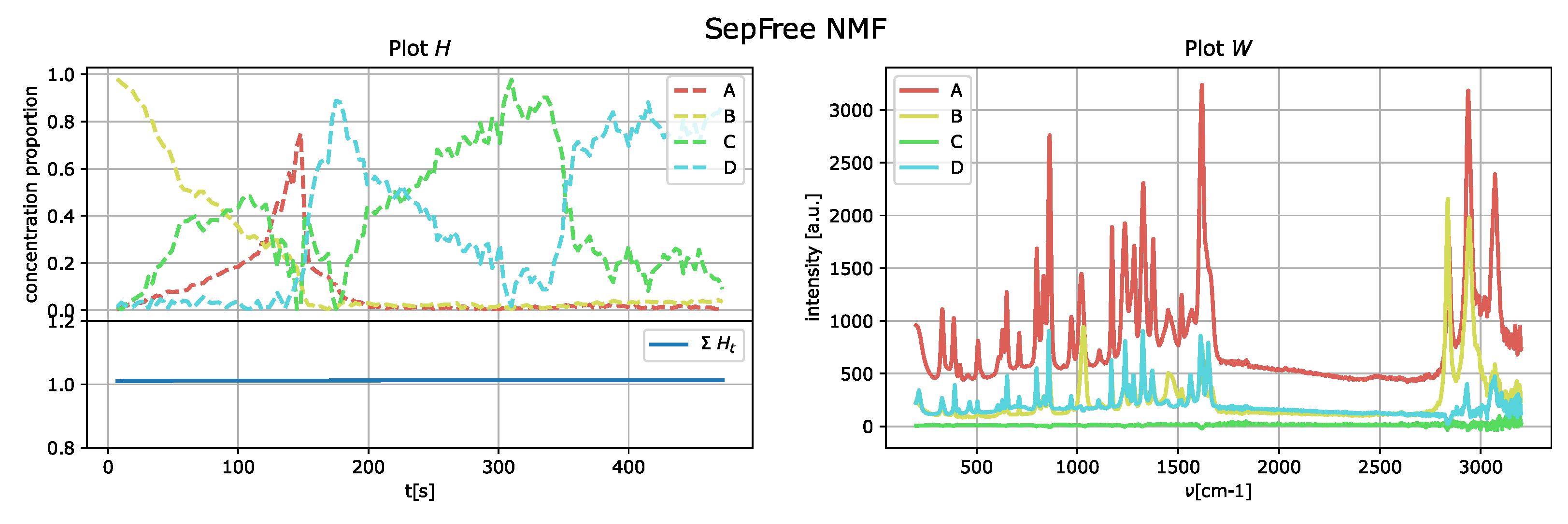
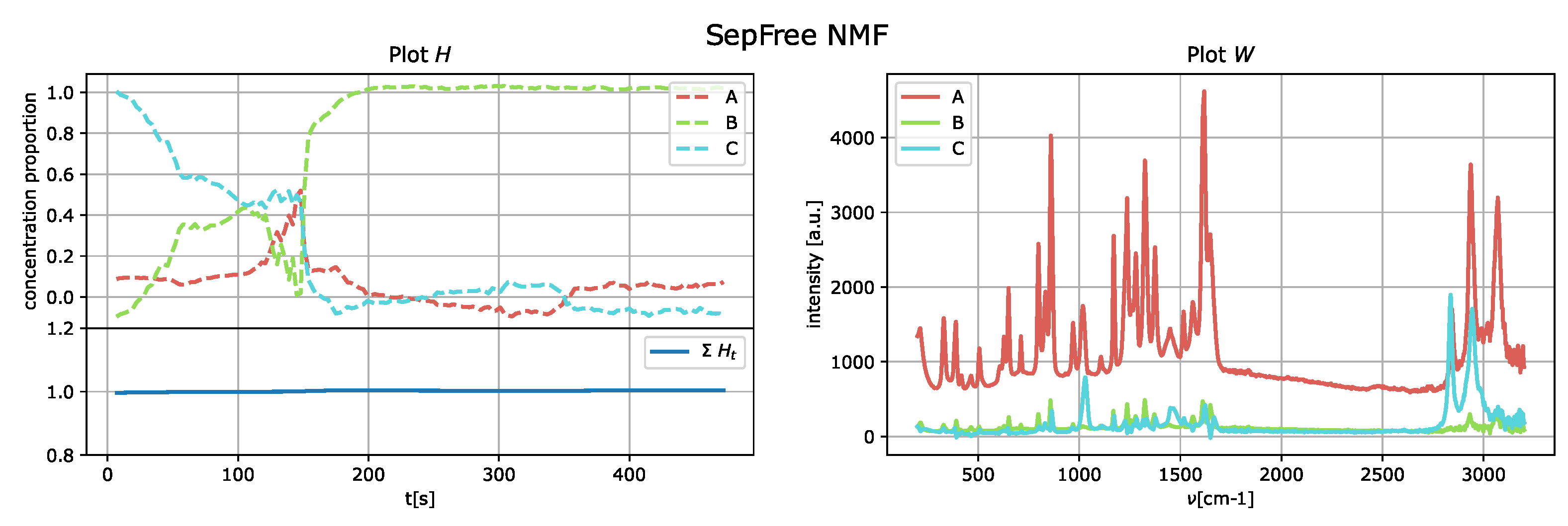
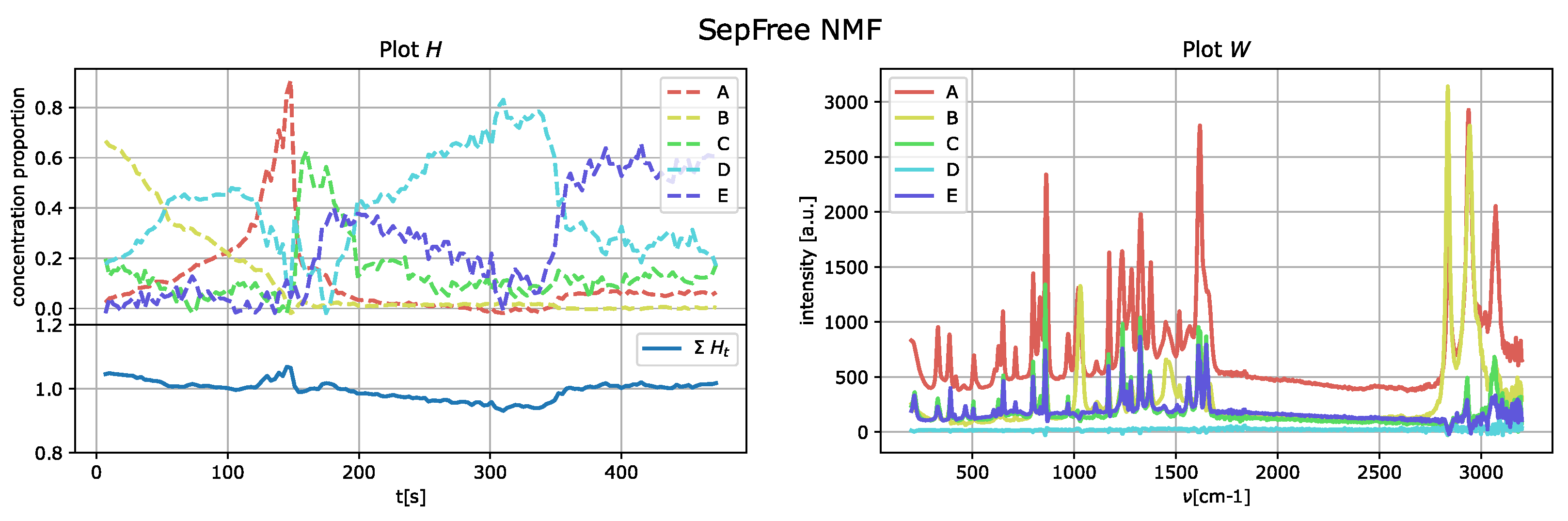
The results of the application of the SepFree NMF are shown in Figure 8 for $r=3$, in Figure 9 for $r=4$, and in Figure 10 for $r=5$. In each figure, the left plot shows the row of the matrix H as function of the delay time t; the right plot displays the peak intensities of W as function of the Raman shift (cm⁻¹). The sum of the relative concentrations $\sum H_t$ is also plotted on the left below, since the sum of the compounds can change. This change is due to variations of state occurring in the reaction, which modify the relative concentrations of the paracetamol moieties.

The decomposition with $r=4$ and $r=5$ compounds show kinetic curves in which the state’s proportion rises, decreases and rises again, as it can be seen in Figure 9 and Figure 10. This pattern cannot explain the state of a compound in a crystallization process. In contrast, the decomposition in Figure 8 for $r=3$ describes a sequential kinetic process, as expected for a crystallization.

Can we estimate the number of reaction compounds only by looking at $det\left(\mathcal{S}\right)$?

This question can be answered with yes by

Table 1. Number of compounds r in the decomposition and respective minimal memory effect, $det\left(\mathcal{S}\right)$. The decomposition with the smallest minimal memory effect is the one with $r=3$. The minimal memory effect for $r=4$ and $r=5$ is orders of magnitude greater.

r	$det\left(\mathcal{S}\right)$
3	0.106
4	0.031
5	0.001

. In this table, the values of $det\left(\mathcal{S}\right)$ for $r=3,4,5$ are given. It can be noticed that for $r=3$ the determinant has the highest value, in accordance with the above considerations on the kinetics.

The SepFree NMF yields also a transition matrix $K\left(\tau \right)$ for the process [6]. Examining the transition matrix allows to understand the kinetic model underlying the reaction mechanism [18]. The crystallization process of this dataset is a sequential process.

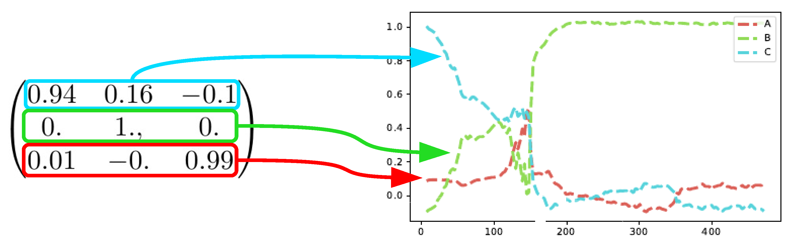
The matrix $K\left(\tau \right)$ resulting from the decomposition

$$\begin{array}{c}\hfill K\left(\tau \right)=\left(\begin{array}{ccc}0.94& 0.16& -0.1\\ 0.& 1.,& 0.\\ 0.01& -0.& 0.99\end{array}\right)\end{array}$$

(16)

shows also a sequential process $C\to A\to B$ and it shows that B is an absorbing state of the Markovian process. This means that when the process reaches B, it does not leave that condition anymore, as also shown in Figure 11. The first compound for the analysis of the matrix $K\left(\tau \right)$ is C since C is the most abundant at time $t=0$, see Figure 8.

In the supplementary materials, we provide a similar analysis for the decomposition of ranks 4 and 5, showing that the kinetic model described is not sequential.

Recognizing the chemical moieties from the Raman shifts is advantageous for validating the number of compounds estimated with the minimal memory effect, as shown in the following analysis. To show that the results given by the decomposition of rank 3 are indeed in agreement with the experiment, we plot each peak intensity of W (Figure 8) with the peaks of form II and metastable amorphous form II. The values of the Raman peaks are reported in the supplementary materials.

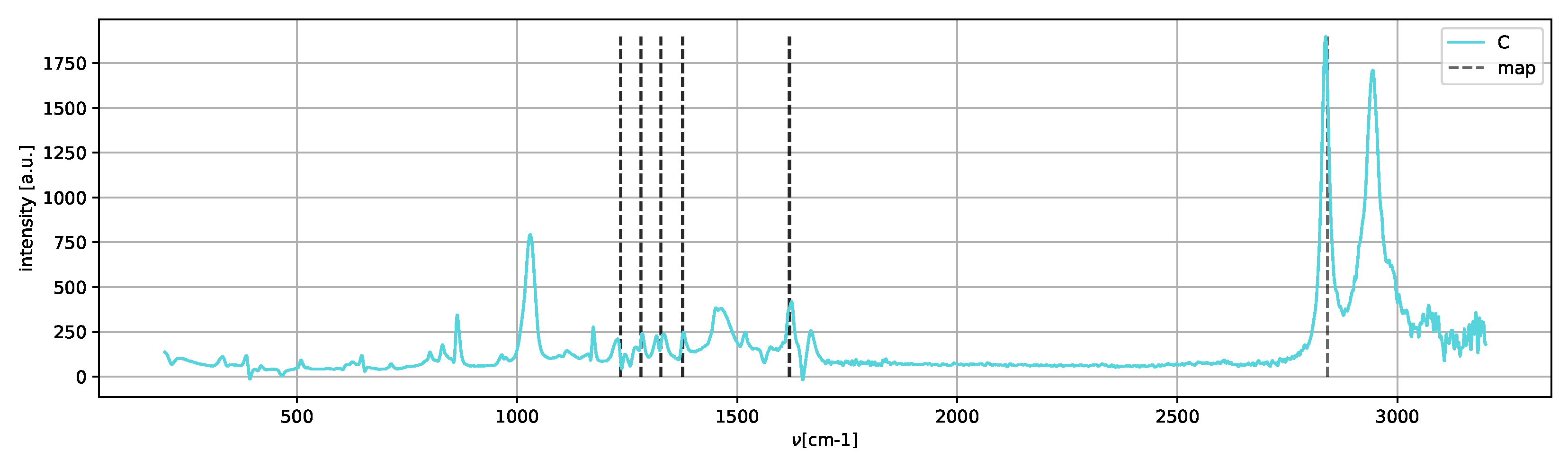
Spectrum C (Figure 12) shows only the peaks of the metastable amorphous phase and two clear peaks in the 2800–3000 cm${}^{-1}$ region, which can be assigned to methanol [25].

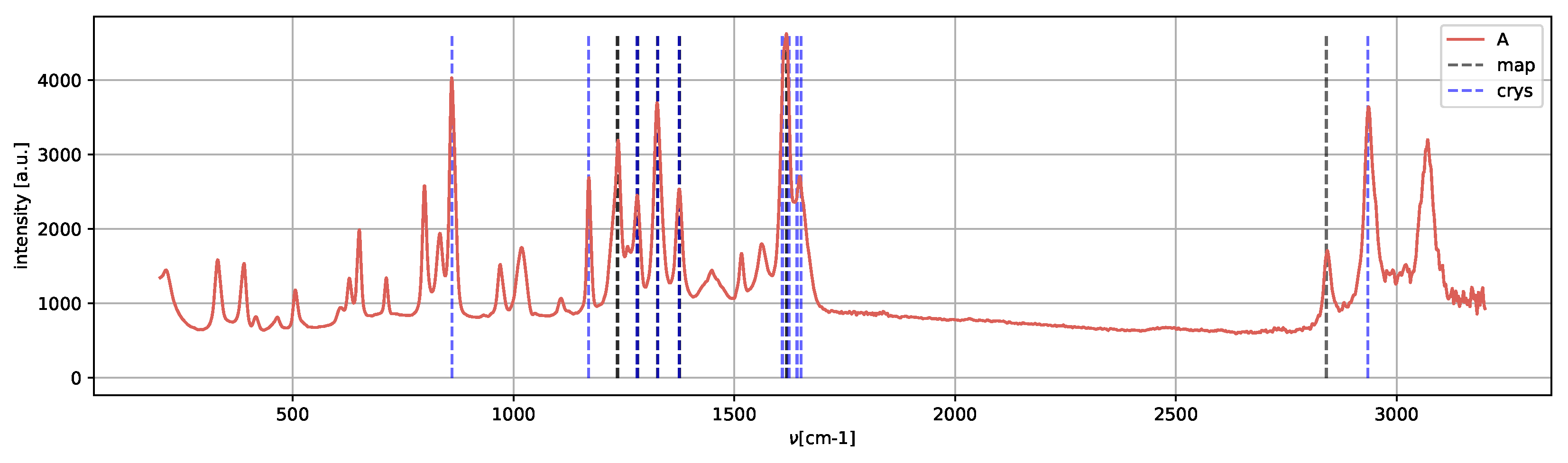
Spectrum A (Figure 13) presents the peaks characteristic of the metastable amorphous phase and solvent, as methanol Raman shifts are still present, in agreement with [25].

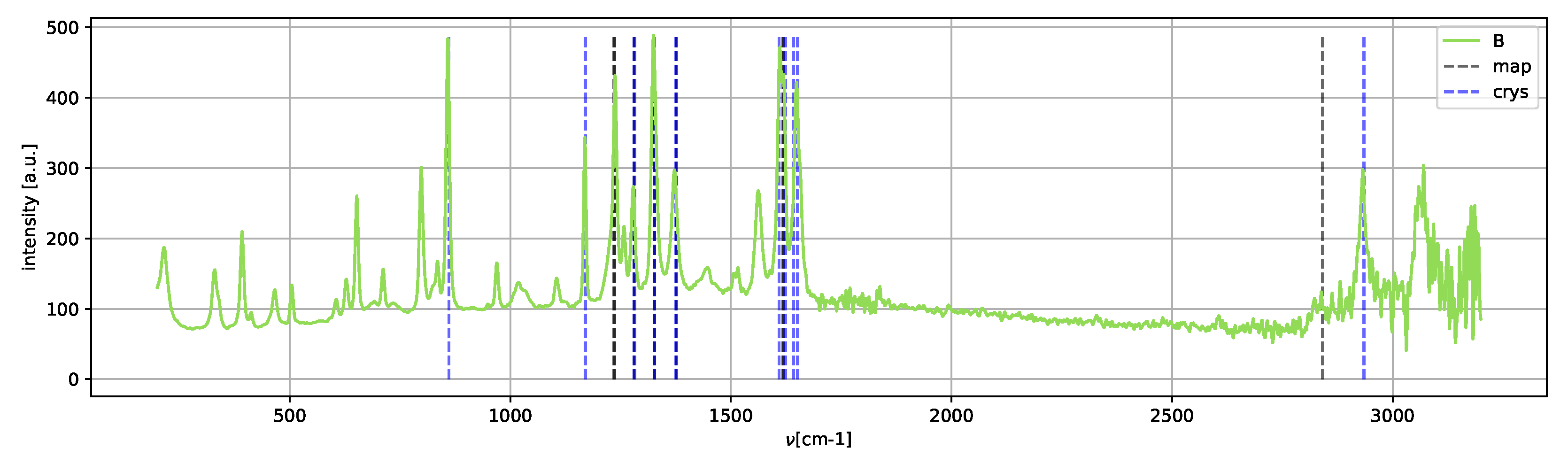
Spectrum B (Figure 14) shows the peaks of the crystallized form II; neither Raman shifts of the metastable amorphous phase nor methanol shifts are clearly present.

In conclusion, the decomposition analysis reveals three stages of the reaction:

• C: solution phase paracetamol (paracetamol + methanol);
• A: metastable amorphous phase and methanol;
• B: crystallized form II.

In this way, only by computing the minimal memory effect, we obtain a decomposition (a) that describes the correct kinetic process, (b) whose spectral intensities have a precise and clear interpretation.

5. Conclusions

SepFree NMF is a new method to process sequentially measured spectra and estimating the number of components. It is available as Python code using the link in the Data Availability Statement. This link includes a script for the presented figures as well as a tutorial to reproduce the results. Former methods extracting the kinetics of a molecular process observed in a sequential spectroscopic experiment need prior knowledge about the number of chemical moieties and/or their spectroscopic fingerprints. For some methods, the separability assumption has to apply, which in principle also means that the pure spectroscopic fingerprints of the compounds are to be found in the measured spectrum. SepFree NMF can be applied without this kind of prior knowledge.

SepFree NMF simultaneously generates the kinetic curves together with the spectroscopic fingerprints. How does it differ from other methods based on experimental data? On top of the measured data, it additionally uses the fact that the projected macro process is assumed to be Markovian. Thus, there should a transition matrix $K\left(\tau \right)$, and there should be as few memory effects as possible in the projection. We show that $det\left(\mathcal{S}\right)$ is a good indicator for the memory effect. This structural information is the conceptual basis for formulating an optimization problem.

Using SepFree NMF, it is possible to extract the kinetics together with the number of compounds of a crystallization process observed with Raman spectroscopy. This would not be possible with methods which rely on the separability assumption.