Article

Semi-Automatic Multiparametric MR Imaging Classification Using Novel Image Input Sequences and 3D Convolutional Neural Networks

1
Graduate School of Science and Technology, Chiba University, Chiba-shi 263-8522, Japan
2
Department of Urology, Toho University Sakura Medical Center, Sakura-shi 285-8741, Japan
3
School of Computer Science and Technology, Heilongjiang University, Harbin 150080, China
4
School of Medicine, Toyama University, Toyama 930-8555, Japan
5
Center for Frontier Medical Engineering, Chiba University, Chiba-shi 263-8522, Japan
*
Author to whom correspondence should be addressed.
Algorithms 2022, 15(7), 248; https://doi.org/10.3390/a15070248
Submission received: 21 May 2022 / Revised: 15 July 2022 / Accepted: 16 July 2022 / Published: 18 July 2022
(This article belongs to the Special Issue Algorithms for Biomedical Image Analysis and Processing)

Abstract

:
The role of multi-parametric magnetic resonance imaging (mp-MRI) is becoming increasingly important in the diagnosis of the clinical severity of prostate cancer (PCa). However, mp-MRI images usually contain several unaligned 3D sequences, such as DWI image sequences and T2-weighted image sequences, and there are many images among the entirety of 3D sequence images that do not contain cancerous tissue, which affects the accuracy of large-scale prostate cancer detection. Therefore, there is a great need for a method that uses accurate computer-aided detection of mp-MRI images and minimizes the influence of useless features. Our proposed PCa detection method is divided into three stages: (i) multimodal image alignment, (ii) automatic cropping of the sequence images to the entire prostate region, and, finally, (iii) combining multiple modal images of each patient into novel 3D sequences and using 3D convolutional neural networks to learn the newly composed 3D sequences with different modal alignments. We arrange the different modal methods to make the model fully learn the cancerous tissue features; then, we predict the clinical severity of PCa and generate a 3D cancer response map for the 3D sequence images from the last convolution layer of the network. The prediction results and 3D response map help to understand the features that the model focuses on during the process of 3D-CNN feature learning. We applied our method to Toho hospital prostate cancer patient data; the AUC (=0.85) results were significantly higher than those of other methods.

1. Introduction

Prostate cancer [1] is currently one of the deadliest cancers in men, with a very high incidence and death rate each year. According to the World Health Organization, in 2020, about 1.41 million people suffered from prostate cancer and 380,000 died from it [2]. Early diagnosis and treatment of prostate cancer can be highly effective in preventing the development of cancerous tissue and metastasis into advanced prostate cancer, effectively improving the five-year survival rate of prostate cancer patients and reducing patients’ suffering. The diagnosis of PCa is currently made clinically with a prostate-specific antigen (PSA) [3] blood test and digital rectal examination (DRE) [2], followed by a transrectal ultrasound (TRUS) biopsy if the PSA test result is positive. However, due to the limited number of biopsy samples and/or the low ultrasound resolution of TRUS [4], lesions may be missed or the Gleason score (GS) determined from the biopsy sample may differ in repeat biopsies and, sometimes, from the score determined by radical prostatectomy. Moreover, prostate cancer is classified as clinically severe or clinically non-severe based on the GS, which is currently ≤7 for clinically non-severe prostate cancer and ≥8 for clinically severe prostate cancer. According to recent studies [3,5], the diagnosis of prostate cancer using PSA and biopsy has low sensitivity and specificity, which can lead to underdiagnoses and overtreatment, thus causing unnecessary suffering to patients. According to a recent study [6], the positive predictive values of DRE, TRUS, mpMRI, and TPSA levels for PCa were 39.91%, 39.38%, 64.14%, and 41.57%, respectively; the sensitivity of these parameters was 37.35%, 51.41%, 74.69%, and 57.43%, respectively; the specificity of these parameters was 62.26%, 46.90%, 71.97%, and 45.82%, respectively. Recent studies have demonstrated that multi-parametric magnetic resonance imaging (mp-MRI) [7,8,9] can provide a simpler, non-invasive, and more accurate method of detecting prostate cancer. By combining images different MRI modalities, these previous studies showed that mp-MRI images have a higher detection rate and better sensitivity and specificity for prostate cancer; because of the non-invasive and highly detectable nature of MRI, more and more studies are focusing on the classification of the clinical severity of prostate cancer under multiple modalities [10]. However, it is very difficult to manually perform operations such as classification and judgment of mp-MRI because there is a large number of images for each patient, thus requiring much time and expertise on the part of the radiologist for judging and interpretation analysis. In addition, due to the subjectiveness of the radiologist, there will be low sensitivity and specificity in analyzing and judging the images [11], especially in the articulation of different regions of the prostate. Therefore, there is a need for a computer-assisted prostate cancer classification method that can reduce the time required to classify prostate cancer and improve the specificity and sensitivity of prostate cancer diagnosis. In recent studies [6,12,13,14,15,16,17,18,19,20,21], methods were developed for automatic prostate cancer detection, diagnosis, and classification. Currently, the prostate cancer diagnosis method consists of three main parts: first, data pre-processing (cropping the overall prostate image to the prostate region or specific cancer site region); second, inputting the pre-processed image into a deep learning network for feature learning to obtain a feature map of the prostate; finally, outputting the results of the cancer grade according to the voxels in the learned feature map. The first computer-aided diagnosis system for prostate cancer, which was designed by Chen et al. [22], extracts pixel features from T2-weighted images (T2) with a matrix and discrete cosine transform, and then uses an SVM classifier to classify the peripheral regions of the prostate. In addition, Langer et al. [23] classified the peripheral zone (PZ) of the prostate using a dynamic contrast-enhanced (DCE) map, and Tiwari et al. [24] designed a classification system using semi-supervised multi-modal data. However, these studies separated different regions of the prostate, causing cancer at the junction of different regions to be easily missed and global features of the prostate to be ignored. Many recent studies focused on improving neural network models, but it is known that deep learning is still almost a black-box [25] system, and the intermediate learning process is difficult to understand. Therefore, there is the field of explainable deep learning, including CAM (class activation mapping) [26] technology, which uses feature visualization to explore the working mechanisms of deep convolutional neural networks and the basis of judgment. However, when implementing CAM, it is necessary to change the structure of the network itself; thus, Grad-cam was investigated on the basis of CAM [27]. Grad-cam can be implemented without changing the structure of the network itself and can extract the heat map of features of any layer, and a recent study investigated Grad-cam++ [28] in order to optimize the results of Grad-cam and make the positioning more accurate.
In this paper, we design a novel method for prostate cancer classification based on fusing image features under multiple modalities to enable the classification of the clinical severity of prostate cancer with a single input rather than using a costly multiple-input method with complex training. Specifically, we align the T2 and DWI images of the same patient to align the prostate region in space, crop the whole MRI image to the prostate region, fuse the aligned images with the T2 and DWI images to form a new 3D image sequence (“sequence” is used in this article to refer to the “input sequence” of a neural network, not to refer to an MRI acquisition sequence), and then input the new 3D sequence into the 3D-CNN for feature learning. Finally, we output the features for prostate cancer severity classification and visualize the learning interest points of the network using the improved 3D-Grad-cam.
In this study, there are three main contributions:
(a)
We developed a novel 3D-CNN input method that maintains the advantage of a low training cost for a single input and the advantage of multi-modal feature fusion of previous multi-input models, such that the model can fully fuse multi-modal features and facilitate network prediction with a single input.
(b)
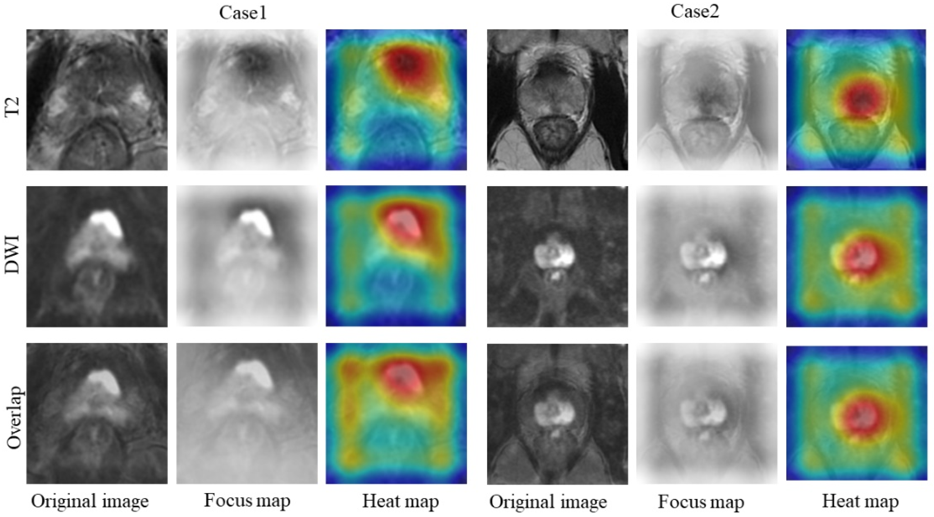
We improve the category activation map based on CAM by using the category activation map in a 3D image sequence to obtain a 3D-Grad-cam to facilitate our visualization of the network learning process.
(c)
We performed an extensive experimental evaluation and comparison and used different 3D-CNN models and different sampling methods for 3D-CNN models, and the AUC, sensitivity, and specificity of this method on a test dataset were 0.85, 0.88, and 0.88, respectively.
The rest of the paper is structured as follows. The following section focuses on the proposed method and the dataset used for the experiments, the Section 3 presents the experimental results and compares the baseline with the latest methods, the discussion is presented in the Section 4, and, finally, the conclusions are presented.

2. Methods

We predominantly used DWI and T2 image sequences from mp-MRI images in this study. Our main goal was to classify patients with prostate cancer as clinically severe and clinically less severe. Figure 1 illustrates the main framework of our proposed method, which has 3 main parts. First, we rigidly aligned [29,30] the T2 images with the DWI images in the planar spatial domain to correct the misalignment of the prostate region due to image sequences and biases with different MRI contrasts in the acquisition process. We then cropped out each T2 image with the DWI image containing the entire prostate region using an automatic method used for prostate region boundary detection, and then the cropped images were pixel-normalized. Third, we used the aligned and cropped T2 and DWI images to create a new 3D image sequence of the prostate, and we fed the new 3D image sequence into the 3D-CNN and obtained two outputs. The details of each step are presented in the following sections.

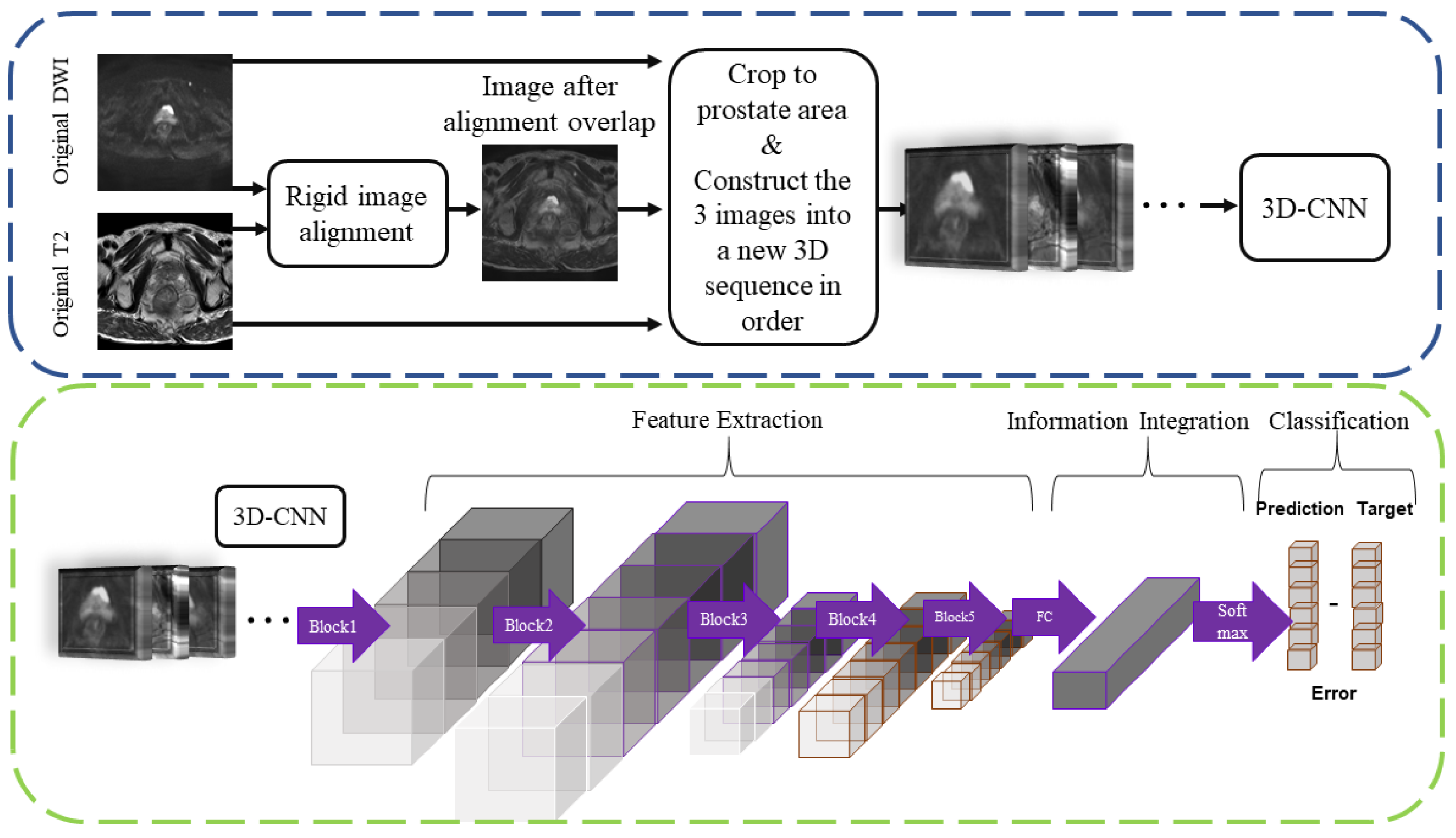
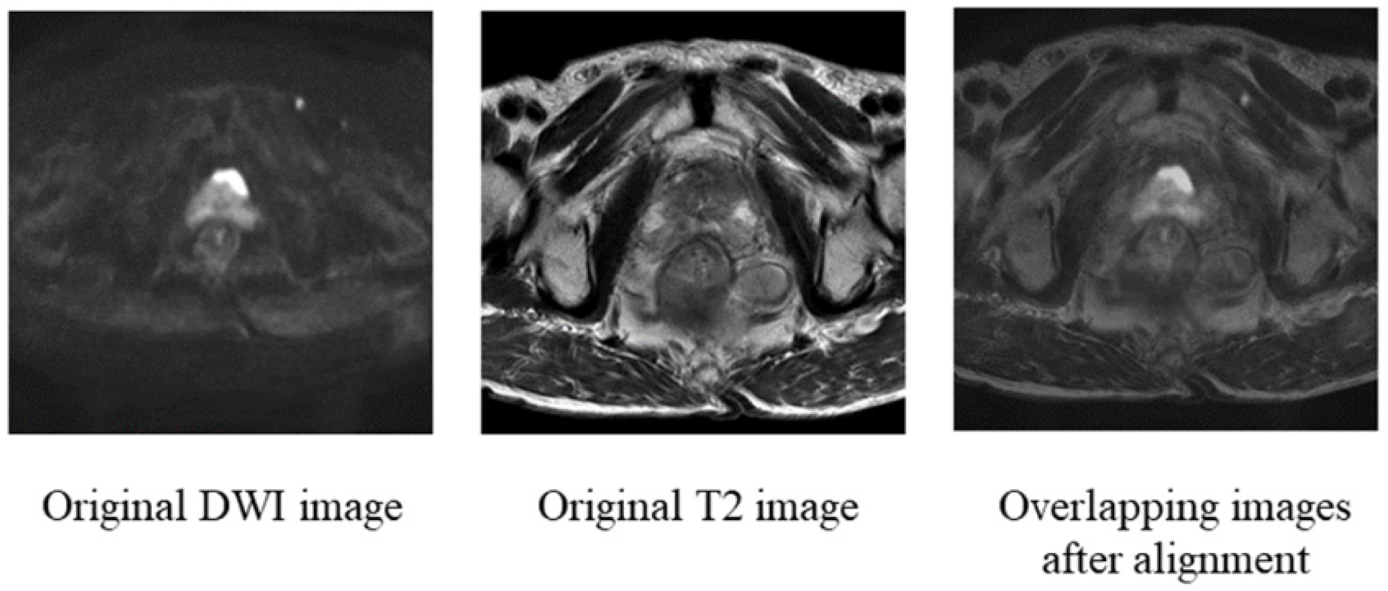
2.1. Rigid Alignment of DWI and T2 Images

In previous studies [6,8,13], it was demonstrated that, in prostate mp-MRI, different MRI sequences are deterministic for prostate cancer detection and classification results, but the sensitivity of detection results under single-modality images is limited, so there is a need to use multiple MRI sequences to make judgments and fully utilize the characteristics of cancerous tissues under different MRI contrasts. Among all mp-MRI sequences, T2 images are more favorable for prostate cancer detection and diagnosis based on previous studies, but the sensitivity of T2 images is low [4,31]. DWI images show the extent of water diffusion in the prostate due to the tight accumulation of cancer cells, and any changes in the prostate cancer can be detected more easily in DWI images; thus, DWI is another type of image recommended for use in diagnosis. However, DWI does not completely represent prostate lesions [31,32], so there are many studies combining DWI with T2 images to achieve better sensitivity and specificity [6,8,33]. As shown in Figure 2, in the present study, we use DWI and T2 sequences in mp-MRI for prostate cancer classification. One of the keys to accurately combining the DWI and T2 image features is to align the DWI and T2 sequences, which can effectively eliminate the small variations between different sequences caused by external factors during mp-MRI acquisition [11]. In this study, no drugs were used in the MR acquisition protocol to reduce and prevent motion. In order to ensure that the shape of the cancer lesion in the image is maintained without changing so that the model can acquire the actual features of the shape of the cancer lesion, we use a rigid 2D medical image alignment algorithm based on mutual information to maximize the mutual information between the reference image and the target image without changing the shape information of the cancerous region, and we use DWI as the target image and T2 as the reference image. In this study, we use DWI as the target image and T2 as the reference image. We use the best available medical image alignment algorithm, ANTs SyN [34], to align the images. The image alignment strategy generally starts with an initial globally aligned linear transformation, and the linear changes available in ANTs are optimized for the mean squared deviation and correlated similarity measures, each of which are optimized for translation and rotation. To ensure the accuracy of the alignment process, we checked each image after alignment.

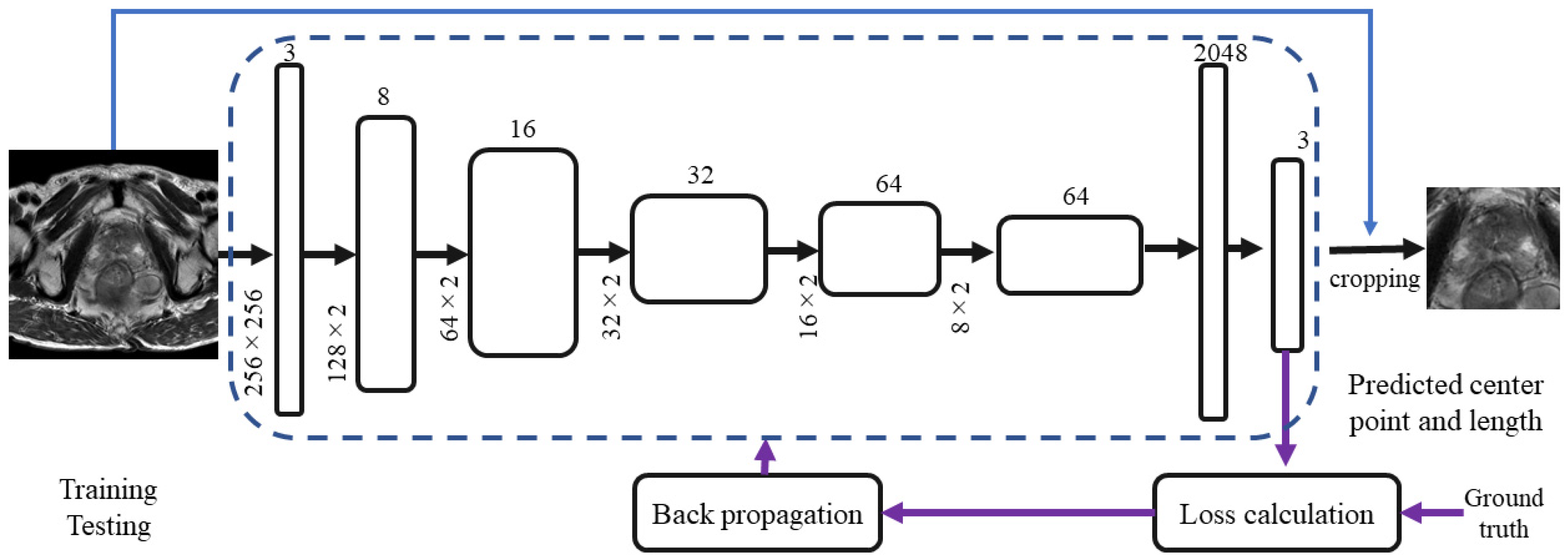
2.2. Prostate Area Cropping

After alignment, we used a basic regression CNN to crop each image into a square region containing the prostate region. Figure 3 shows the architecture of our CNN model for automatically cropping the prostate region. We took the original image for training; the bounding box of the prostate region was marked manually, and the model output three parameters: the center coordinates of the square region (x, y) and the length l. The activation functions of all layers were tan h functions, and the corresponding loss function of our model was:
l o s s = 1 / 3 ( | tan   h o 1 x t | + | tan   h o 2 y t | + | tan   h o 3 l t   | )
o 1 , o 2 are the x and y coordinates, respectively, and o 3 is the length. In the present study, though there have been more complex target detection networks, such as R-CNN [35] or automatic segmentation networks [36], in our experiments, a simple regression CNN was able to achieve the detection of the square prostate area more accurately, and the surrounding tissues outside the square prostate area did not have any effects on the detection of prostate cancer.

2.3. New Sequence-Based 3D-CNN

In the previous steps, we obtained the newly aligned DWI and T2 images. We arranged the aligned and cropped T2 and DWI prostate images and overlaid images in order to form a new 3D image sequence. In the next experiments, we resampled the new 3D image sequence of each patient 6 times (wince we used 3D convolution, the longer the z-axis of the input data was, the more z-axis features the model could learn, but considering that a longer input sequence for the model led to a significant increase in computation time and no significant improvement in the results, we chose to resample six times after the experiment); then, we input it into the 3D-CNN model to meet the training needs of the 3D-CNN model and obtained two outputs: (1) 3D class activation map, where the values of the pixels in the map represented the importance of having the model focus on this region; (2) high-dimensional semantic feature vectors, through which the 3D image sequence was classified.
There are three advantages to our use of this novel 3D-CNN input and training method: feature fusion, reinforcement features, and influence weight.
(1)
Feature fusion: With the 3D convolution kernel process and the operation of the spatial convolution of the image sequence, the convolution kernel will convolve the single image adjacent to the z-axis in the sequence image, and the features of the single image adjacent to the z-axis will be calculated by the convolution kernel and extracted as high-dimensional vectors. This operation is good for fusing all of the adjacent image features and can replace the traditional method with a multiple-input multi-MRI-contrast image method. We formed the images with different MRI contrasts into a new 3D image sequence so that neighboring images of each image in the sequence were images of various MRI contrasts. This method is a very cost-effective way to fuse image features with various MRI contrasts.
(2)
Reinforcement features: In building a new 3D image sequence, we built the images with several MRI contrasts in a different order to create a new image sequence; thus, the adjacent image MRI contrasts were often diverse, and the cancerous tissue features would be different in images with various MRI contrasts. The operation of the 3D convolution kernel caused the model to remember the features of cancerous tissue in the images with different MRI contrasts, which could enhance the learning of cancerous features.
(3)
Influence weight: In the learning of 3D convolution, the features of the image sequence were gradually high-dimensionalized, and the high-dimensional vector contained the full features of cancerous tissue; the linkage layer was expanded and the proportion of high-dimensional vectors containing cancerous tissue features to the total vectors increased, which could increase the accuracy of the prediction output. In the following, we provide detailed information on each step. In previous studies, the input of the 3D-CNN was usually a sequence of images of a patient with a particular MRI modality, but we fused images with different MRI contrasts into one sequence to be input into the network. The features of the image columns were extracted by the 3D-CNN, and the features of the z-axis were observable in the z-axis direction because each image of the new sequence had the most evident cancerous tissue. In Section 3, we use the best available 3D-CNN models for comparative experiments.

2.4. Implementations

All experiments in this study were conducted on a Windows computer using Python 3.6, with an Nvidia TITAN RTX graphics card and 24 GB of RAM, on an Intel(R) Core (TM) i7-9700K 3.60 GHz CPU. Pytorch [37] was used as the model backend to build the network architecture in all experiments. We used cross-entropy [38] as the loss function, trained for 2000 epochs with a batch size of 2, and the model converged at 500 epochs. We used Adam [39] as the model optimizer and set the learning rate to be automatically adjusted; the initial learning rate was 1 × 10⁻⁵, the learning rate was multiplied by 0.1 every 50 epochs, and the input images were flipped at a random level with a probability of 0.5 during training. The data were normalized, and all data were randomly divided into training, validation, and test sets with a ratio of 50:30:20; the input size of the model was 128 × 128, and network model was set to the model that preserved the best results.

3. Experiments

3.1. Setup

We collected T2 and DWI images of the prostate, which were used to train the model and evaluate the performance of the model.
The prostate MRI data used in this paper consisted of 129 samples from Toho University Medical Center, Japan (dataset A) and were acquired with 3T MR scanners (SIEMENS Skyra; syngo MR E11), as well as 121 samples from the 2017 SPIE-AAPM-NCI PROSTATEx challenge dataset (dataset B). The PROSTATEx Challenge [40] (“SPIE-AAPM-NCI Prostate MR Classification Challenge”) was held in conjunction with the 2017 SPIE Medical Imaging Symposium and focused on quantitative image analysis methods for diagnostic purposes and clinically meaningful prostate cancer classification. For each patient, the image with the most significant lesion area was selected.
The two datasets used—with data from different sites—were collected using different devices. We performed regularization preprocessing on these two datasets, as in the previous step. The method proposed in this paper was mainly used to predict high and low risk of early prostate cancer (according to the Gleason score, a score greater than or equal to 8 is considered clinically severe, and a score less than or equal to 7 is considered clinically insignificant). We used three main evaluation criteria to assess the performance of the model: the AUC (area under curve) value, sensitivity, and specificity, with the AUC being defined as the area under the ROC curve. Sensitivity (Se), called the true-positive fraction (TPF; or true-positive rate (TPR)), is the probability that a diagnostic test is correctly diagnosed as positive in a case group. Specificity (Sp), called the true-negative rate (TNF; or true-negative rate (TNR)), is the probability that the diagnostic test is correctly diagnosed as negative in the control group, and the false-negative rate (FNR; or false-negative fraction, FNF) is the probability that the diagnostic test is negative in the case group, which will lead to delayed disease and treatment. The false-positive fraction (FPF; or false positive rate (FPR)) is the probability that a diagnostic test is incorrectly diagnosed as positive in the control group. A false positive will result in incorrect treatment, and patients sometimes suffer from risky confirmatory tests.
sensitivity = TP TP + FN
specificity = TN FP + TN
In the above equation, TP, TN, FP, and FN represent the true positive, true negative, false positive, and false negative, respectively.
In the following sections, experiments are conducted to evaluate the performance of the proposed method in this paper. Table 1 shows the comparison experiments for the different 3D-CNN models, Table 2 shows the comparison experiments for the different newly ordered input sequences, and Table 3 shows the comparison experiments for the different modalities of the original image sequence; a comparison with the 3 latest methods is shown in Table 4.

3.2. Comparison with the Classic 3D CNN

In the first step of the experiment, we input the new 3D image sequences into different 3D-CNN models and uniformly used the pre-training weights of ucf-101 [41]. Table 1 shows the results of all of the 3D-CNN models when processing the new standard sequence images. All of the models were from [42]. From the comparisons, we found that, although the model parameters of ShuffNet were very limited, ResNet50 achieved the best AUC value in the test set. The sensitivity, specificity, and AUC values reached 0.88, 0.88, and 0.85, respectively.

3.3. Comparison of Different Input Orders

In the second step of the experiment, we input the images obtained in the previous steps into the model in different orders. In the previous step of the experiment (Section 3.2), the order of the single modal images in our new input image sequence was DWI, T2, and then overlaps. To find the most appropriate image alignment order for the input sequence, in this section, we divided the order in the new image sequence into four different orders:
(1)
Order one: DWI, T2, and then overlap as a set of re-sampling six times;
(2)
Order two: T2 re-sampling six times, DWI re-sampling six times, and then overlap re-sampling six times;
(3)
Order three: DWI re-sampling six times, T2 re-sampling six times, and then overlap re-sampling six times;
(4)
Order four: overlap re-sampling six times, T2 re-sampling six times, and then DWI re-sampling six times.
In the experiment in Section 3.2, 3DResNet50 achieved the best performance; we input different input sequences into the 3DResNet50 network, and in Table 2, we can see that the best results were produced by order 1.

3.4. Comparison Experiments with the Original 3D Sequence

In our study, we propose a new 3D-CNN sequence. In the experiment in this section, we compared this new sequence with the original image sequence (Table 3). We selected the integral unprocessed image sequence of each patient (T2 followed by DWI), and then we cropped the original 512 × 512 size to 384 × 384 and 128 × 128, respectively, for the input. The processed images were fed into the 3DResnet50 CNN, and Table 3 shows that the input of the original complete image sequence was not as good as the results of our proposed method.

3.5. Comparison with State-of-the-Art Methodologies

We also compared our proposed method with state-of-the-art methods, including the one proposed by Aldoj et al. [43] in 2020 for prostate cancer classification using multi-channel CNNs on multi-modal MRI images. Their method takes images of three modalities—ADC, DWI, and T2—as input, and inputs each modality into a different channel. There are 11 layers of 3D convolution with a convolution kernel of 3 × 3 × 3, an ensemble step of 2 × 2 × 2, and two fully connected layers. Because the method chooses data of three modes in the experiment, we only chose the results of two modes from Aldoj et al. [43] as input in order to balance the comparison of the experimental results. We can see that the sensitivity, specificity, and AUC values of our method were 0.14, 0.18, and 0.07 higher than those of the same two-modality image inputs, respectively. A recent study by Zhong et al. [44] used deep migration learning for prostate cancer classification based on multi-modal MRI images. It proposed feeding both T2 and ADC modality images into a deep migratory learning network for feature extraction and obtaining the prediction results after a fully connected layer. In the comparison experiments of Zhong et al. [44], they compared results using uni-modal and bi-modal image inputs. Here, for objectivity in the comparison experiments, we only selected the results of their comparison experiments with bi-modal inputs, and we found that the sensitivity, specificity, and AUC values of our model improved by 0.144, 0.08, and 0.127, respectively. Chen et al. [45] proposed an approach to classifying the clinical severity of prostate cancer using migration learning on the basis of multimodal MRI; the authors mainly used migration learning and pre-trained weights obtained after training on ImageNet, and they conducted their experiments using InseptionV3. The sensitivity, specificity, and AUC values of our method were 0.1, 0.05, and 0.002 higher than those of Chen et al. [45].

3.6. 3D-CNN Learning Process Visualization

There have been many previous studies [27,28] on deep learning model explanation and on deep learning visualization, among which the most well known is CAM. CAM shows the basis of its decision in the form of a heat map when a model is needed to explain the reason for its classification, such as when informing where there are focal points in the map. For a deep CNN, after multiple convolutions and pooling, the last convolutional layer contains the richest spatial and semantic information, and the next layers are the fully connected layer and softmax layer, which contain information that is difficult for humans to understand and display in a visual way. Therefore, in order to provide a reasonable explanation of the classification results of the convolutional neural network, it is necessary to make full use of the last convolutional layer, and CAM draws on the idea of the well-known paper on Network in Network [27], which uses GAP (global average pooling) to replace the fully connected layer. GAP can be considered as a special average pooling layer, except that its pool size is as large as the whole feature map, which is actually the average value of all pixels in each feature map. This greatly limits its use. If the model is already online or the training cost is very high, it is almost impossible to retrain it. The basic idea of Grad-cam is the same as that of CAM, which is to obtain the weights of each pair of feature maps and then find a weighted sum. CAM replaces the fully connected layers with GAP layers and retrains the weights, whereas Grad-cam takes a different approach and uses the global average of gradients to calculate the weights. Although Grad-cam and other similar methods are effective, they have limitations, such as the localization of multiple similar targets at the same time; even for a single object, Grad-cam cannot localize it completely. Based on Grad-cam, the authors of [28] proposed Grad-cam++, which improved the previous method, with the main contribution that ++ introduced a pixel-level weighting of the output gradient for a specific location. This method provides a measure of the importance of each pixel in the feature map, and more importantly, they derived closed-form solutions while obtaining exact higher-order representations, including softmax and exponential activation outputs. Our method requires one back-propagation, so the computational effort is consistent with the previous gradient-based method, but the results are more effective. It can be extended in the field of 3D deep learning visualization. In this paper, we used Grad-cam++ in a 3D image sequence, as shown in Figure 4; we found that the model accurately focused on the cancerous tissue by using the focus map and heat map, and it learned the feature details of the cancerous tissue.
Figure 4 shows the heat map obtained through 3D visualization, where the red area represents the area where the network model focused and learned features, and the area closest to the red indicates the area where the convolutional network focused more of its attention. From the figure, we can see that the areas on which the network model focused were the lesion areas.

4. Discussion

Few studies have used 3D-CNN to classify the clinical severity of prostate cancer. The main reason for this is that the cancerous tissue portion of a patient’s whole prostate sequence often accounts for only a small part of the entire prostate image sequence. Due to the very small size of the cancerous tissue, although 3D-CNN can learn the features of the sequence images better than 2D-CNN, it is also difficult to learn the features of the cancerous tissue adequately with very small targets, and it is easy for the large number of useless features in the prostate cancer image sequence to affect the model’s learning results. So, we proposed the method in this paper, which solves this problem perfectly, but it is difficult to determine an optimal sequence length when constructing a new image sequence; the original image sequence length is determined by the original sequence, but the newly constructed image sequence does not have a perfect graph column length. In this paper, we explored different alignment methods when constructing the sequence as much as possible, and in future experiments, the sequence length will be investigated in order to find an optimal sequence length. Although the method achieves great results in the direction of deep learning, it is not superior to the results of a simple semen test, so this method is one of the methods for assisting doctors in diagnosis. We carefully considered the issue of whether to use fully automatic segmentation of the prostate region when designing the method, and we also wish to automate the whole method as much as possible and to reduce the manual part as much as possible, so we will add this step to the CNN in future work to achieve full automation. However, in the current study, we also used some bounding boxes for manual animation, so the current method is still semi-automatic, and we will introduce automatic segmentation methods for medical images, such as U-net, into our method in future work.

5. Conclusions

In this paper, we proposed a novel method for constructing 3D-CNN sequences and used the newly constructed 3D image sequences as input for different 3D-CNN models in comparison experiments, compared the results after different fine-tuning based on the basic constructed method, and, finally, compared the results with those of other 3D-CNN methods. The results showed that our proposed method had the best AUC value of 0.85, and using the improved 3D model visualization method showed the focus of the model’s learning.

Author Contributions

Conceptualization, B.L.,T.N. and P.X.; Methodology, B.L.; Software, T.N.; Validation, B.L. and Y.Y.; Resources, R.O.; Data curation, R.O. All authors have read and agreed to the published version of the manuscript.

Funding

This research received no external funding.

Institutional Review Board Statement

Not applicable.

Informed Consent Statement

Not applicable.

Data Availability Statement

Not applicable.

Conflicts of Interest

The authors declare no conflict of interest.

References

  1. Mohler, J.; Bahnson, R.R.; Boston, B.; Busby, J.E.; D’Amico, A.; Eastham, J.A.; Enke, C.A.; George, D.; Horwitz, E.M.; Huben, R.P.; et al. Prostate cancer. J. Natl. Compr. Cancer Netw. 2010, 8, 162–200. [Google Scholar] [CrossRef] [PubMed]
  2. Gillessen, S.; Attard, G.; Beer, T.M.; Beltran, H.; Bjartell, A.; Bossi, A.; Briganti, A.; Bristow, R.G.; Chi, K.N.; Clarke, N.; et al. Management of patients with advanced prostate cancer: Report of the advanced prostate cancer consensus conference 2019. Eur. Urol. 2020, 77, 508–547. [Google Scholar] [CrossRef] [PubMed]
  3. Weinreb, J.C.; Barentsz, J.O.; Choyke, P.L.; Cornud, F.; Haider, M.A.; Macura, K.J.; Margolis, D.; Schnall, M.D.; Shtern, F.; Tempany, C.M.; et al. PI-RADS prostate imaging–reporting and data system: 2015, version 2. Eur. Urol. 2016, 69, 16–40. [Google Scholar] [CrossRef] [PubMed]
  4. Schröder, F.H.; Hugosson, J.; Roobol, M.J.; Tammela, T.L.; Ciatto, S.; Nelen, V.; Kwiatkowski, M.; Lujan, M.; Lilja, H.; Zappa, M.; et al. Screening and prostate-cancer mortality in a randomized European study. N. Engl. J. Med. 2009, 360, 1320–1328. [Google Scholar] [CrossRef] [Green Version]
  5. de Rooij, M.; Hamoen, E.H.; Fütterer, J.J.; Barentsz, J.O.; Rovers, M.M. Accuracy of multiparametric MRI for prostate cancer detection: A meta-analysis. Am. J. Roentgenol. 2014, 202, 343–351. [Google Scholar] [CrossRef] [PubMed]
  6. Bai, X.; Jiang, Y.; Zhang, X.; Wang, M.; Tian, J.; Mu, L.; Du, Y. The Value of Prostate-Specific Antigen-Related Indexes and Imaging Screening in the Diagnosis of Prostate Cancer. Cancer Manag. Res. 2020, 12, 6821–6826. [Google Scholar] [CrossRef]
  7. Fehr, D.; Veeraraghavan, H.; Wibmer, A.; Gondo, T.; Matsumoto, K.; Vargas, H.A.; Sala, E.; Hricak, H.; Deasy, J.O. Automatic classification of prostate cancer Gleason scores from multiparametric magnetic resonance images. Proc. Natl. Acad. Sci. USA 2015, 112, E6265–E6273. [Google Scholar] [CrossRef] [Green Version]
  8. Turkbey, B.; Choyke, P.L. Multiparametric MRI and prostate cancer diagnosis and risk stratification. Curr. Opin. Urol. 2012, 22, 310. [Google Scholar] [CrossRef]
  9. Peng, Y.; Jiang, Y.; Yang, C.; Brown, J.B.; Antic, T.; Sethi, I.; Schmid-Tannwald, C.; Giger, M.L.; Eggener, S.E.; Oto, A. Quantitative analysis of multiparametric prostate MR images: Differentiation between prostate cancer and normal tissue and correlation with Gleason score—a computer-aided diagnosis development study. Radiology 2013, 267, 787–796. [Google Scholar] [CrossRef]
  10. Turkbey, B.; Xu, S.; Kruecker, J.; Locklin, J.; Pang, Y.; Bernardo, M.; Merino, M.J.; Wood, B.J.; Choyke, P.L.; Pinto, P.A. Documenting the location of prostate biopsies with image fusion. BJU Int. 2011, 107, 53. [Google Scholar] [CrossRef] [Green Version]
  11. Valerio, M.; Donaldson, I.; Emberton, M.; Ehdaie, B.; Hadaschik, B.A.; Marks, L.S.; Mozer, P.; Rastinehad, A.R.; Ahmed, H.U. Detection of clinically significant prostate cancer using magnetic resonance imaging–ultrasound fusion targeted biopsy: A systematic review. Eur. Urol. 2015, 68, 8–19. [Google Scholar] [CrossRef] [PubMed]
  12. Liu, P.; Wang, S.; Turkbey, B.; Grant, K.; Pinto, P.; Choyke, P.; Wood, B.J.; Summers, R.M. A prostate cancer computer-aided diagnosis system using multimodal magnetic resonance imaging and targeted biopsy labels. Medical Imaging 2013: Computer-Aided Diagnosis. In Proceedings of the International Society for Optics and Photonics, Lake Buena Vista, FL, USA, 26 February 2013; Volume 8670, p. 86701G. [Google Scholar]
  13. Lemaitre, G. Computer-Aided Diagnosis for Prostate Cancer Using Multi-Parametric Magnetic Resonance Imaging. Ph.D. Thesis, Universitat de Girona, Escola Politècnica Superior, Girona, Spain, 2016. [Google Scholar]
  14. Litjens, G.J.; Vos, P.C.; Barentsz, J.O.; Karssemeijer, N.; Huisman, H.J. Automatic computer aided detection of abnormalities in multi-parametric prostate MRI. Medical Imaging 2011: Computer-Aided Diagnosis. In Proceedings of the International Society for Optics and Photonics, Lake Buena Vista, FL, USA, 4 March 2011; Volume 7963, p. 79630T. [Google Scholar]
  15. Litjens, G.J.; Barentsz, J.O.; Karssemeijer, N.; Huisman, H.J. Automated computer-aided detection of prostate cancer in MR images: From a whole-organ to a zone-based approach. In Proceedings of the Medical Imaging 2012: Computer-Aided Diagnosis, International Society for Optics and Photonics, San Diego, CA, USA, 23 February 2012; Volume 8315, p. 83150G. [Google Scholar]
  16. Artan, Y.; Haider, M.A.; Langer, D.L.; Van der Kwast, T.H.; Evans, A.J.; Yang, Y.; Wernick, M.N.; Trachtenberg, J.; Yetik, I.S. Prostate cancer localization with multispectral MRI using cost-sensitive support vector machines and conditional random fields. IEEE Trans. Image Process. 2010, 19, 2444–2455. [Google Scholar] [CrossRef] [PubMed]
  17. Niaf, E.; Rouvière, O.; Mège-Lechevallier, F.; Bratan, F.; Lartizien, C. Computer-aided diagnosis of prostate cancer in the peripheral zone using multiparametric MRI. Phys. Med. Biol. 2012, 57, 3833. [Google Scholar] [CrossRef] [PubMed]
  18. Tiwari, P.; Kurhanewicz, J.; Madabhushi, A. Multi-kernel graph embedding for detection, Gleason grading of prostate cancer via MRI/MRS. Med. Image Anal. 2013, 17, 219–235. [Google Scholar] [CrossRef] [Green Version]
  19. Wang, S.; Burtt, K.; Turkbey, B.; Choyke, P.; Summers, R.M. Computer aided-diagnosis of prostate cancer on multiparametric MRI: A technical review of current research. BioMed Res. Int. 2014, 2014, 789561. [Google Scholar] [CrossRef]
  20. Rundo, L.; Han, C.; Zhang, J.; Hataya, R.; Nagano, Y.; Militello, C.; Ferretti, C.; Nobile, M.S.; Tangherloni, A.; Gilardi, M.C.; et al. CNN-based Prostate Zonal Segmentation on T2-weighted MR Images: A Cross-dataset Study. In Neural Approaches to Dynamics of Signal Exchanges; Esposito, A., Faundez-Zanuy, M., Morabito, F., Pasero, E., Eds.; Springe: Singapore, 2020; Volume 151, pp. 269–280. [Google Scholar] [CrossRef] [Green Version]
  21. Rundo, L.; Han, C.; Nagano, Y.; Zhang, J.; Hataya, R.; Militello, C.; Tangherloni, A.; Nobile, M.S.; Ferretti, C.; Besozzi, D.; et al. USE-Net: Incorporating Squeeze-and-Excitation blocks into U-Net for prostate zonal segmentation of multi-institutional MRI datasets. Neurocomputing 2019, 365, 31–43. [Google Scholar] [CrossRef] [Green Version]
  22. Chan, I.; Wells, W., III; Mulkern, R.V.; Haker, S.; Zhang, J.; Zou, K.H.; Maier, S.E.; Tempany, C.M. Detection of prostate cancer by integration of line-scan diffusion, T2-mapping and T2-weighted magnetic resonance imaging; a multichannel statistical classifier. Med. Phys. 2003, 30, 2390–2398. [Google Scholar] [CrossRef]
  23. Langer, D.L.; Van der Kwast, T.H.; Evans, A.J.; Trachtenberg, J.; Wilson, B.C.; Haider, M.A. Prostate cancer detection with multi- parametric MRI: Logistic regression analysis of quantitative T2, diffusion-weighted imaging, and dynamic contrast-enhanced MRI. J. Magn. Reson. Imaging Off. J. Int. Soc. Magn. Reson. Med. 2009, 30, 327–334. [Google Scholar] [CrossRef]
  24. Tiwari, P.; Viswanath, S.; Kurhanewicz, J.; Sridhar, A.; Madabhushi, A. Multimodal wavelet embedding representation for data combination (MaWERiC): Integrating magnetic resonance imaging and spectroscopy for prostate cancer detection. NMR Biomed. 2012, 25, 607–619. [Google Scholar] [CrossRef] [Green Version]
  25. Castelvecchi, D. Can we open the black box of AI? Nat. News 2016, 538, 20. [Google Scholar] [CrossRef] [Green Version]
  26. Zhou, B.; Khosla, A.; Lapedriza, A.; Oliva, A.; Torralba, A. Learning deep features for discriminative localization. In Proceedings of the IEEE Conference on Computer Vision and Pattern Recognition, Las Vegas, NV, USA, 27–30 June 2016; pp. 2921–2929. [Google Scholar]
  27. Selvaraju, R.R.; Cogswell, M.; Das, A.; Vedantam, R.; Parikh, D.; Batra, D. Grad-cam: Visual explanations from deep networks via gradient-based localization. In Proceedings of the IEEE International Conference on Computer Vision, Venice, Italy, 22–29 October 2017; pp. 618–626. [Google Scholar]
  28. Chattopadhay, A.; Sarkar, A.; Howlader, P.; Balasubramanian, V.N. Grad-cam++: Generalized gradient-based visual explanations for deep convolutional networks. In Proceedings of the 2018 IEEE Winter Conference on Applications of Computer Vision (WACV), Lake Tahoe, NV, USA, 12–15 March 2018; pp. 839–847. [Google Scholar]
  29. Zitova, B.; Flusser, J. Image registration methods: A survey. Image Vis. Comput. 2003, 21, 977–1000. [Google Scholar] [CrossRef] [Green Version]
  30. Hill, D.L.; Batchelor, P.G.; Holden, M.; Hawkes, D.J. Medical image registration. Phys. Med. Biol. 2001, 46, R1. [Google Scholar] [CrossRef] [PubMed]
  31. Sankineni, S.; Osman, M.; Choyke, P.L. Functional MRI in prostate cancer detection. BioMed Res. Int. 2014, 2014, 590638. [Google Scholar] [CrossRef] [PubMed]
  32. Gibbs, P.; Tozer, D.J.; Liney, G.P.; Turnbull, L.W. Comparison of quantitative T2 mapping and diffusion-weighted imaging in the normal and pathologic prostate. Magn. Reson. Med. Off. J. Int. Soc. Magn. Reson. Med. 2001, 46, 1054–1058. [Google Scholar] [CrossRef] [PubMed] [Green Version]
  33. De Santi, B.; Salvi, M.; Giannini, V.; Meiburger, K.M.; Marzola, F.; Russo, F.; Bosco, M.; Molinariet, F. Comparison of Histogram-based Textural Features between Cancerous and Normal Prostatic Tissue in Multiparametric Magnetic Resonance Images. In Proceedings of the 2020 42nd Annual International Conference of the IEEE Engineering in Medicine & Biology Society (EMBC), Montreal, QC, Canada, 20–24 July 2020; pp. 1671–1674. [Google Scholar] [CrossRef]
  34. Avants, B.B.; Tustison, N.J.; Song, G.; Cook, P.A.; Klein, A.; Gee, J.C. A reproducible evaluation of ANTs similarity metric performance in brain image registration. Neuroimage 2011, 54, 2033–2044. [Google Scholar] [CrossRef] [PubMed] [Green Version]
  35. Girshick, R. Fast r-cnn. In Proceedings of the IEEE International Conference on Computer Vision, Santiago, Chile, 7–13 December 2015; pp. 1440–1448. [Google Scholar]
  36. Yu, L.; Yang, X.; Chen, H.; Qin, J.; Heng, P.A. Volumetric ConvNets with mixed residual connections for automated prostate segmentation from 3D MR images. In Proceedings of the Thirty-First AAAI Conference on Artificial Intelligence, San Francisco, CA, USA, 4–9 February 2017. [Google Scholar]
  37. Paszke, A.; Gross, S.; Massa, F.; Lerer, A.; Bradbury, J.; Chanan, G.; Killeen, T.; Lin, Z.; Gimelshein, N.; Antiga, L.; et al. Pytorch: An imperative style, high-performance deep learning library. Adv. Neural Inf. Process. Syst. 2019, 32, 8026–8037. [Google Scholar]
  38. De Boer, P.T.; Kroese, D.P.; Mannor, S.; Rubinstein, R.Y. A tutorial on the cross-entropy method. Ann. Oper. Res. 2005, 134, 19–67. [Google Scholar] [CrossRef]
  39. Kingma, D.P.; Ba, J. Adam: A method for stochastic optimization. arXiv 2014, arXiv:1412.6980 2014. [Google Scholar]
  40. Armato, S.G.; Huisman, H.; Drukker, K.; Hadjiiski, L.; Kirby, J.S.; Petrick, N.; Redmond, G.; Giger, M.L.; Cha, K.; Mamonov, A.; et al. PROSTATEx Challenges for computerized classification of prostate lesions from multiparametric magnetic resonance images. J. Med. Imaging 2018, 5, 044501. [Google Scholar] [CrossRef]
  41. Karpathy, A.; Toderici, G.; Shetty, S.; Leung, T.; Sukthankar, R.; Fei-Fei, L. Large-scale video classification with convolutional neural networks. In Proceedings of the IEEE conference on Computer Vision and Pattern Recognition, Columbus, OH, USA, 23–28 June 2014; pp. 1725–1732. [Google Scholar]
  42. Kopuklu, O.; Kose, N.; Gunduz, A.; Rigoll, G. Resource efficient 3d convolutional neural networks. In Proceedings of the IEEE/CVF International Conference on Computer Vision Workshops, Seoul, Korea, 27–28 October 2019; pp. 1910–1919. [Google Scholar]
  43. Aldoj, N.; Lukas, S.; Dewey, M.; Penzkofer, T. Semi-automatic classification of prostate cancer on multi-parametric MR imaging using a multi-channel 3D convolutional neural network. Eur. Radiol. 2020, 30, 1243–1253. [Google Scholar] [CrossRef]
  44. Zhong, X.; Cao, R.; Shakeri, S.; Scalzo, F.; Lee, Y.; Enzmann, D.R.; Wu, H.H.; Raman, S.S.; Sung, K. Deep transfer learning-based prostate cancer classification using 3 Tesla multi-parametric MRI. Abdom. Radiol. 2019, 44, 2030–2039. [Google Scholar] [CrossRef] [PubMed]
  45. Chen, Q.; Xu, X.; Hu, S.; Li, X.; Zou, Q.; Li, Y. A transfer learning approach for classification of clinical significant prostate cancers from mpMRI scans. Medical Imaging 2017: Computer-Aided Diagnosis. In Proceedings of the International Society for Optics and Photonics, Orlando, FL, USA, 16 March 2017; Volume 10134, p. 101344F. [Google Scholar]
Figure 1. The framework of the proposed method consists of four key steps: (1) rigid multiparameter (DWI, T2) image alignment, (2) prostate region cropping, and (3) building a new 3D image sequence for input into a 3D-CNN.
Algorithms 15 00248 g001
Figure 2. Examples of the alignment of DWI and T2 images are shown: (1) original T2 image, (2) original DWI image, and (3) aligned T2 image after being overlaid with the DWI image.
Algorithms 15 00248 g002
Figure 3. The figure shows the prostate detection and cropping procedure used in this paper. In the step of CNN-based prostate region detection, each rectangular box in the figure represents a feature map vector and shows the dimensional information of the feature map, the lower left corner of each feature map shows the length and width of the feature map, and the top shows the number of channels of the feature map. After this network, three output parameters can be obtained: the center coordinates (x, y) of the detected square region containing the prostate and the length of the square region L.
Algorithms 15 00248 g003
Figure 4. The 3D-CNN model was visualized for learning. The figure shows two cases; the first column of each case is the original image, the second column is the focus map obtained through calculation, and the third column is the heat map obtained through the 3D Grad-cam++ calculation.
Algorithms 15 00248 g004
Table 1. Comparison with 3D-CNN methodologies.
MethodsSensitivitySpecificityAUCCI 95%Parameters
C3D0.830.790.810.80–0.8378 M
3DSqueezeNet0.730.680.700.72–0.782.15 M
3DMobileNet0.740.670.690.73–0.758.22 M
3DShuffleNet0.740.650.680.74–0.766.64 M
ResNext1010.830.750.810.76–0.8248.34 M
3DResnet1010.880.880.830.84–0.8583.29 M
Our method + 3DResNet500.880.840.850.85–0.8744.24 M
Table 2. Comparison experiments with different sequence orders.
MethodsSensitivitySpecificityAUCCI 95%Parameters
Order 10.880.880.850.85–0.8744.24 M
Order 20.840.840.820.80–0.83-
Order 30.840.840.810.82–0.84-
Order 40.880.840.840.79–0.84-
Table 3. Comparison experiments of the original 3D sequence (input sizes were 384 × 384 and 128 × 128, respectively).
MethodsSensitivitySpecificityAUCCI 95%Parameters
T2(384)0.630.590.680.66–0.688-
T2(128)0.710.630.720.71–0.74-
DWI(384)0.610.540.710.69–0.72-
DWI(128)0.650.540.740.73–0.76-
Our method + 3DResnert500.880.880.850.85–0.8744.24 M
Table 4. Comparison with the three cited methods used to classify the clinical severity of prostate cancer.
MethodsSensitivitySpecificityAUCCI 95%Parameters
Zhong et al., 2019 [18]0.6360.800.7230.58–0.88--
Ajdoj et al., 2020 [19]0.740.700.78----
Chen et al., 2017 [17]0.780.830.83----
Our method0.880.880.850.85–0.8744.24 M
Publisher’s Note: MDPI stays neutral with regard to jurisdictional claims in published maps and institutional affiliations.

