On Edge Pruning of Communication Networks under an Age-of-Information Framework

Abstract

Effective non-repetitive routing among nodes in a network is an essential function in communication networks. To achieve that, pruning the links of the network is helpful with the trade-off of making the network less robust in transmitting messages while reducing redundancy to increase flow with limited network bandwidth, so we enhance the quality of service (QoS). In our paper, we study the case that if a link removal has either no effect or an insignificant effect on the Age of Information (AoI) of the messages delivered in the communication network. The pruning of such links can be applied to the k least significant links in terms of their impact on the AoI of the messages transmitted in the system. The objective of our work is to study the effect of pruning a number of links in a network on the AoI, in order to reduce the redundancy of the messages that may be received at the destination many times while transmitted only once. In our context, the objective of the communication system would be to maintain the information from the source as fresh as possible when it arrives at the destination while reducing the redundancy of messages. In this work, we introduce an efficient reduction method designed for series-parallel networks with links of exponentially distributed wait times. In addition, we consider the deterministic case and present the pruning technique when link removal would not affect the AoI. Lastly, we present a comprehensive simulation to study the effect of pruning the links on the AoI of the network and the redundancy of messages received by the destination.

1. Introduction

It is an important functionality in communication networks to achieve efficient non-repetitive routing among nodes. In our context, the objective of the communication system would be to maintain the information from the source as fresh as possible when it arrives at the destination while reducing the redundancy of messages. Ensuring that the average Age of Information (AoI) of such a system is small corresponds to maintaining the freshness of information about the status of the source at the destination.

The effect of removing nodes or links from a communication network is widely studied [1,2,3,4,5,6]. We can rank the significance of links depending on the effect of removing them from the network. An important application of doing that is to protect the most significant links of the network by deploying more resources there or enforcing specific policies in order to secure those most important links. This is the reason why some studies analyzed different link-removal strategies and their impact on many applications of communication networks that spawn different research areas [1,2,7,8,9,10,11,12,13,14]. On the other hand, we may utilize the ranking of the importance of the links in order to identify the least important link in the network, which will have the least effect in case of removing it, as we do in our work here.

Various criteria are adopted to determine the importance of links in communication networks. One of those criteria is the AoI which determines the freshness of the messages transmitted through the network. The new metric of AoI, which has spawned relevant performance metrics, has opened new research fields. In the context of timely updates, it is widely considered that those relevant performance metrics are desired to have values that guarantee some kind of high freshness of the information of the message when they arrive at the destination [15,16,17,18].

We investigate the two cases when a link removal either has no effect or insignificantly affects the AoI of the messages delivered in the network; we consider that link an insignificant link which we may prune. The pruning can be applied on the least k significant links in terms of their impact on the AoI of the messages transmitted in the system. In our model, we consider that each node forwards the messages toward the direction of the destination node once it receives the message.

The objective of our work is to study the effect of pruning a number of links in a network on the AoI in order to reduce the redundancy of the messages that may be received at the destination many times while transmitted only once. Thus, improving the quality of service (QoS). This duplicate of receiving the same messages would happen, for example, in general gossip networks [19].

Our results are summarized as follows:

• An efficient reduction method designed for series-parallel networks with links of exponentially distributed wait times or with links of deterministic periodic wait time.
• A pruning algorithm that determines the least significant link in the network, in terms of its effect on the AoI, and prunes it.
• A comprehensive simulation to study the effect of pruning the links on the AoI of the network and the redundancy of messages received by the destination.

The remainder of the paper is organized as follows. In Section 2, related work is reviewed. In Section 3, the general model of the problem is proposed. In Section 4, the network reduction method for our model is introduced. Section 5 discusses the characterization of the AoI under our model. Section 6 briefly visits the periodic case. Section 7 shows the simple pruning techniques. Section 8 presents the simulation results. Section 9 gives the conclusion.

2. Related Work

General simple multi-hop communication networks are widely studied [20,21,22]. For those networks, many routing schemes are designed in order to optimize over the minimum count of the hops for the message to get transferred or the minimum cost of the transmission through the links of the network [23]. Those metrics are not necessarily the best to consider. That is due to the fact that the new metric of AoI for the freshness of messages is recently used often to refer to as a good metric for the QoS of the network [24].

One of the simplest and most natural communication network models is the gossip network model which simply lets the nodes broadcast the messages that they receive to their neighbor set through the available directed links [19,20,21]. This model is different than the more typical method of routing that depends on choosing a path to route the message and evaluates the best possible route depending on the metric used, whether the metric is cost or time delay, or another metric. One of those standards is the best worst link in the path of the network. The best worst link is considered to be the link that is the most unreliable (in case of having unreliable links) over the path chosen by the routing scheme. This link is called the bottleneck link. Those routing schemes choose the path that has the best bottleneck link [19,21,22].

In contrast to the criterion of pruning in our work, the research in [25] considered the criterion of pruning to be the simplicity of the network by reducing the number of edges while introducing a trade-off between connectivity and simplicity. In addition, the approach introduced in [26] keeps important edges without losing connectivity by setting a criterion that depends on the best path function standard which assigns a different priority to each edge so that they can prune the edges with low priorities.

Other pruning methods were introduced before. For example, structural pruning was introduced in [27] which prunes subgraphs of the network while maintaining the hubs and brokers of the network. In addition, descriptive pruning in [27] basically assigns a specific attribute value to each node related to its connectivity and edge degree, and prunes the parts with lower attribute values. This is different than our work here in which we consider the expected AoI of the whole network as the metric for pruning.

In this work, we consider a transmission model similar to the gossip network model for transmitting messages by flooding the network, in which nodes broadcast the messages to their neighbors. This model has a huge drawback, which is the fact that the messages often are duplicated when they reach the destination node [19,23,24]. To the best of our knowledge, this is the first work that studies the effect of pruning the gossip network on the repetition of the messages and the AoI at the same time.

3. Proposed Model

In this section, we introduce the details of the network model we use in this paper as well as the AoI model that characterizes the freshness of the messages.

3.1. Series-Parallel Networks

In this work, we restrict our study to consider topologies of the network to be exclusively series-parallel topologies. Despite this restriction, the general approach can be applied to any topology. However, the network reduction that is studied later in this work can not be done unless it is a series-parallel network. This class of topologies arises naturally in many communication network applications [28]. Following we demonstrate briefly the definition of a series-parallel graph (graph means a general multigraph in this context) with the basic operations for constructing such graphs. The definition follows the convention of Eppstein in [29].

First, we need to name a more general class of graphs that is referred to as two-terminal graphs, which are any connected graphs with exactly two unique nodes called the source node s and the destination node d—that is, the simplest two-terminal graph is a pair of source-destination nodes linked through one edge.

The first graphs-composition operation is composition in parallel $C_p$ operation that performs on exactly two operands, a two-terminal graph $G_1$ and another two-terminal graph $G_2$. The composed graph $G_p=C_p(G_1,G_2)$ is another two-terminal graph that is the disjoint union of graphs $G_1$ and $G_2$ after unifying the source nodes of $G_1$ and $G_2$ to form the source node of $G_p$, and unifying the destination nodes of $G_1$ and $G_2$ to form the destination node of $G_p$ as well. Note that $C_p(G_1,G_2)=C_p(G_2,G_1)$. An example is demonstrated in Figure 1a.

The second graphs-composition operation is composition in series $C_s$ operation that performs on exactly two operands, a two-terminal graph $G_1$ and another two-terminal graph $G_2$. The composed graph $G_s=C_s(G_1,G_2)$ is another two-terminal graph that is the disjoint union of graphs $G_1$ and $G_2$ after unifying the destination node of $G_1$ with the source node of $G_2$. The source node of $G_s$ is the source node of $G_1$, and the destination node of $G_s$ is the destination node of $G_2$. Note that $C_s(G_1,G_2)\ne C_s(G_2,G_1)$. An example is demonstrated in Figure 1b.

Now, we have everything set up to define series-parallel graphs.

Definition 1.

A series-parallel (SP) graph is a two-terminal graph that may be assembled from a set of connected pairs of nodes (source and destination nodes) with one edge using a specific order of the $C_p$ and $C_s$ operations.

It is worth mentioning that all the nodes in an SP graph that are not the source node or the destination node must have a degree of at least 2. Furthermore, the SP graph is always a planar graph. Figure 1c shows an example of the SP graph. For the sake of simplicity, we will represent $C_s(G_1,G_2)$ by $[G_1,G_2]$, and $C_p(G_1,G_2)$ by $[G_1\parallel G_2]$.

3.2. Age of Information

In this subsection, we briefly visit the standard definition of AoI used in this work, which is the metric used to measure the freshness of messages.

Consider a source-destination network. Now, consider $t_k$ to be the times at which the source node s receives a message. Let $t_k^{\prime }$ be the times at which this message is received by the destination node d. We then introduce the indexing function that takes t as an input and gives the index of the most recently received message at the destination node d. So that, the indexing function $N\left(t\right)$ is shown as follows:

$$N\left(t\right)=max\left\{k\right|t_k^{\prime }\le t\}$$

(1)

To this end, we have everything set up to define the standard AoI of any message at time t. The AoI that a system has which depends on the generation and receiving time of messages is given as follows [30]:

$$\Delta \left(t\right)=t-t_{N\left(t\right)}$$

(2)

In Figure 2, we see the basic representation of the AoI model that we use as the metric of message freshness. From now on in the paper, when we mention the AoI, we refer to the average AoI value that can be evaluated depending on the distribution of the generation times and delay of the network.

In this work, we consider the case at which the time taken for a link (indexed i) to be activated, in order to transfer the message awaiting at one of its nodes, to follow the exponential distribution where the average time taken for activation is $\frac{1}{{\lambda }_i}$ units of times counted from the moment the message arrives at one of its nodes. For now, we study the case where the time taken for the message to be transferred through the link is always insignificant compared to the average wait time $\frac{1}{{\lambda }_i}$. The activation times of the links are modeled as independent random variables.

3.3. Phase-Type Distribution

In this subsection, we introduce the Phase-type distribution. A phase-type distribution is a probability distribution that we may construct by a mixture of independent exponential distributions. It arises out in a natural way from a setting of sequence inter-related Poisson processes. One of the standard applications in which Phase-type distribution appears is when we model a representative random variable related to a Markov chain with one absorbing state. This random variable describes the total elapsed time until absorption. Each one of the states in the Markov process is represented by one phase [31].

Furthermore, an important characteristic of phase-type distributions is that they are dense on the field of analytical probability distributions. This means that this distribution closely approximates all positive-valued analytical distributions. It is worth mentioning that in our context here, we make use of a continuous-time Markov process with exactly $m+1$ states. All states are transient states except state 0. State 0 is the sole absorbing state of the Markov process.

To start defining the parameters of the distribution, consider that the Markov process has an initial probability distribution to start at any one of the different $m+1$ phases. This distribution of probabilities can be represented as the vector $({\alpha }_0,\mathit{\alpha })$ such that $\mathit{\alpha }$ is a $1\times m$ vector. From there, The phase-type distribution is used for a random variable that represents the time elapsed from the starting of such a process until the end, i.e., the absorption state 0.

To this end, The transition rate matrix of the Markov process is:

$$Q=\left[\begin{array}{cc}0& \mathbf{0}\\ {\mathbf{S}}^0& \mathbf{S}\end{array}\right]$$

(3)

such that the size of $\mathbf{S}$ is $m\times m$, and that $S^0=\mathbf{S}\times \mathbf{1}$, where $\mathbf{1}$ is the $m\times 1$ vector of unity elements.

Now, we define the random variable Z which has the probability distribution of the elapsed time the Markov process takes until absorption. The phase-type distributed to this end is typically denoted as $PH(\mathit{\alpha },\mathbf{S})$ [32].

The cumulative distribution function (CDF) of the random variable Z is given by $F\left(z\right)=1-\mathit{\alpha }exp\left(Sz\right)\mathbf{1}$. The probability density function is given by $f\left(z\right)=\mathit{\alpha }exp\left(Sz\right){\mathbf{S}}^{\mathbf{0}}$ for all $x>0$, where exp(·) is the matrix exponential operation. This operation is defined as $exp\left(\mathit{X}\right)={\Sigma }_{k=0}^{\infty }\frac{1}{k!}{\mathit{X}}^k$.

Typically, the trivial case of starting at the absorption state is discarded by setting the probability of starting there to zero (setting ${\alpha }_0=0$). Furthermore, We may derive the moments of the distribution by $E\left[X^n\right]={(-1)}^{n}n!\mathit{\alpha }{S}^{-n}\mathbf{1}$. The Laplace transform of the distribution can be derived as well by $M\left(s\right)={\alpha }_0+\mathit{\alpha }{(sI-S)}^{-1}{\mathbf{S}}^{\mathbf{0}}$ where $\mathit{I}$ is the identity matrix with the proper dimensions.

Now, we introduce the first example of the phase-type distribution, which is the hyperexponential distribution. This distribution is a mixture of exponential distributions too that arises when you add up independent exponential distributions with different parameters ${\lambda }_1,{\lambda }_2,\dots ,{\lambda }_n$. We may represent this distribution as a phase-type one with:

$$\mathit{\alpha }=({\alpha }_1,{\alpha }_2,\dots ,{\alpha }_n),\sum _{i=1}^n{\alpha }_i=1$$

(4)

$$\mathbf{S}=\left[\begin{array}{cccc}-{\lambda }_1& 0& \dots & 0\\ 0& -{\lambda }_2& \dots & 0\\ ⋮& ⋮& \ddots & ⋮\\ 0& 0& \dots & -{\lambda }_n\end{array}\right]$$

(5)

Hence, this mixture of independent exponentially distributed random variables can be characterized through $f\left(x\right)={\sum }_{i=1}^n{\alpha }_i{\lambda }_i{e}^{-{\lambda }_{i}x}={\sum }_{i=1}^n{\alpha }_i{f}_{X_i}\left(x\right)$. The CDF would be $F\left(x\right)=1-{\sum }_{i=1}^n{\alpha }_i{e}^{-{\lambda }_{i}x}={\sum }_{i=1}^n{\alpha }_i{F}_{X_i}\left(x\right)$, where $X_i$∼$exp\left({\lambda }_i\right)$.

Another more special distribution is the Erlang distribution which represents the mixture of adding up k identical and independent random distributions with parameter $\lambda$. It is denoted as $Erl(k,\lambda )$. We can write the Erlang distribution in the form of a phase-type distribution by making $\mathbf{S}$ a $k\times k$ matrix with diagonal elements $-\lambda$ and super-diagonal elements $\lambda$, with the probability of starting in state 1 equal to 1. For example, $Erl(6,\lambda )$ is

$$\mathit{\alpha }=(1,0,0,0,0,0)$$

(6)

and

$$\mathbf{S}=\left[\begin{array}{cccccc}-\lambda & \lambda & 0& 0& 0& 0\\ 0& -\lambda & \lambda & 0& 0& 0\\ 0& 0& -\lambda & \lambda & 0& 0\\ 0& 0& 0& -\lambda & \lambda & 0\\ 0& 0& 0& 0& -\lambda & \lambda \\ 0& 0& 0& 0& 0& -\lambda \end{array}\right]$$

(7)

Another special case of the phase-type distribution is the hypoexponential distribution which generalizes the Erlang distribution by having different rates for each one of the transitions. So, considering the mixture of Erlang distributions makes us see that the mixture of two Erlang distributions with parameters $Erl(3,{\beta }_1),E(3,{\beta }_2)$ and (${\alpha }_1,{\alpha }_2$), for example, can be written as a phase-type distribution with [33]:

$$\mathit{\alpha }=({\alpha }_1,0,0,{\alpha }_2,0,0)$$

(8)

and

$$\mathbf{S}=\left[\begin{array}{cccccc}-{\beta }_1& {\beta }_1& 0& 0& 0& 0\\ 0& -{\beta }_1& {\beta }_1& 0& 0& 0\\ 0& 0& -{\beta }_1& 0& 0& 0\\ 0& 0& 0& -{\beta }_2& {\beta }_2& 0\\ 0& 0& 0& 0& -{\beta }_2& {\beta }_2\\ 0& 0& 0& 0& 0& -{\beta }_2\end{array}\right]$$

(9)

Finally, the last example is the Coxian distribution, which generalizes the Erlang distribution even more. In this distribution, the Markov process allows entering the absorbing state from any phase. The phase-type distribution format of it is given by:

$$\mathbf{S}=\left[\begin{array}{cccccc}-{\lambda }_1& p_1{\lambda }_1& 0& \dots & 0& 0\\ 0& -{\lambda }_2& p_2{\lambda }_2& \ddots & 0& 0\\ ⋮& \ddots & \ddots & \ddots & \ddots & ⋮\\ 0& 0& \ddots & -{\lambda }_{k-2}& p_{k-2}{\lambda }_{k-2}& 0\\ 0& 0& \dots & 0& -{\lambda }_{k-1}& p_{k-1}{\lambda }_{k-1}\\ 0& 0& \dots & 0& 0& -{\lambda }_k\end{array}\right]$$

(10)

and

$$\mathit{\alpha }=(1,0,\dots ,0)$$

(11)

such that $p_1,\dots ,p_{k-1}1$ are positive and less than one. A special case is having all $p_i=1$, which reduces to the Erlang distribution.

We now need to introduce the Kronecker product and the Kronecker sum to simplify the presentation of the properties of the phase-type distribution. Those Kronecker compositions of matrices are often used when manipulating matrices.

Let $\mathit{A}=\left(a_{ij}\right)$ be a $n_1\times m_1$ matrix, and let $\mathit{B}=\left(b_{ij}\right)$ be a $n_2\times m_2$ matrix. The Kronecker product of $\mathit{A}$ and $\mathit{B}$ is the $\left(n_1{n}_2\right)\times \left(m_1{m}_2\right)$ matrix:

$$\mathit{A}\otimes \mathit{B}=\left[\begin{array}{cccc}{a}_{11}B& a_{12}B& \dots & a_{1m_1}B\\ a_{21}B& a_{22}B& \dots & a_{2m_1}B\\ ⋮& ⋮& \ddots & ⋮\\ a_{n_{1}1}B& a_{n_{1}2}B& \dots & a_{n_1{m}_1}B\end{array}\right]$$

(12)

If $\mathit{A}$ and $\mathit{B}$ are square matrices, i.e., $n_k=m_k$ for $k=1,2$, and ${\mathit{I}}_n$ denotes the $n\times n$ identity matrix, then the Kronecker sum, which we will use in the continuous setting, is defined as the $\left(n_1{n}_2\right)\times \left(m_1{m}_2\right)$ matrix:

$$\mathit{A}\oplus \mathit{B}=\mathit{A}\otimes {\mathit{I}}_{n_2}+{\mathit{I}}_{n_1}\otimes \mathit{B}$$

(13)

We now introduce the two most important properties of the phase-type distribution for our paper [34]:

3.3.1. Closure under Addition

Let $Z_i$∼$PH({\mathit{\alpha }}^{\left(i\right)},{\mathbf{S}}^{\left(i\right)})$ be two independent phase-type distributed random variables of dimension $m_i$ for $i=1,2$. Then their sum $Z=Z_1+Z_2$∼$PH({\mathit{\alpha }}_{\mathit{sum}},{\mathit{S}}_{\mathit{sum}})$ has a phase-type distribution of dimension $m=m_1+m_2$ with representation:

$${\mathit{\alpha }}_{\mathit{sum}}=({\mathit{\alpha }}^{\left(1\right)},{\mathit{\alpha }}^{\left(2\right)}{\alpha }_{m_1+1}^{\left(1\right)})$$

(14)

and

$${\mathit{S}}_{\mathit{sum}}=\left[\begin{array}{cc}{\mathbf{S}}^{\left(1\right)}& {\mathbf{S}}^{\left(1\right)}{\mathit{\alpha }}^{\left(2\right)}\\ \mathbf{0}& {\mathbf{S}}^{\left(2\right)}\end{array}\right]$$

(15)

3.3.2. Closure under Minima

Let $Z_i$∼$PH({\mathit{\alpha }}^{\left(i\right)},{\mathbf{S}}^{\left(i\right)})$ be two independent phase-type distributed random variables of dimension $m_i$ for $i=1,2$. Then their minimum $Z=\min \{Z_1,Z_2\}$∼$PH({\mathit{\alpha }}_{\mathit{min}},{\mathit{S}}_{\mathit{min}})$ has a phase-type distribution of dimension $m=m_1\times m_2$ with representation:

$${\mathit{\alpha }}_{\mathit{min}}=({\mathit{\alpha }}^{\left(1\right)}\otimes {\mathit{\alpha }}^{\left(2\right)},{\mathit{\alpha }}^{\left(1\right)}{\alpha }_{m_2+1}^{\left(2\right)},{\mathit{\alpha }}^{\left(2\right)}{\alpha }_{m_1+1}^{\left(1\right)})$$

(16)

and

$${\mathit{S}}_{\mathit{min}}={\mathbf{S}}^{\left(1\right)}\oplus {\mathbf{S}}^{\left(2\right)}$$

(17)

Those two properties will be used later in the reduction in the SP graphs with independent exponentially distributed wait times of the links of the network.

4. Problem Reduction

In this section, we show how to reduce an SP graph, with exponentially distributed link activation times, into a corresponding single source-destination pair of nodes with a single link with phase-type distributed time as well so that we characterize the corresponding AoI in such graphs later. We demonstrate the correctness of this reduction.

4.1. Parallel Links Reduction

Here, we simply show that a two-terminal graph that consists of a simple pair of source-destination nodes connected through n links (i.e., consists solely of the operation $C_p$ performed on a set of connected pair of nodes).

In this case, a message waiting at the source node will be transmitted to the destination node instantly once the first one of the n links gets activated. That is it, the distribution of the wait time, in this case, will follow the distribution $\min \{X_1,X_2,\dots ,X_n\}$, where $X_i$ is the exponential distribution of the wait time for link i characterized with an average ${\lambda }_i$ wait time.

Now we prove the simplest case, that $\min \{X_1,X_2,\dots ,X_n\}$ follows the exponential distribution too, yielding a total distribution of $X_p$ with a reciprocal of average value ${\lambda }_p={\lambda }_1+\cdots +{\lambda }_n$. First, we know that the cumulative distribution function (CDF) of $X_i$ is $F_{X_i}\left(x\right)=1-e^{{\lambda }_{i}x}$. Since the CDF of $\min \{X_1,X_2,\dots ,X_n\}$ generally equals $1-{\mathsf{\Pi }}_{i=1}^n(1-F_{X_i}\left(x\right))$, which yields to $1-{\mathsf{\Pi }}_{i=1}^n\left(e^{{\lambda }_{i}x}\right)=1-e^{{\Sigma }_{i=1}^n{\lambda }_{i}x}=1-e^{{\lambda }_{p}x}$ where ${\lambda }_p={\lambda }_1+\cdots +{\lambda }_n$. Hence, the result distribution is exponential with average $1/{\lambda }_p$. Hence, a simple pair of nodes connected through multiple links in parallel can be reduced to a single pair of source and destination nodes with an average of $1/{\lambda }_p$ and exponential distribution $X_p$. Figure 3 shows the reduction.

For the general case when you have a distribution that represents any mixture of independent exponentially distributed links that would result from the SP reduction operations, we use the general phase-type distribution with applying the reduction shown in Equations (16) and (17).

4.2. Series Links Reduction

Here, we simply show a two-terminal graph that consists of a simple line of nodes connected in series with exactly one link connecting each node with its neighbor. (i.e., consists solely of the operation $C_s$ performed on a set of connected pairs of nodes).

Since each link $i\in 1,2,\dots ,n$ transfers the message instantly after a wait time that follows the exponential distribution, the resulting total wait time for the message to be transferred from the source node to the destination node would not be the direct simple addition of the random variables, it will not preserve the exponential distribution of the wait time. Hence, we use the most general distribution that represents the summation of independent exponential distributions. A simple line of nodes connected in series can be reduced to a single pair of source and destination nodes with a wait time characterized using Equations (14) and (15). Figure 3b shows an example of the reduction.

5. Average AoI Characterization

In this section, we demonstrate the complete characterization of the total time taken by a network that follows the SP topology and how the AoI behaves in such topologies.

After applying the reduction introduced in the previous section, our system becomes a system with a single source-destination link in which messages are delivered with the first-come-first-serve policy. Here, we consider the case in which messages are generated at the source node following to a Poisson process characterized with an average arrival rate of $\mu$.

Going back to Figure 2, considering the Poisson process specifically is due to the fact that the time intervals between the generation of the messages Y are independent exponentially distributed random variables. Those independent variables are characterized with an average of $\frac{1}{\mu }$.

In addition to that the delivery times of the messages our network supports at each time are independent exponentially distributed random variables as well characterized with an average of $1/{\lambda }_{\mathrm{total}}$ that is the result of applying both the parallel and series reductions.

We now show the characterization of the average age of information in this system. We can directly infer from Figure 2 that the average AoI will be

$$\Delta =\mathbb{E}\left[Q\right]/\mathbb{E}\left[Y\right]$$

(18)

Since $Q_i$ represents the area of a trapezoidal shape that is the result of the difference of two right-angle isosceles triangles with congruent sides $T_i+Y_i$ and $T_i$. We conclude that $Q_i=0.5{(T_i+Y_i)}^2-0.5T_i^2=Y_i{T}_i+0.5Y_i^2$.

Hence,

$$\Delta =\frac{\mathbb{E}\left[YT\right]+0.5\mathbb{E}\left[Y^2\right]}{\mathbb{E}\left[Y\right]}$$

(19)

However, we may divide the system time $T_i$ into a wait time $W_i$ and delivery time $D_i$, and since the delivery time $D_i$ is independent from the interarrival time $Y_i$, we get

$$\mathbb{E}\left[T_i{Y}_i\right]=\mathbb{E}\left[(W_i+D_i)Y_i\right]=\mathbb{E}\left[W_i{Y}_i\right]+\mathbb{E}\left[D_i\right]\mathbb{E}\left[Y_i\right]$$

(20)

where $\mathbb{E}\left[D_i\right]=1/{\lambda }_{\mathrm{total}}$ in the case of a reduced network into a source-destination system with an exponentially distributed link, and $\mathbb{E}\left[Y_i\right]=\frac{1}{\mu }$. However, the waiting time $W_i=T_{i-1}-Y_i$. This means that the expected waiting time given a specific interarrival time $Y_i=y$ will equal

$$\mathbb{E}[(T_i-y|Y_i=y]=\mathbb{E}[T-y]={\int }_y^{\infty }(t-y)f_T\left(t\right)dt$$

(21)

In the special case when the probability density function (PDF) $f_T\left(t\right)$ of such a system is given by [35]:

$$f_T\left(t\right)=({\lambda }_{\mathrm{total}}-\mu )e^{(\mu -{\lambda }_{\mathrm{total}})t}$$

(22)

Therefore, this yields in having

$$\mathbb{E}\left[W_i{Y}_i\right]={\int }_0^{\infty }y\mathbb{E}\left[W_i\right|Y_i=y]f_{Y_i}\left(y\right)dy=\frac{\mu }{{\lambda }_{\mathrm{total}}^3-{\lambda }_{\mathrm{total}}^2\mu }$$

(23)

Now we have everything set up to directly get the average AoI under in case that our system reduces into the simplest case, which is a source-destination system with a single exponentially distributed link:

$$\Delta =\frac{1}{{\lambda }_{\mathrm{total}}}+\frac{1}{\mu }+\frac{\mu }{{\lambda }_{\mathrm{total}}^3-{\lambda }_{\mathrm{total}}^2\mu }$$

(24)

6. Periodic Case

In this section, we consider the case at which link i gets activated at a certain frequency with a time period ${\tau }_i$, where the time periods are always integers.

We will represent the activation signal with a time period of $\tau$ by the activation function $g\left(\tau \right)$. This means that we can represent the activation function g as following:

$$g\left(\tau \right)={\Sigma }_{n=0}^{\infty }\delta (t-n\tau )$$

(25)

where $\delta (.)$ is the Dirac delta function [36].

This will yield the following cases of reduction in the network:

• When we have multiple links in parallel, they may be reduced to one link with an activation signal that is simply the summation of the activation signals of all the links. The following equation represents the aggregated function in the parallel case.

  $$g\left({\tau }_{\mathrm{total}}\right)=g\left({\tau }_1\right)+g\left({\tau }_2\right)+\cdots +g\left({\tau }_n\right)$$

  (26)
• When we have multiple signals added together in series, the reduced link of all of them is the activation function of the least common multiple (LCM) of the time periods of the links. The following equation represents the aggregated function in the series case.

  $$g\left({\tau }_{\mathrm{total}}\right)=g\left(LCM\{{\tau }_1,{\tau }_2,\dots ,{\tau }_n\}\right)$$

  (27)

Those simple reductions result in the possibility of pruning the links in the deterministic case depending on their activation functions. For example, in Figure 4, the fourth link is activated in a periodic way by which the activation occurs at time t, where t is an integer multiple of 2 or an integer multiple of 3. This results in the case that the fourth link will be activated always at the time at which the first or the second link is activated.

Theorem 1.

In the periodic case, we may reduce any SP network into one link using Equations (26) and (27). This reduction can be used to determine the weakest link in the network.

Proof of Theorem 1. 

In this case, the delivery times of the messages an SP network supports at each time are independent Bernoulli-distributed random variables as well characterized with an average of $\tau$ that is the result of applying both the parallel and series reductions.

Furthermore, a message waiting at the source node will be transmitted to the destination node instantly once the first one of the n links gets activated. That is it, the distribution of the wait time, in this case, will follow the distribution $\min \{X_1,X_2,\dots ,X_n\}$, where $X_i$ is the distribution of the wait time for link i characterized with Equation (26).

However, in the case of series connection, the distribution of the wait time will follow the distribution $X_1+X_2+\cdots +X_n$, where $X_i$ is the distribution of the wait time for link i characterized with Equation (27). Including both the series and parallel cases would include all the possible cases since we restricted the study to SP graphs. This reduces directly to the ability to reduce the whole network into one link.    □

7. Pruning the Network

In this section, we discuss the algorithms for cutting off edges from the network such that minimal effect is incurred on the AoI. We discuss both the deterministic and probabilistic cases.

7.1. Pruning in the Deterministic Case

For the deterministic case in which links are activated in a deterministic way under the activation function $g\left(\tau \right)$, we can identify links that are completely covered by the rest of the network so that their pruning will not have any effect on the AoI.

To illustrate an example, Figure 4 shows the fourth link, which has an activation function of $g\left(2\right)+g\left(3\right)$ being completely covered by the first and second link in the sense that when the source node s is ready to send a message to destination node d, whatever the time is, we may completely prune the fourth link without affecting the AoI. Equations (26) and (27) represent the reduction formulas.

7.2. Pruning in the Probabilistic Case

In order to prune the weakest link in the network, we need to run an algorithm that identifies the least important link in the network. The definition of such a link is that it is the link in the network which when removed from the network, the total expected AoI of messages transmitted through the network increases the least.

In order to identify such a link, the algorithm checks each link individually and when we have multiple links in parallel, they may be reduced to one link with an activation signal that is simply the summation of the activation signals of all the links. Equations (16) and (17) represent the aggregated function in the parallel case.

When we have multiple signals added together in series, the reduced link of all of them is the activation function of the least common multiple of the time periods of the links. Equations (14) and (15) represent the aggregated function in the series case.

Theorem 2.

The link determined by Algorithm 1 is the weakest link which affects the total AoI of the network the least in the probabilistic case. The time complexity of the algorithm is $O\left(\right|E{|}^3)$.

Algorithm 1 Determining the weakest link in the probabilistic case

Require: G. //SP Graph. Ensure: Identifying the weakest link. Initialization: $A=\left\{\right\}$. //List of AoI values. 1: for k from $1\to \left|E\right|$ do 2: Remove the link $e_k$. 3: for remaining $e_k\in E$ do 4:  Apply the series-parallel reduction. 5: Evaluate the new average $\Delta$ value from Equation (18). 6: Add the new value to the list A. 7: Add the link $e_k$ back into the graph. 8: return the minimum value in A and the corresponding link.

Proof of Theorem 2. 

The proof is straightforward, as the algorithm simply iterates over all the links of the network and removes them so that it evaluates the value of the average AoI with those links removed. After reporting all the AoI values with their corresponding removed links, the algorithm simply reports the link that resulted in the lowest increase in the AoI.    □

We can directly show from the iterations that Algorithm 1 takes $O\left(\right|E{|}^3)$ time, which can be observed from the nested loops, each one iterates $O\left(\right|E\left|\right)$ times. Hence, Algorithm 2 takes $O(k\times |E{|}^3)$. The flowchart in Figure 5 shows the method in a flowchart.

Algorithm 2 Summary of the pruning method

Require: $G,k$. //SP Graph and number of links to be pruned. Ensure: Pruning the network to reduce redundancy. 1: for x from $1\to k$ do 2: Run Algorithm 1. 3: Prune the corresponding weakest link returned by it. 4: Obtain the new pruned SP graph G 5: Evaluate the new average $\Delta$ value from Equation (18). 6: return the new pruned network G and its corresponding AoI.

8. Simulation

In this section, we present the simulation that shows the effect of the pruning process on the total AoI of the system and the redundancy of messages.

8.1. Experimental Settings

We use a machine with a processor of Intel(R) Core(TM) i5-7200U CPU at $2.50$ GHz with an installed memory (RAM) of 16.0 GB. We employ a Python $3.7$ environment in order to make the simulation of the network.

For the deterministic case, we randomly generate a large number of different series-parallel networks with certain parameters to determine the specifications of the graphs. First, the size of the network is determined depending on the number of nodes n and the expected number of average parallel edges L, we will call this factor the degree of parallelism. This factor introduces the redundancy in the parallel links of the network. Furthermore, the deterministic time gap $\tau$ of each one of the links is assigned randomly to be an integer from $[1,m]$. Lastly, to construct each one of the random series-parallel graphs, we have another parameter p that may introduce a bias towards having a parallel combination over a series combination, where p is the probability for each node to be inserted as a parallel combination. In addition, we insert additional random shortcuts to the graphs after their generation. We define a shortcut as a link which the graph remains a series-parallel graph with exactly the designated two terminals (nodes s and d) after removing it. The number of additional random shortcuts is represented as a percentage of the total number of original links s. We will examine the case of removing the shortcuts originally generated from the graphs too.

To examine the probabilistic case, we construct two simple representative series-parallel networks, one with high clustering distribution of nodes, and another one with low clustering of nodes. The wait time associated with the links of the networks are distributed independently and exponentially. The total number of nodes is 50 nodes, and the total number of links is 60 links. The distribution of the $\lambda$ values of the links that characterize the average wait time of each link is normally distributed over the links of the network where $\lambda$∼$N({\lambda }_{\mathrm{mean}},{\sigma }^2)$. The topologies are illustrated in Figure 6. The messages are generated in a way that follows the Poisson process where the average generation rate is $\mu$. The wait time on the nodes is negligible while the order of the messages is important. We use two values of $\mu$, we consider $\mu =2$ and $\mu =4$. Furthermore, we study the model under ${\lambda }_{\mathrm{mean}}=1,2,3$. In addition, we study the model under two different values of the standard deviation for the distribution of wait times, we consider $\sigma =1,2$. For the deterministic case, the topologies are randomly generated SP topologies.

8.2. Experimental Results

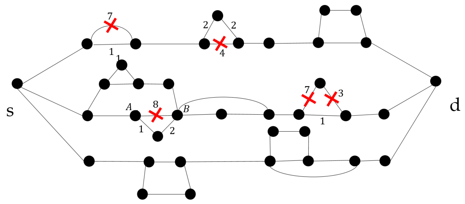
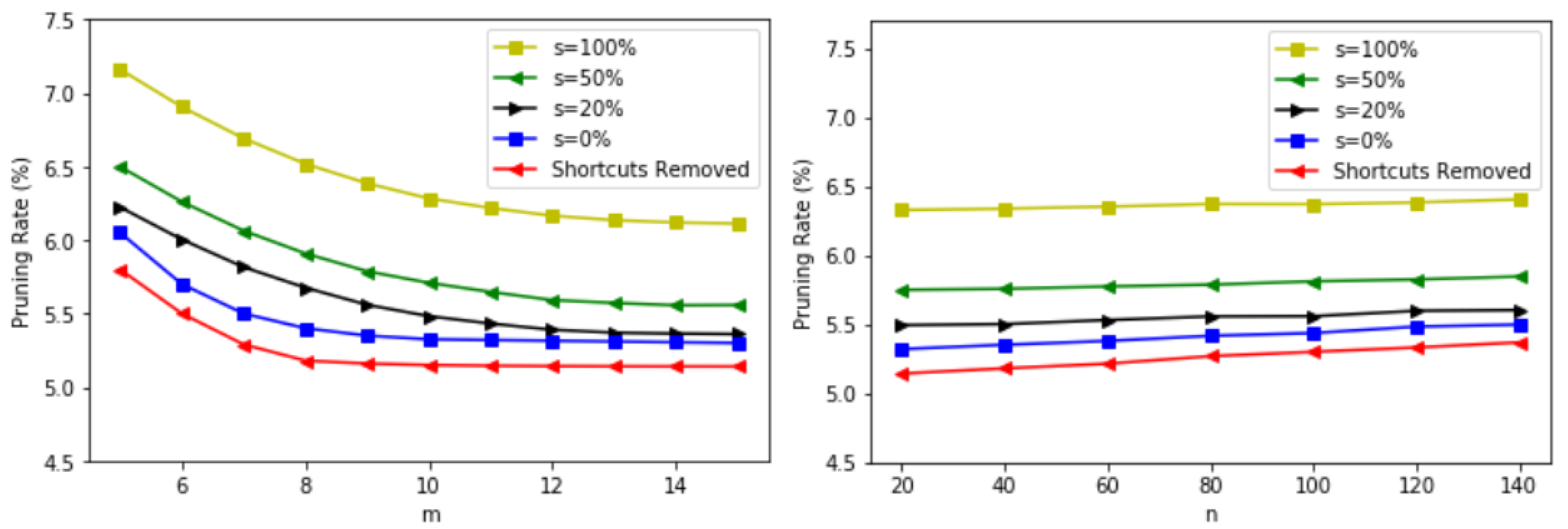
First, we discuss the deterministic case. The simulation covers a wide range of randomly generated SP graphs. The example in Figure 7 shows a case where a number of links is pruned where $m=10$. An instance is the connection between nodes A and B where the link of $g\left(LCM\right\{1,2\left\}\right)$ activation function would completely cover the pruned link of $g\left(8\right)$ activation function. The left plot of Figure 8 shows how the pruning rate deteriorates as the range of the frequencies $[1,m]$ becomes wider. This is due to the fact that as the frequencies range becomes wider, the possibility of getting a link with a $\tau$ value that is divisible by the $\tau$ value of its parallel link (or combination of links) becomes lower. The figure presents a comparison between different percentages of added shortcuts.

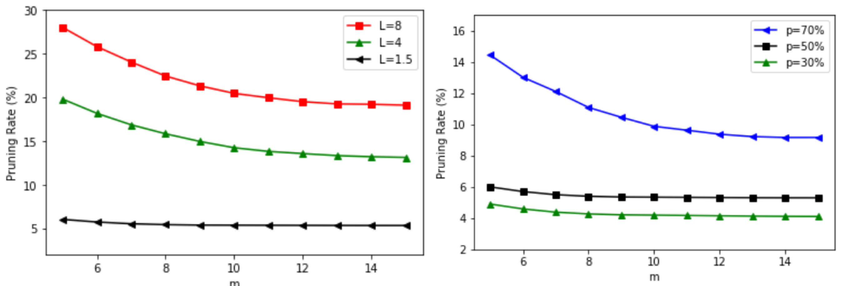
The right plot of Figure 8 shows how the pruning rate slightly increases as the size of the network (represented by the number of link insertions n) becomes larger. This is due to the fact that the average pruning rate of a larger network would not be worse than the average pruning rates of the smaller sub-networks that compromise it. However, combining those small networks to form a larger one would give the chance of having intermediate connecting links that have a chance to be pruned. Eliminating the shortcuts from the network would reduce the pruning rate slightly as those shortcuts typically cover more cases where the links are pruned. For example, having a shortcut with $\tau =1$ makes the whole network parallel to it pruned. Furthermore, the left plot of Figure 9 shows how the expected average degree of parallelism L improves the pruning rate drastically as it would produce a large number of parallel redundant links that would be pruned. The right plot of Figure 9 shows how increasing the number of expected parallel connections in the network with respect to the series connections would increase the pruning rate as most of the pruned links would typically be in a parallel connection.

Now, we discuss the results of the simulation in the probabilistic case.

8.2.1. The High-Clustered Topology

Starting from the simulation results of the high-clustered topology, we see from Figure 10 and Figure 11 the demonstration of the trade-off between the average AoI value and the number of duplicate messages (after a significant time, which is defined as the time until the first copy of the next message is received at the destination node d). This trade-off is shown when we apply the algorithm that prunes the least significant link of the network k times shown on the x-axis.

We find that as the number of links pruned from the network increases, the total average AoI value increases so that the messages are not fresh enough anymore. However, this pruning process leads to avoiding duplicating the messages received at the destination node d within a significant time of the arrival of the first message. The figures in the simulation show that the correlation between the number of pruned links and the average AoI of the network is very strong and near the exponential in the high-cluster topology case. In contrast, the number of duplicate messages decreases in a near-linear proportion.

For the yellow region highlighted in the plots of the simulation, the highlighted area spawns the region of an empirical balance between the number of repeated messages and the total average AoI that the network supports. If the chosen number of the pruned links is within the range of 6–12% of the total number of links in the network.

Even though the shape of the relationship is nearly the same between different values of $\sigma$ and $\mu$, we observe that the higher the value of the standard deviation $\sigma$, the more sensitive the AoI and number of duplicate messages become for the pruning of the network. Furthermore, the sensitivity increases slightly with the increase in the value of $\mu$.

8.2.2. The Low-Clustered Topology

Now, we observe the simulation results of the low-clustered topology. Figure 12 and Figure 13 too demonstrate the trade-off between the average AoI value and the number of duplicate messages received at the destination node d after the time until the first copy of the next message is received at the destination node. Again, the simulation is conducted by running the pruning algorithm multiple times and observing the critical area at which the trade-off settles at balance.

In this case too, the total average AoI value increases in an exponential fashion as the number of links pruned from the network increases. This increase in the number of pruned links makes the network need more time to deliver the messages from node s to node d in a way that renders the received messages less fresh. On the other hand, pruning the messages reduces the number of paths between node s to node d. This reduction in paths leads to reduce the number of duplicate messages received at the destination node d. Figure 12 and Figure 13 show that the correlation between the number of pruned links and the average AoI of the network is near the exponential in the low-cluster topology case, while the number of duplicate messages decreases in a more steep near-linear fashion compared with the reduction in the high-cluster case.

We here too highlight the plots of the simulation to show a region of trade-off that achieves a relatively good reduction in the number of duplicate messages received at d and the total average AoI of the network. This highlighted area spawns the region of this empirical balance between AoI and message redundancy. We see again that the number of pruned links with relative to the total number of links in the network is within the same range shown in the high-clustered topology case.

Furthermore, in this case, we see that the total average AoI becomes more sensitive to the number of pruned links as the value of the standard deviation $\sigma$ increases. On the other hand, we see too that the number of duplicate messages after the significant time becomes more sensitive to the number of pruned links with high values of $\sigma$. Regarding the effect of $\mu$, we see that increasing its value increases the sensitivity of the change of the AoI and the number of duplicate messages too.

8.3. Simulation Summary

After running the simulation that shows the effect of pruning the least significant k links from the network under various different settings, we see in effect the usefulness of our algorithm and its impact on the repetitiveness of the messages delivered at the destination. At the same time, we see the impact of the pruning process on the total AoI of the network and we observe the trade-off between those two characteristics of the network under the different settings.

From the results in Figure 10 and Figure 11, we observe that pruning a small number of links from the network would not impact the total AoI in a drastic way while the impact on the number of duplicate messages is of the same severity that it would be for a higher number of links to be pruned. These results would make it clear that the number of links to be pruned is a parameter to be tuned independently in a way that would sacrifice the AoI for the sake of getting rid of the duplicate messages.

9. Conclusions

Effective non-repetitive routing among nodes in a network is an important function in communication networks. In order to achieve that, pruning the links of the network would be helpful. However, this operation comes with a caveat: it makes the network worse in terms of maintaining the freshness of messages as the defining QoS of the network. In our paper, we studied the case that if a link removal affects the AoI of the messages insignificantly or has no effect, we prune that link. The pruning can be applied to the k least significant links in terms of their impact on the AoI of the messages transmitted in the system. We studied the effect of pruning a number of links on the AoI to reduce the redundancy of the messages that would be received at the destination many times while transmitted only once. We introduced an efficient reduction method designed for series-parallel networks with links of exponentially distributed wait times. In addition, we considered the deterministic case and presented the pruning technique when link removal would not affect the AoI. We showed a pruning algorithm that determines the least significant link in the network, in terms of its effect on the AoI, and prunes it. Lastly, we presented a comprehensive simulation to study the effect of pruning the links on the AoI of the network and the redundancy of messages received by the destination. The main limitation of this work can be concluded in narrowing the study exclusively to SP networks. A potential future direction would be to study the effect of pruning for more general networks.

References

1. Pajevic, S.; Plenz, D. The organization of strong links in complex networks. Nat. Phys. 2012, 8, 429–436. [Google Scholar] [CrossRef] [PubMed]
2. Latora, V.; Marchiori, M. Efficient behavior of small-world networks. Phys. Rev. Lett. 2001, 87, 198701. [Google Scholar] [CrossRef] [PubMed] [Green Version]
3. Albert, R.; Jeong, H.; Barabási, A.L. Error and attack tolerance of complex networks. Nature 2000, 406, 378–382. [Google Scholar] [CrossRef] [PubMed] [Green Version]
4. Bellingeri, M.; Cassi, D.; Vincenzi, S. Efficiency of attack strategies on complex model and real-world networks. Phys. Stat. Mech. Its Appl. 2014, 414, 174–180. [Google Scholar] [CrossRef] [Green Version]
5. Wandelt, S.; Sun, X.; Feng, D.; Zanin, M.; Havlin, S. A comparative analysis of approaches to network-dismantling. Sci. Rep. 2018, 8, 13513. [Google Scholar] [CrossRef]
6. Iyer, S.; Killingback, T.; Sundaram, B.; Wang, Z. Attack robustness and centrality of complex networks. PLoS ONE 2013, 8, e59613. [Google Scholar] [CrossRef] [Green Version]
7. Bellingeri, M.; Bodini, A. Threshold extinction in food webs. Theor. Ecol. 2013, 6, 143–152. [Google Scholar] [CrossRef] [Green Version]
8. Caldu-Primo, J.L.; Alvarez-Buylla, E.R.; Davila-Velderrain, J. Structural robustness of mammalian transcription factor networks reveals plasticity across development. Sci. Rep. 2018, 8, 13922. [Google Scholar] [CrossRef]
9. Bellingeri, M.; Cassi, D.; Vincenzi, S. Increasing the extinction risk of highly connected species causes a sharp robust-to-fragile transition in empirical food webs. Ecol. Model. 2013, 251, 1–8. [Google Scholar] [CrossRef]
10. Zanin, M.; Lillo, F. Modelling the air transport with complex networks: A short review. Eur. Phys. J. Spec. Top. 2013, 215, 5–21. [Google Scholar] [CrossRef] [Green Version]
11. Gallos, L.K.; Cohen, R.; Argyrakis, P.; Bunde, A.; Havlin, S. Stability and topology of scale-free networks under attack and defense strategies. Phys. Rev. Lett. 2005, 94, 188701. [Google Scholar] [CrossRef] [PubMed] [Green Version]
12. Chen, Y.; Paul, G.; Havlin, S.; Liljeros, F.; Stanley, H.E. Finding a better immunization strategy. Phys. Rev. Lett. 2008, 101, 058701. [Google Scholar] [CrossRef] [PubMed] [Green Version]
13. Bellingeri, M.; Bevacqua, D.; Scotognella, F.; Zhe-Ming, L.U.; Cassi, D. Efficacy of local attack strategies on the Beijing road complex weighted network. Phys. Stat. Mech. Its Appl. 2018, 510, 316–328. [Google Scholar] [CrossRef] [Green Version]
14. Tejedor, A.; Longjas, A.; Zaliapin, I.; Ambroj, S.; Foufoula-Georgiou, E. Network robustness assessed within a dual connectivity framework: Joint dynamics of the Active and Idle Networks. Sci. Rep. 2017, 7, 8567. [Google Scholar] [CrossRef] [Green Version]
15. Yates, R.D.; Kaul, S.K. The age of information: Real-time status updating by multiple sources. IEEE Trans. Inf. Theory 2018, 65, 1807–1827. [Google Scholar] [CrossRef] [Green Version]
16. Tang, H.; Wang, J.; Song, L.; Song, J. Minimizing age of information with power constraints: Multi-user opportunistic scheduling in multi-state time-varying channels. IEEE J. Sel. Areas Commun. 2020, 38, 854–868. [Google Scholar] [CrossRef] [Green Version]
17. Yates, R.D.; Sun, Y.; Brown, D.R.; Kaul, S.K.; Modiano, E.; Ulukus, S. Age of information: An introduction and survey. IEEE J. Sel. Areas Commun. 2021, 39, 1183–1210. [Google Scholar] [CrossRef]
18. Costa, M.; Codreanu, M.; Ephremides, A. Age of information with packet management. In Proceedings of the 2014 IEEE International Symposium on Information Theory, Honolulu, HI, USA, 29 June–4 July 2014; IEEE: Piscataway, NJ, USA, 2014; pp. 1583–1587. [Google Scholar]
19. Yates, R.D. The Age of Gossip in Networks. arXiv 2021, arXiv:2102.02893. [Google Scholar]
20. Li, Z.; Shen, H. Utility-based distributed routing in intermittently connected networks. In Proceedings of the 2008 37th International Conference on Parallel Processing, Portland, OR, USA, 8–12 September 2008; IEEE: Piscataway, NJ, USA, 2008; pp. 604–611. [Google Scholar]
21. Xiao, M.; Wu, J.; Liu, C.; Huang, L. Tour: Time-sensitive opportunistic utility-based routing in delay tolerant networks. In Proceedings of the 2013 Proceedings IEEE Infocom, Turin, Italy, 14–19 April 2003; pp. 2085–2091. [Google Scholar]
22. Xue, Y.; Cui, Y.; Nahrstedt, K. A utility-based distributed maximum lifetime routing algorithm for wireless networks. In Proceedings of the Second International Conference on Quality of Service in Heterogeneous Wired/Wireless Networks (QSHINE’05), Lake Buena Vista, FL, USA, 22–24 August 2005; IEEE: Piscataway, NJ, USA, 2005; p. 10. [Google Scholar]
23. Toh, C.K. A novel distributed routing protocol to support ad hoc mobile computing. In Proceedings of the 1996 IEEE Fifteenth Annual International Phoenix Conference on Computers and Communications, Scottsdale, AZ, USA, 27–29 March 1996; IEEE: Piscataway, NJ, USA, 1996; pp. 480–486. [Google Scholar]
24. Ye, Z.; Krishnamurthy, S.V.; Tripathi, S.K. A framework for reliable routing in mobile ad hoc networks. In Proceedings of the IEEE INFOCOM 2003. Twenty-second Annual Joint Conference of the IEEE Computer and Communications Societies (IEEE Cat. No. 03CH37428), San Franciso, CA, USA, 30 March–3 April 2003; IEEE: Piscataway, NJ, USA, 2003; Volume 1, pp. 270–280. [Google Scholar]
25. Zhou, F.; Malher, S.; Toivonen, H. Network simplification with minimal loss of connectivity. In Proceedings of the 2010 IEEE International Conference on Data Mining, Sydney, Australia, 13–17 December 2010; IEEE: Piscataway, NJ, USA, 2010; pp. 659–668. [Google Scholar]
26. Zhou, F.; Mahler, S.; Toivonen, H. Simplification of networks by edge pruning. In Bisociative Knowledge Discovery; Springer: Berlin/Heidelberg, Germany, 2012; pp. 179–198. [Google Scholar]
27. Singh, L. Pruning social networks using structural properties and descriptive attributes. In Proceedings of the Fifth IEEE International Conference on Data Mining (ICDM’05), Houston, TX, USA, 27–30 November 2005; IEEE: Piscataway, NJ, USA, 2005; p. 4. [Google Scholar]
28. Colbourn, C.J.; Xue, G. A linear time algorithm for computing the most reliable source on a series-parallel graph with unreliable edges. Theor. Comput. Sci. 1998, 209, 331–345. [Google Scholar] [CrossRef] [Green Version]
29. Eppstein, D. Parallel recognition of series-parallel graphs. Inf. Comput. 1992, 98, 41–55. [Google Scholar] [CrossRef] [Green Version]
30. Kosta, A.; Pappas, N.; Angelakis, V. Age of information: A new concept, metric, and tool. Found. Trends Netw. 2017, 12, 162–259. [Google Scholar] [CrossRef] [Green Version]
31. Bladt, M. A review on phase-type distributions and their use in risk theory. ASTIN Bull. J. IAA 2005, 35, 145–161. [Google Scholar] [CrossRef]
32. O’Cinneide, C.A. Phase-type distributions and invariant polytopes. Adv. Appl. Probab. 1991, 23, 515–535. [Google Scholar] [CrossRef]
33. Commault, C.; Mocanu, S. Phase-type distributions and representations: Some results and open problems for system theory. Int. J. Control 2003, 76, 566–580. [Google Scholar] [CrossRef]
34. Komárková, Z. Phase-Type Approximation Techniques. Ph.D. Thesis, Masarykova Univerzita, Fakulta Informatiky, Brno, Czechia, 2012. [Google Scholar]
35. Papoulis, A.; Saunders, H. Probability, Random Variables and Stochastic Processes; Tata McGraw-Hill Education: New York, NY, USA, 1989. [Google Scholar]
36. Raju, C.K. Products and compositions with the Dirac delta function. J. Phys. Math. Gen. 1982, 15, 381. [Google Scholar] [CrossRef]
Figure 1. (a) The operation composition in parallel denoted by C p . (b) The operation composition in series denoted by C s . (c) a sample SP graph that is represented as three parallel paths: P 1 P 2 P 3 , where P 1 : [ 1 , 2 3 , [ [ 4 , 5 6 ] [ 7 , 8 ] ] , 9 ] . P 2 : [ 10 11 , 12 ] . P 3 : [ 13 ] .
Algorithms 15 00228 g001
Figure 2. The progression of AoI in our model.
Algorithms 15 00228 g002
Figure 3. Links deliver probabilistically under the exponential distribution with expected delivery times of 1 / λ 1 , , 1 / λ n after the arrival of the message to the source node. (a) is parallel links reduction. (b) is series links reduction.
Algorithms 15 00228 g003
Figure 4. The complete coverage in the deterministic case, link 4 is completely covered by both links 1 and 2 together. Hence, it can be completely pruned. (a) shows a simple source-destination network resembling an example. (b) shows the times at which each link transmits where the fourth one is completely covered by the rest.
Algorithms 15 00228 g004
Figure 5. Flowchart showing the process of determining the weakest link in the probabilistic case.
Algorithms 15 00228 g005
Figure 6. The topologies used in the probabilistic example. (a) is the low-clustered topology. (b) is the high-clustered topology.
Algorithms 15 00228 g006
Figure 7. An example of pruning in the deterministic case.
Algorithms 15 00228 g007
Figure 8. The pruning rate in the deterministic case where L = 1.5 , p = 50 % . For the left plot n = 20 , for the right plot m = 10 .
Algorithms 15 00228 g008
Figure 9. The pruning rate in the deterministic case where n = 20 , s = 0 % . For the left plot p = 50 % , for the right plot L = 1.5 .
Algorithms 15 00228 g009
Figure 10. The simulation results from running the pruning algorithm on the high-clustered topology when μ = 1 . The left column is the result after running the algorithm when σ = 1 and the right column is the result after running the algorithm when σ = 2 .
Algorithms 15 00228 g010
Figure 11. The simulation results from running the pruning algorithm on the high-clustered topology when μ = 2 . The left column is the result after running the algorithm when σ = 1 and the right column is the result after running the algorithm when σ = 2 .
Algorithms 15 00228 g011
Figure 12. The simulation results from running the pruning algorithm on the low-clustered topology when μ = 1 . The left column is the result after running the algorithm when σ = 1 and the right column is the result after running the algorithm when σ = 2 .
Algorithms 15 00228 g012
Figure 13. The simulation results from running the pruning algorithm on the low-clustered topology when μ = 2 . The left column is the result after running the algorithm when σ = 1 and the right column is the result after running the algorithm when σ = 2 .
Algorithms 15 00228 g013
Publisher’s Note: MDPI stays neutral with regard to jurisdictional claims in published maps and institutional affiliations.