Exploring the Efficiencies of Spectral Isolation for Intelligent Wear Monitoring of Micro Drill Bit Automatic Regrinding In-Line Systems

Abstract

Despite the increasing digitalization of equipment diagnostic/condition monitoring systems, it remains a challenge to accurately harness discriminant information from multiple sensors with unique spectral (and transient) behaviors. High-precision systems such as the automatic regrinding in-line equipment provide intelligent regrinding of micro drill bits; however, immediate monitoring of the grinder during the grinding process has become necessary because ignoring it directly affects the drill bit’s life and the equipment’s overall utility. Vibration signals from the frame and the high-speed grinding wheels reflect the different health stages of the grinding wheel and can be exploited for intelligent condition monitoring. The spectral isolation technique as a preprocessing tool ensures that only the critical spectral segments of the inputs are retained for improved diagnostic accuracy at reduced computational costs. This study explores artificial intelligence-based models for learning the discriminant spectral information stored in the vibration signals and considers the accuracy and cost implications of spectral isolation of the critical spectral segments of the signals for accurate equipment monitoring. Results from one-dimensional convolutional neural networks (1D-CNN) and multi-layer perceptron (MLP) neural networks, respectively, reveal that spectral isolation offers a higher condition monitoring accuracy at reduced computational costs. Experimental results using different 1D-CNN and MLP architectures reveal 4.6% and 7.5% improved diagnostic accuracy by the 1D-CNNs and MLPs, respectively, at about 1.3% and 5.71% reduced computational costs, respectively.

1. Introduction

Maintenance costs have been shown in recent studies [1,2,3] to contribute a significant portion of total operating costs. This has motivated industries towards integrating cost-efficient technologies (and practices) into their daily operations. In addition to this perspective, safety and reliability are often prioritized for ensuring maximum profit, maintaining ethical obligations, minimizing downtime, and achieving optimal utility of equipment [2,3,4]. As a consequence, intelligent equipment and tool monitoring, fault diagnosis, and prognostics are currently being integrated into maintenance management modules, and thanks to artificial intelligence (AI), intelligent monitoring has gradually attracted attention from industries since they require little or no domain knowledge, are user-friendly, and offer minimal false alarm rates [4,5].

In the modern manufacturing industry, high-density packaging technologies have become an unavoidable requirement. The design of printed circuit boards (PCB) demands high-precision cutting and drilling of small holes (as small as 0.1 mm or less), which requires the use of micro drill bits [6]. Due to prolonged usage, the micro scale, hole-location errors, reaming, and their brittle and delicate nature, drill fractures/breakage often occur during the drilling process. More often than not, these drill bit failures can be traced to the high-frequency vibrations generated during the drilling process; therefore, the demand regular tool monitoring and maintenance—regularly sharpening [7]. Most investigations on the vibration of micro drilling are focused on only drill self-structure. However, it is also important to monitor the maintenance efficiency of the drill bit regrinding machine to ensure that at all times, the drill bits produce the desired surface finish and geometrical accuracy of the finished workpiece—PCB.

Several direct, indirect, and/or hybrid tool monitoring techniques/technologies have been studied [8,9]. Direct methods such as optical devices and cameras, although more reliable for accurate monitoring, are faced with certain limitations. Their real-time usability may be affected since ARIS wheels rotate at high speeds and may produce unclear images in real-time, which often require interrupting the machine. Further, finding an optimal camera localization point is another major challenge. Against these limitations, indirect methods—cutting force, acoustic emission, spindle motor, temperature, vibration, machining sound, etc.—offer real-time efficiencies and the integration of multiple sensing opportunities for fully extracting deep and shallow machine behavior for optimal condition monitoring [7]. In addition, recent technological advancements have ushered in intelligent algorithms and the super computational resources for harnessing them—for intelligent tool monitoring [4]. These intelligent algorithms, such as convolutional neural networks (CNN) [5], recurrent neural networks (RNN), auto encoders (AE) [10], and MLPs [11], are quite robust for diverse predictive maintenance and equipment monitoring purposes and have been reported in many studies, including but not limited to hydraulic equipment monitoring [5], remaining useful life estimation, wear detection [7], and machinery fault diagnostics and prognostics [12,13]. Unlike the traditional Bayesian methods that require a significant level of hand-crafted discriminative and/or non-discriminative feature extraction as the case study demands, these intelligent algorithms—deep learning (DL) models—are designed to accept raw sensor inputs and follow a series of advanced mathematical processes for automatic feature extraction and predictive modeling in a comprehensive framework with less dependence on domain knowledge. Nonetheless, finding a balance between computational costs and accuracy remains a challenge, especially for real-time cases where both factors play major roles in the decision-making, selection, and deployment.

Although highly efficient, the accuracy of these intelligent algorithms for discriminative tasks are sometimes threatened by a high similarity in the sensor signals across different tool health conditions [5,14]. Unfortunately, this is often the case of micro drill bit regrinding machines because the grinding wheel wear conditions are usually mixed with the high-frequency components with low amplitudes, and that makes it hard to identify/isolate. This opens up the need for spectral isolation—extraction of signals within a finite frequency band from a mixed signal. Interestingly, different signal processing tools abound for frequency-domain and/or time-frequency-domain analyses; however, the fast Fourier transform (FFT) retains its traditional advantages—computational cost advantage, user-friendly visualization for inferences, minimal modeling assumptions for spectral isolation, and support for power spectral density (PSD) computation for improved signal analyses/processing [7,15,16]. This has motivated us to explore its efficiencies alongside intelligent classifiers for vibration-based wear monitoring of high-frequency automatic regrinding in-line equipment. The following highlights are the major contributions of this study:

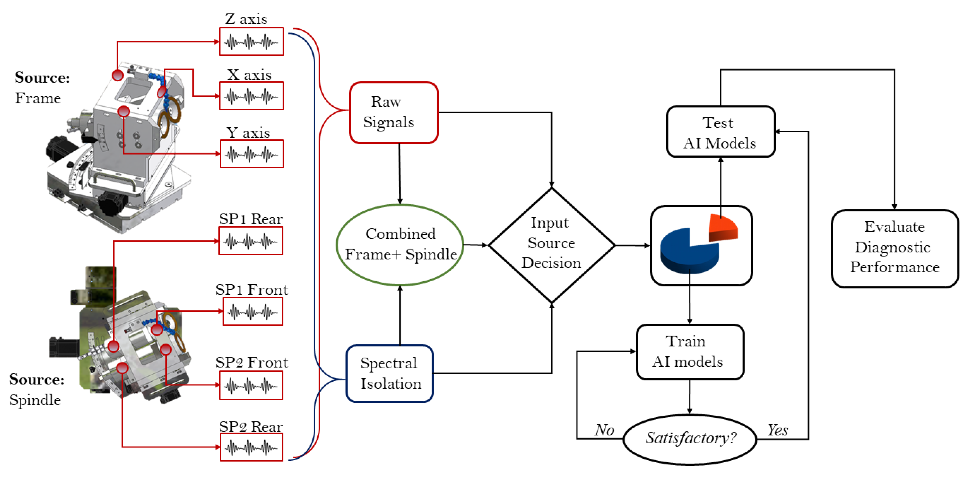
• A multi-sensor vibration monitoring system is proposed for the automatic micro drill bit regrinding of in-line equipment. The proposed framework adopts spectral isolation by integrating the low-frequency vibration responses from the regrinding frame and the high-frequency vibration responses from the gas bearing-powered regrinding spindle in a comprehensive manner. These provide highly discriminate information from the regrinding frame and the regrinding spindle, respectively, for improved condition monitoring.
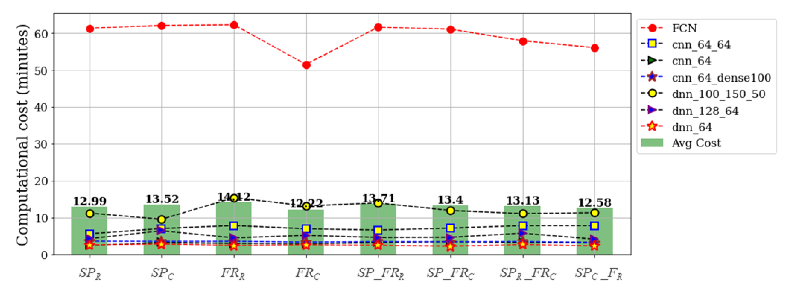
• A multi-option diagnostic framework that exploits the multiple sensor data’s vulnerabilities is proposed. The framework offers the options of choosing different data sources—stand-alone and/or integrated sensor data and exploits different 1D-CNN and MLP model architectures. This presents an avenue for evaluating the efficiencies of spectral isolation for improved tool wear monitoring and for assessing the computational cost implications of employing the proposed intelligent monitoring technology.
• For the proposed study, we leverage experimental data from an ultra-precision micro drill bit automatic regrinding in-line system (ARIS), which regrinds micro drill bits ($\varphi 0.15$–$\varphi 0.075$ mm) used in the PCB manufacturing process. Empirical and descriptive conclusions are drawn following extensive investigations and evaluations. Our research offers a reliable framework for future research and practice in real-time industrial monitoring/diagnostic applications.

The remainder of this paper is structured as follows: Section 2 discusses motivation for the proposed study and related Works, while Section 3 provides the the background of study. Section 4 presents the experimental assessment, while Section 5 concludes the paper.

2. Motivation for Proposed Study and Related Works

Precision drilling, which requires an accurate drilling process, ensures a high-quality product; however, it is essential to understand the condition and dynamic performance of a drill bit in a drilling process, especially for high-speed micro drilling, to reduce the risk of hole-location errors, reaming fractures, and drill fractures [6]. Although only a few studies have examined the dynamics of drilling processes that result in undesirable effects, such as chatter and drill breaks, most studies have shown that breakage is the most common cause of drill failure, and this is most often traced to excessive drilling forces in the drilling process, as well as drill bit bluntness [17,18]. Cutting chip geometry and symmetry can significantly affect the cutting and dynamic properties of a drill bit. Even the tiniest variation in the complex geometry or symmetry of a cutting chip can significantly affect the cutting and dynamic properties of a drill bit.

As the recent industry 4.0 revolution becomes more apparent, which interestingly features micro (nano) technological advancement (amongst many other technologies), PCB production requirements are prioritizing higher cost efficiency, which invariably implies that PCBs are becoming smaller in size. This also implies a reduction in hole sizes on these PCBs to accommodate for the numerous micro chips and electronic units [19]. Unlike the past PCB holes that featured a minimum diameter of $\varphi 0.2$ mm, recent PCBs feature more miniature holes that are ($\varphi 0.15$–$\varphi 0.075$ mm) in diameter and are in higher demand. Unfortunately, these micro drill bits are difficult to regrind and are often scrapped after use. Therefore, it becomes imperative to devise reliable regrinding solutions that would minimize drill breakage, hole-location errors, reaming fractures, and drill fractures. Interestingly, the micro drill bit ARIS developed by Instern Co. Ltd., Seoul, Korea, offers a highly reliable (intelligent) solution for regrinding micro drill bits with high efficiency and durability [19]; however, amidst its efficiencies, due to the micro scale of these drill bits, the regrinding wheel surface of these high-precision regrinding systems should be monitored for wear. This is because there is a high positive correlation between the grinding wheel surface wear and poor cutting chip geometry and symmetry.

On the one hand, vibration monitoring has, by far, been proven across diverse applications to be effective for condition monitoring applications [5,12]. This is because most industrial equipment produces different ranges of mechanical vibrations during operation, which change as the equipment operating/health condition changes. On the other hand, the abundance of signal processing techniques provide conventional paradigms for understanding the spectral changes in the vibration signals using advanced computational methods, such as FFT, mel frequency cepstral coefficients, and wavelet transform [20]. Interestingly, the regrinding system’s vulnerabilities to mechanical vibration offer an avenue for critically isolating unique (discriminative) frequency bands in the signals for accurate condition monitoring to ensure drill bit safety and retain acceptable drill bit efficiencies while achieving desired cost benefits. For instance, Lee et al. [7] explored the efficiencies of the FFT algorithm for isolating (denoising) auditory signals from the grinding wheel of a G50150 Automatic Surface Grinder machine to enhance the accuracies of a deep learning-based diagnostic model for wear monitoring. By isolating the discriminative frequency bands between 300 and 500 Hz, they were able to provide intelligent diagnostic support to assist operators in determining whether the grinding wheel was worn or not. Moreover, the authors of [15] proposed a comprehensive high-frequency vibration monitoring system for incipient fault detection and the isolation of gears, bearings and shafts/couplings in turbine engines and accessories, which feature a time synchronous averaging (TSA)-based denoising technique for noise reduction from events unrelated to the component of interest. These and many other studies reflect not just the efficiencies of spectral isolation as a denoising technique, but they also provide a verifiable rationale for developing computationally cost-effective and intelligent modeling, on the one hand, and improved discriminative modeling, on the other hand. In this domain, it may become an uphill task to determine which denoising technique is the most effective (considering all evaluation perspectives). However, the FFT offers a reliable solution for identifying critical frequency components in a signal [15,16].

In contrast to traditional Bayesian methods, DL models offer superior intelligent modeling efficiencies and are skewing reliability studies (and applications) on industrial cyber-physical systems (ICPSs) as a consequence of the increasing complexity of processes and systems and the inherent necessity to model them [5]. Process efficiencies, equipment condition monitoring, spatiotemporal forecasting, and many other solutions have been recently improved as a result of this shift to DL-based support [21,22,23,24,25]; however, some issues remain, including over-fitting and interpretability issues, optimal hyperparameter selection/optimization, standardized weight initialization paradigm, and discovering the optimal decision criteria between power consumption and performance [4,26]. In spite of this, given the necessity of providing accurate real-time solutions for ICPS components, and especially considering the growing need for uncertainty modeling, sensor data discrepancies, and dynamic operating conditions, DL techniques remain preferable even at the expense of computational power. In this light, numerous DL-based algorithms have been developed over the years, including, but not limited to the RNNs and echo state networks for time-series forecasting [21,22,23], CNNs for discriminative modeling/diagnostics [5,24], and the multi-purpose DNNs [5,11]. Most of these algorithms are stand-alone models that obviously come with their shortcomings and may be component-specific and/or application-specific. Moreso, the task presented herein clearly points at the CNNs and MLPs as possible solutions considering that their architecture are fundamentally designed for discriminative modeling and/or classification purposes (even though MLPs can also model regression/forecasting problems accurately). In this quest, our study explores different architectures of these algorithms for the proposed case study. This is particularly necessary considering that different model architectures (number of layers and hyperparameters) invariably produce different results at different computational costs [5,11]. Actually, the deeper the model architecture, the higher the probability of over-fitting and computational cost (and vice versa). By exploring different architectures of the models, we may provide an empirically strong rationale for validating the impact of spectral isolation for improved condition monitoring/diagnostics on the one hand and the choice of, and recommendation for, the appropriate DL model(s) on the other hand, while considering ease-of-use, real-time applicability, and other necessary factors.

3. Background of Study

In detail, this section discusses the core components that constitute our study—the working principle of the micro drill bit ARIS, the proposed monitoring framework, and an overview of its sub-components.

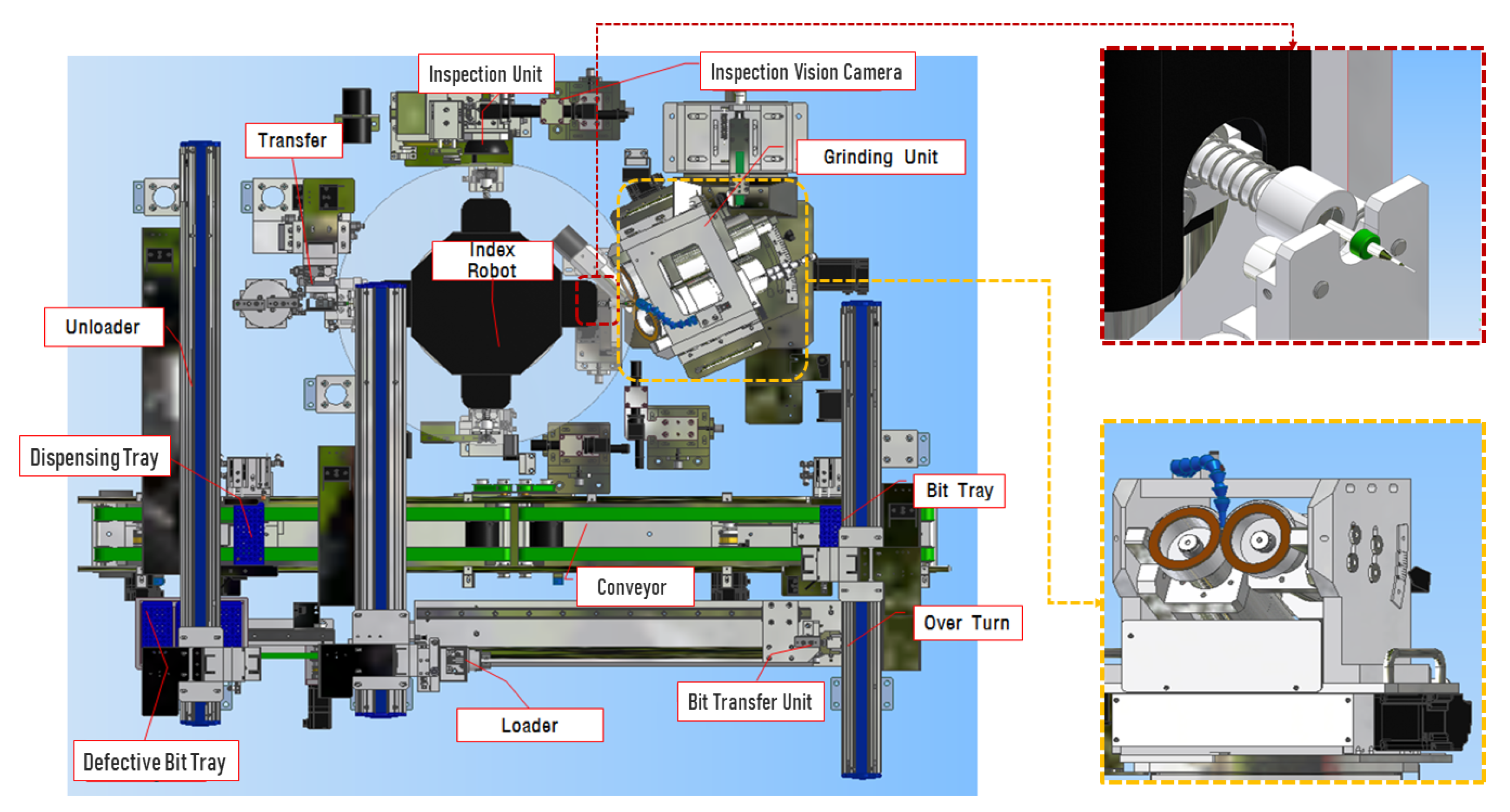
3.1. Working Principle of the G50150 Micro Drill Bit ARIS

The working process of the micro drill bit ARIS is fundamentally robotic—it repeats the tasks for a single micro drill bit at a time: loading, grinding, optical inspection/scanning, and unloading [19]. Figure 1 shows the functional plan view of the G50150 micro drill bit ARIS and the key components of interest—the collet and regrinding unit.

As shown in Figure 1, the G50150 micro drill bit ARIS has many components—each serving high-precision functions for an accurate (and well-timed) regrinding process. From the bit transfer unit, the drill bits (stacked in crates) are loaded onto the conveyor, where the index robot intelligently picks the drill bits (one at a time) with the help of the collet (highlighted in a red dotted square). Once a drill bit is picked, the index robot rotates 90 degrees in an anti-clockwise direction such that the drill bit faces the grinding unit (highlighted in a yellow dotted square). The grinding unit houses the two regrinding wheels spinning in opposite directions and are powered by high-speed gas bearings. With the help of its mobile base, it moves closer to the collet such that the spinning grinding wheels make contact with the drill bit’s heel alternatively. By so doing, some of the drill bit’s heel wears off, thereby sharpening its cutting edges, lips, and chisel.

Next, the index robot rotates again by 90 degrees in an anti-clockwise direction such that the sharpened drill bit faces the inspection unit—a high-resolution camera-based inspection system that captures the drill bit’s cutting surface for the operator’s visual inspection via a PC’s display unit. After yet another 90-degree rotation in the anti-clockwise direction, the reground (and visually inspected) drill bit is collected by the transfer unit to the unloader, which is carefully collected on the dispensing tray in crates. The cycle continues for all the drill bits in the crate. As the grinding operation continues and the drill bit comes in contact with the grinding wheels, the regrinding surface gradually wears to a point—end-of-life (EoL)—where it is no longer recommended for use. Meanwhile, high-frequency responses are generated and can be captured via high-sensitivity accelerometers. If the grinding process is repeatedly performed for a long time and the grinding wheels approach EoL, their respective cutting power is greatly reduced, and this results in poor grinding operations, which may even cause the drill bits to break.

3.2. Proposed Intelligent Monitoring Framework

As an alternative to the use of raw vibration signals from the grinding unit, the proposed framework offers a computationally cost-efficient approach—spectral isolation by integrating the low-frequency vibration responses from the regrinding frame and the high-frequency vibration responses from the gas bearing regrinding spindle in a comprehensive manner. These provide highly discriminate information from the regrinding frame and the regrinding spindle, respectively, for improved diagnostics/wear detection efficiencies in addition to improved computational costs. Figure 2 illustrates the proposed intelligent monitoring framework.

As shown, the framework accepts vibration signals from seven accelerometers—three (3) affixed to the regrinding unit’s frame in the X-, Y-, and Z-axes, while the remaining four (4) are affixed under the two regrinding spindles in their front and rear positions, respectively. This provides a comprehensive source of vibration measurements for monitoring. A key module of the proposed model is the input source decision module, which provides the user with the option of choosing the source sensors for use. One may choose only the raw spindle signals, only the raw frame signals, a combination of both raw signals, or employ the spectral isolation technique as a preprocessing step before inputting the signals. The following subsections provide insights into the framework’s key modules—spectral isolation and DL-based diagnostic models.

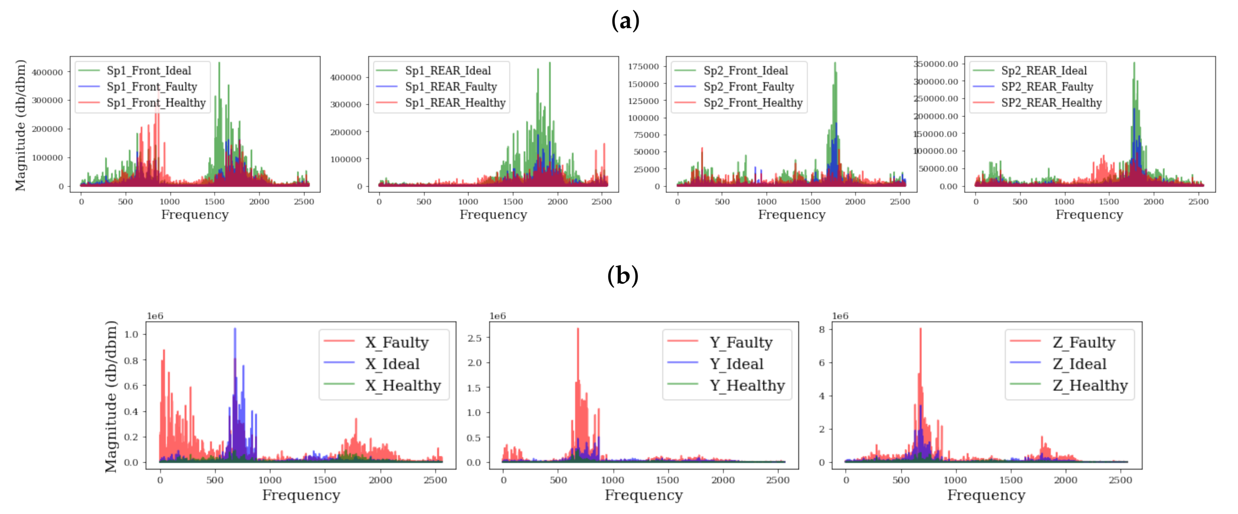
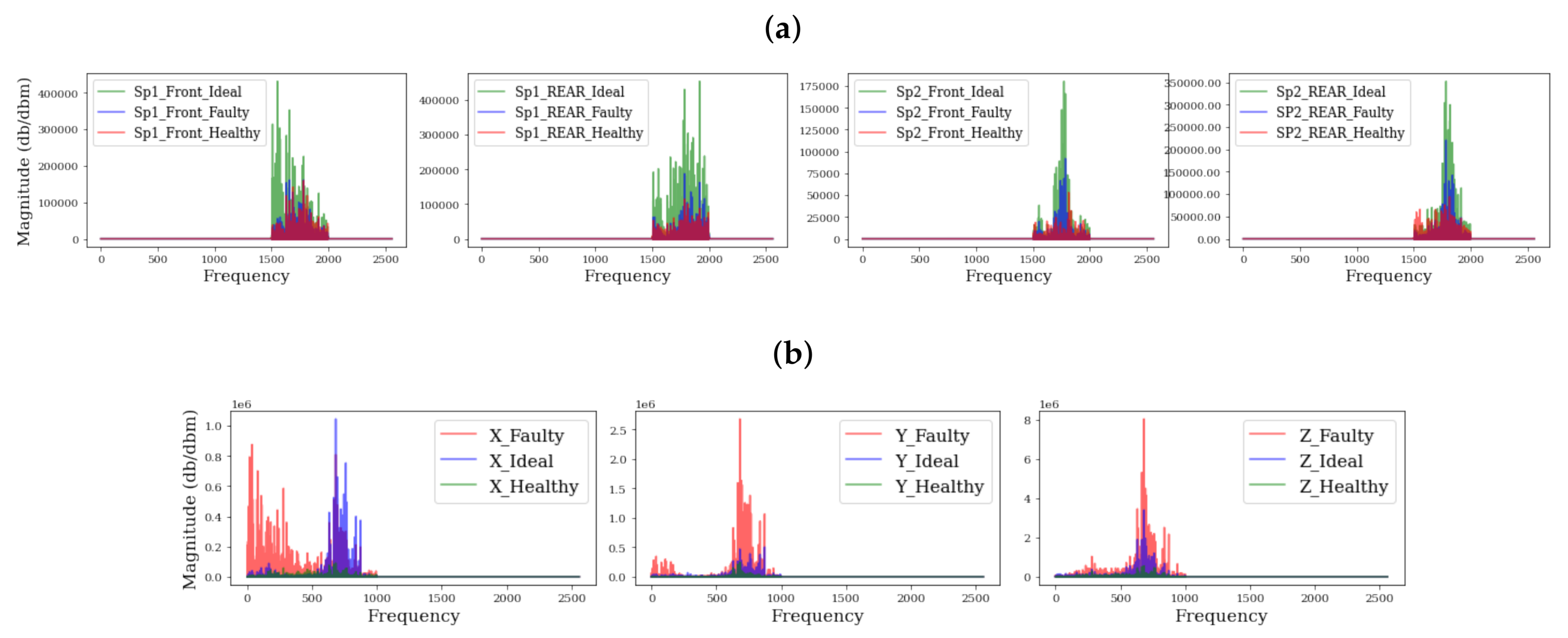
3.2.1. FFT-Based Spectral Isolation

In addition to providing more reliable paradigms for both stationary and non-stationary signals, the invention of various frequency-domain (and time-frequency-domain) techniques provides a solution to the limitations of time-domain methods of digital signal processing (DSP). Named after Joseph Fourier (21 March 1768–16 May 1830), the Fourier transform (and its variants) forms the basis for most frequency-domain signal processing techniques [7,15]. As DSP tools, the FFT and PSD provide a reliable avenue for analyzing the spectral behavior of signals. While FFTs can flourish reliably under relaxed assumptions because most signals are comprised of a complex synthesis of Sine and Cosine functions, the PSD offers an even more reliable alternative to the FFT due to its comparatively higher sensitivity to spectral changes in a signal. This is because the FFT has high sensitivity and outputs a wide range of frequencies (including insignificant ones) that constitute a signal, and due to this high sensitivity, it is sometimes inefficient in monitoring conditions accurately. In addition, the PSD computes the energy densities of the constituent frequencies, thereby exaggerating the relevance of high-energy signal components while suppressing the effects of the lower-energy constituents.

Given a time-record (one-dimensional sensor signal) $f\left(x\right)=\left\{x_1,x_2,\dots ,x_m\right\}$, the Fourier transform of a function $f\left(x\right)$ is traditionally denoted $F\left(k\right)$ and is computed using Equation (1) below:

$$F\left(\omega \right)={\int }_{-\infty }^{\infty }f\left(x\right)e^{-i\omega x}dx$$

(1)

where $f\left(x\right)$ is the input signal, w is the length of the transform, and $F\left(w\right)$s is the corresponding frequency-domain output of the signal.

The idea behind spectral isolation is to emphasize the critical frequency bands while moderately reducing the interference of noise and other irrelevant frequency sources. This requires knowledge of the target system’s spectral behaviors and identifying the critical frequency bands peculiar to the equipment’s operating conditions. Isolating these critical frequencies entails that the interfering frequency bands are muted (reduced to zero magnitudes).

Suppose one wants to retain the critical frequency segment ranging from ${\omega }_a$ to ${\omega }_b$ (where $0\le {\omega }_a\le {\omega }_b\le \left|\omega \right|$) by creating a filter that eliminates a range of frequency bands—${\omega }_c\in \left|\omega \right|\notin \{{\omega }_a\to {\omega }_b\}$, we will specify a box-shaped frequency response with cutoff frequency $\{{\omega }_a\to {\omega }_b\}$ such that:

$$F_{a\to b}\left(\omega \right)=\left\{\begin{array}{cc}1\hfill & \{{\omega }_a\to {\omega }_b\}\hfill \\ 0\hfill & {\omega }_c\hfill \end{array}\right.$$

(2)

Subsequently, the inverse FFT (iFFT) will be applied to transform the frequency segment (critical frequencies) back to a time domain. The iFFT of $F_{a\to b}\left(\omega \right)$ is then computed using Equation (3) below:

$$f\left(x_{a\to b}\right)=\frac{1}{2\pi }{\int }_{-\infty }^{\infty }{F}_{a\to b}\left(\omega \right)e^{i\omega x}d\omega$$

(3)

where $\omega$ ranges between ${\omega }_a$ to ${\omega }_b$.

Finally, the iFFT-transformed signals in the time domain, which only preserves the critical frequency segment, will be used as the most discriminating signals (inputs) for diagnostic modeling.

3.2.2. Standard DL-Based Diagnostic/Classification Models

Traditional classification algorithms (e.g., support vector machine, decision trees) require preprocessing in order to extract discriminative features. This often creates too much room for expensive statistical assumptions peculiar to the feature extraction method; amidst the limitations of the traditional classification algorithms. On the bright side, DL-based algorithms offer better classification accuracies, ease-of-use, and automatic feature extraction capabilities.

Amongst the many standard DL algorithms, CNNs and MLPs are the most popular for accurate discriminative modeling efficiencies. While CNNs are unique for their working principle—mimicking the human visual cortex for discriminative feature extraction and identification of labels (objects, conditions, etc.), MLPs comprise nodes/neurons that perform tasks via a feedforward activation learning process [5]. CNNs are quite popular for many diagnostic/detection problems, including, but not limited to wear detection and pattern recognition [27]. This efficiency emanates from the convolving (Conv) and pooling layers, which function as filters for high-level (automatic) feature extraction; and with the fully connected layer(s), its architecture can be modified for better diagnostic accuracies. On the other hand, MLPs comprise two or more multi-layer perceptrons—a class of feedforward artificial neural network that consists of at least three layers of nodes: an input layer, a hidden layer, and an output layer, whereby the supervised training process is achieved via a backpropagation learning process with the aid of nonlinear activation functions [5].

Given a set of one-dimensional vibration measurements as inputs— $X_n^{{}^{\prime }m}=\{(x_1^{\prime },y_1),(x_2^{\prime },y_2),...,(x_n^{\prime },y_n)\}$, where $x_n^{\prime }\in R^m$ and $y_n\in \{0,1,...,n\}$, the convolution layer performs a convolution operation on the data through a convolution kernel, and then adds a bias and activation function to finally form a corresponding convolution feature map:

$$h_{2,j}=f(\sum _{i=1}^r{X}_{ni}^{{}^{\prime }m}\ast W_j+b_j)$$

(4)

where $X_{ni}^{{}^{\prime }m}$ represents the i-th channel of the input data (a total of r channels), $W_j$ is a weight matrix, $b_j$ is the bias, * indicates convolution operation, and f is an activation function that ranges across popular functions, such as the Sigmoid, Tanh, and rectified linear unit (ReLU) [28].

On the other hand, consider an MLP with l hidden layers with a varying real integer number of nodes in each layer such that the nodes $a_1^{l-1},a_2^{l-1},\dots ,a_r^{l-1}$} are in the $l-1th$ hidden layer. They first receive activated outputs from the nodes in the preceding layer—$l-2th$ layer via a forward propagation process and compute yet another activated output to the nodes in the final hidden layer—the $l_{th}$ hidden layer. The forward propagation continues from the input layer nodes to the nodes in the output layer $O_{i_{\mathrm{out}}}$, which is then followed by a backpropagation process (by updating the weights and biases) to minimize the cost function by either a stochastic gradient descent algorithm, Adam [29] optimizer, and/or any of the quasi-Newton algorithms [30].

Empirically, the inputs $O_{i_{\mathrm{in}}}$ provided by the node $a_i^l$ are received by the nodes $O_i$ are given by the sum of the activated outputs of $a_i^l$ multiplied by the corresponding connection weight matrix $w_l$ using Equation (5).

$$O_{i_{\mathrm{in}}}=\sum _{i=1}^r{w}_l\ast A\left[\mathbf{i}\right]$$

(5)

where A[i] is the activated outputs of the nodes in the $l_{th}$.

The output $O_{i_{\mathrm{out}}}$ from each of the output nodes $O_i$ is obtained by passing the inner product $O_{i_{\mathrm{in}}}$ through a nonlinear activation function f using Equation (6):

$$O_{i_{\mathrm{out}}}=f\left(O_{i_{\mathrm{in}}}\right)$$

(6)

The automatic (supervised) learning process of the CNN and MLP enables the minimizing of the squared error in the predicted outputs and the actual target labels using Equation (7):

$$E={\left(y-O_{i_{\mathrm{out}}}\right)}^2$$

(7)

where E is the prediction error (cost function), and y is the desired output label.

More often, the ReLU activation function is preferred because of its faster learning advantages on DNNs. Further, because it returns the corresponding output value for positive values whereas, for negative input values, it returns a zero value [28]; and ideally, most input variables—extracted features are usually greater than zero—the ReLU is often preferred.

4. Experimental Assessment

For the proposed investigation, we leverage experimental data from a micro drill bit ARIS (model TGM-1011) manufactured by Instern Co. Ltd., Korea. The equipment automatically regrinds micro drill bits ($\varphi 0.15$–$\varphi 0.075$ mm) used for PCB manufacturing process via a series of ultra-precision control mechanisms.

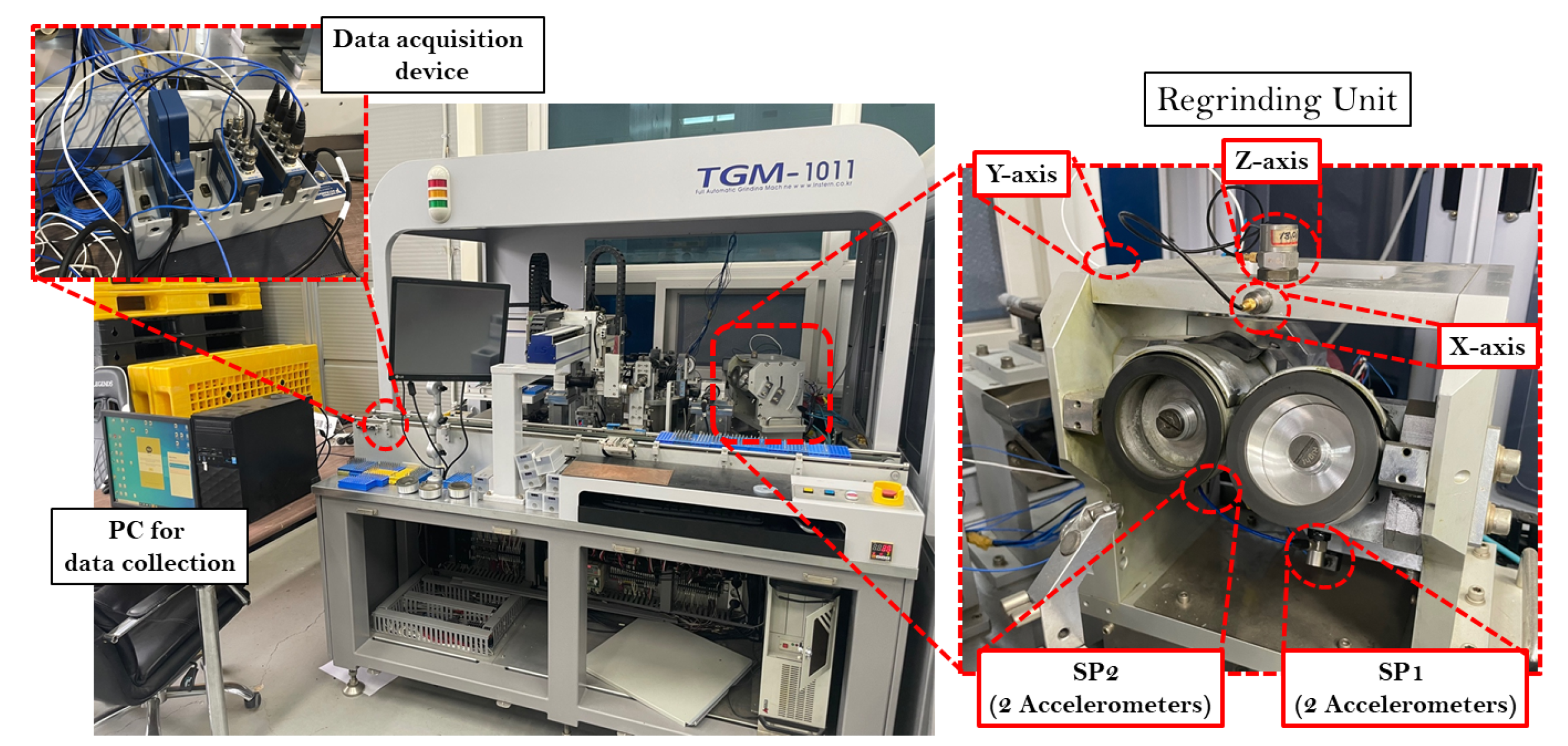
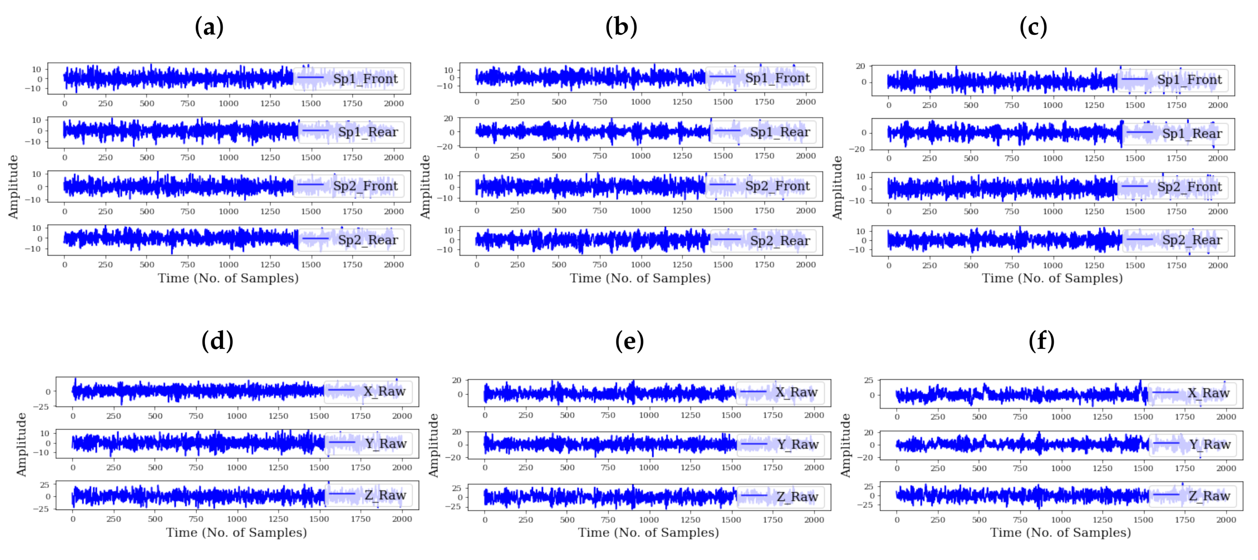
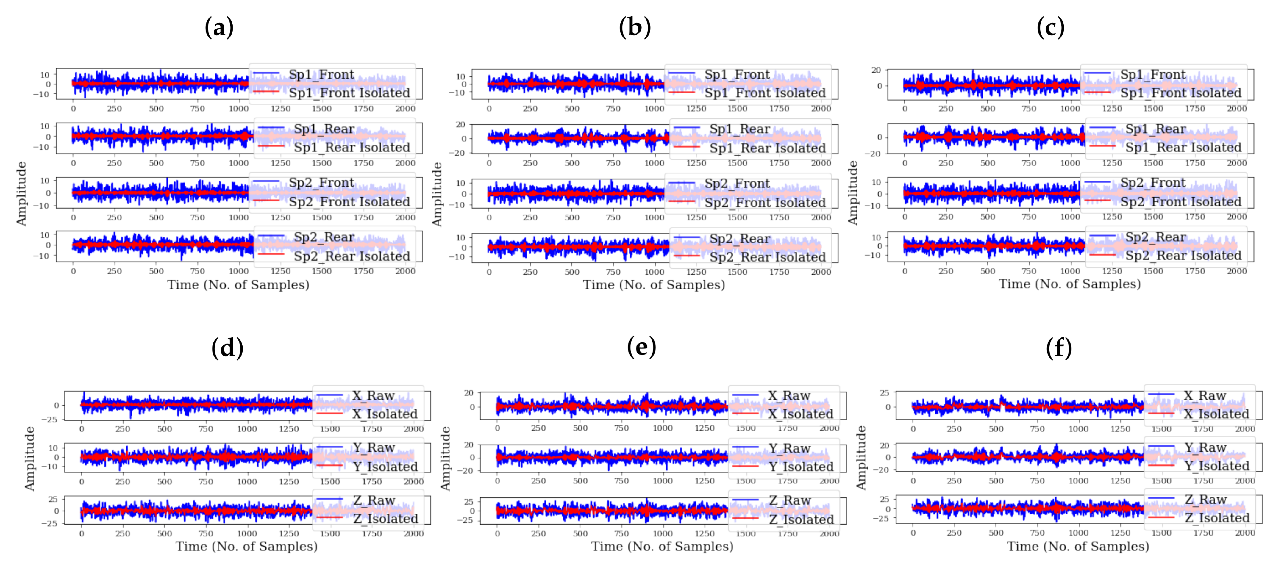
4.1. Data Acquisition and Spectral Isolation

For the proposed study, seven (7) high-sensitivity accelerometers were mounted on the grinding unit at different locations—four (4) under the two high-speed spindles and three (3) on the X-, Y-, and Z-axes of the top frame. Figure 3 shows the actual equipment and the sensor positions.

The accelerometers were connected to two NI 9228 modules affixed to a NI cDAQ 9178, and with the help of a LabView software, the digital vibration signals were collected at a sampling rate of 1 KHz. Three different pairs of grinding wheels corresponding to the three major health stages of the wheels are labeled—healthy (new pair of grinding wheels), fairly used (about 40–50% life remaining useful life left for the wheel pair), and faulty (about 0 - 10% remaining useful life left for the wheel pair). Figure 4 shows a picture of the wheels at the different health stages.

It can be observed from Figure 4a–c that the grinding surface of the wheels wears down due to prolonged usage. This obviously affects their grinding performance and may damage the micro drill bits as the wheel surface wear intensifies. For each of the wheel conditions, vibration signals were collected and stored in their respective folders and employed on the proposed intelligent wear monitoring framework. Figure 5 presents a view of the raw vibration signals, while Figure 6 shows the spectra comparison of the signals from the different wheel health stages.

It is observed from Figure 5a–d that the regrinding spindles/wheels’ responses are concentrated in the higher frequency bands (between 0 and 1000 Hz) while the frame’s responses are concentrated in the lower frequency bands (between 1500 and 2000 Hz). This presents the opportunity for isolating the critical segments to minimize computational costs, improve diagnostic accuracy, and minimize classifier confusion. Our study proposes the FFT-based spectral isolation technique, and was deployed on the signals. Figure 7 shows the critical segments of the respective components (spindle and frame), while Figure 8 shows their corresponding time-domain signal outputs after the spectral isolation process.

As shown in Figure 7, it can be observed that the discriminance in the magnitudes for the different grinder health states is obvious. Moreover, it can be observed in Figure 8 that the signals’ amplitudes are reduced while preserving the important periodic components of the signals. By harnessing the discriminative information in these critical segments, the diagnostic efficiencies of a classifier can be further improved. More often than not, in cases where the discriminance is poor in the inputs (such as in the case when the raw signals are used), a classifier with basic/simple architecture may produce false predictions, and this often motivates the deepening of the architecture of classifiers in the hopes that it might extract higher-level features. Unfortunately, issues such as over-fitting and increased computational costs may arise. Beyond the advantages of isolating the critical segments for improved diagnostic performance (even for classifiers with basic/simple architecture), the computational costs of the diagnostic process would be significantly reduced.

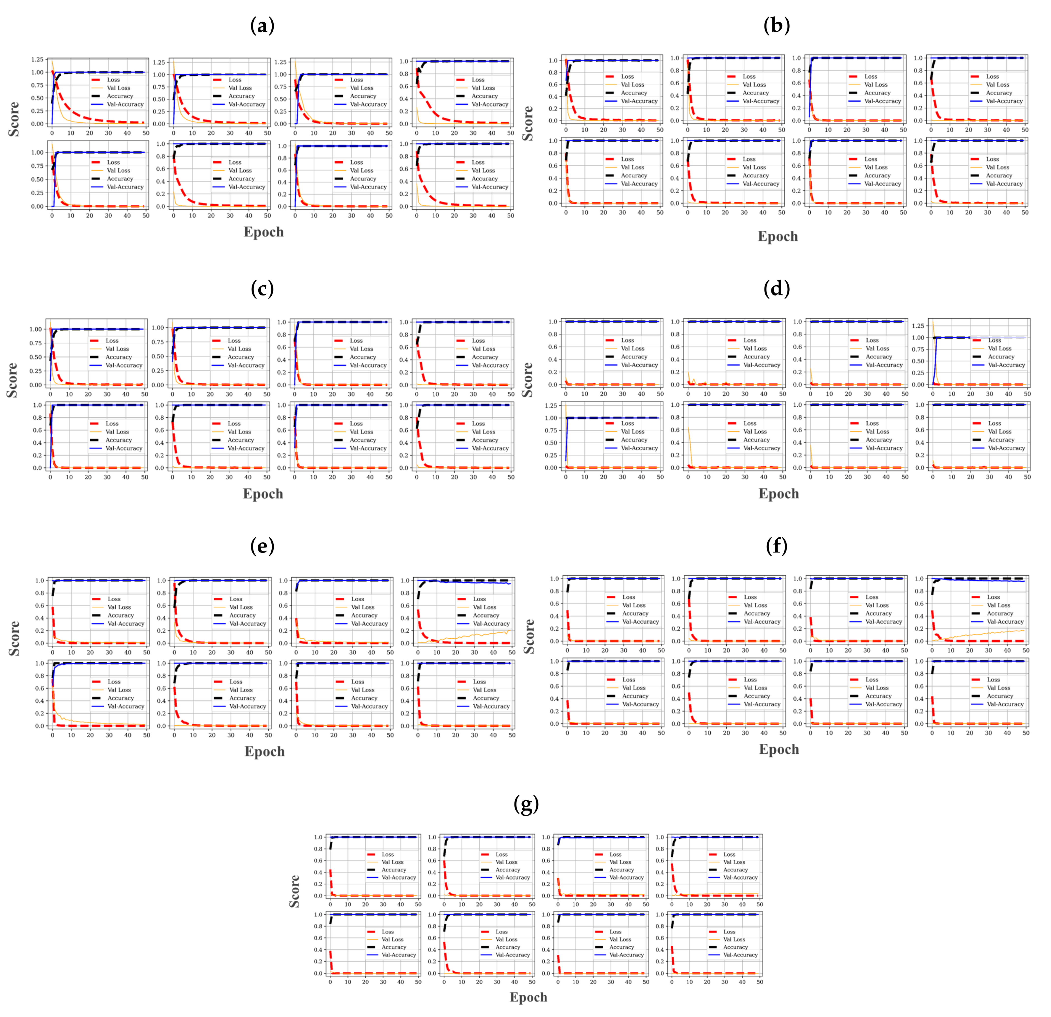
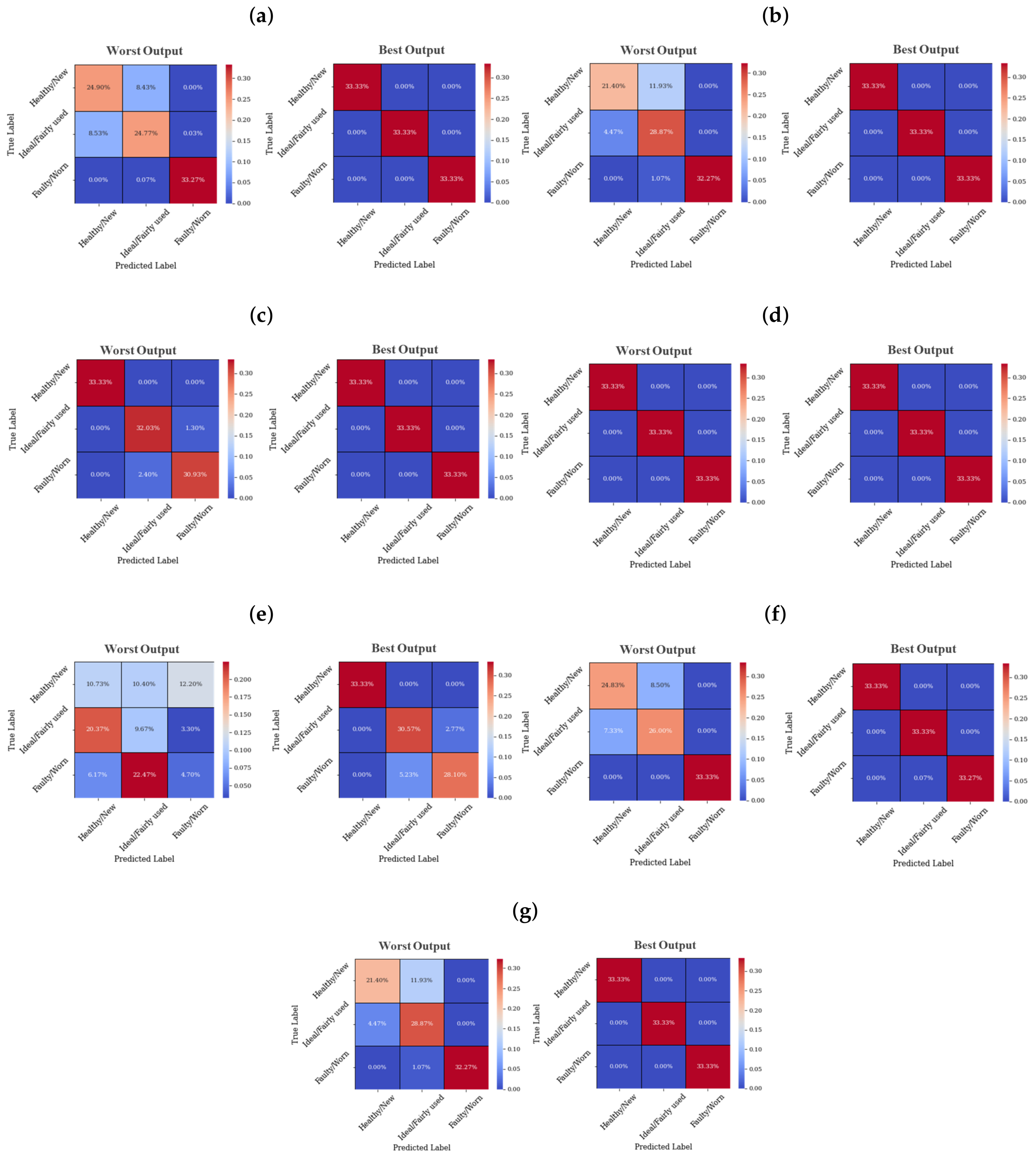
4.2. DL-Based Diagnostic Assessments

Apart from the spectral isolation module, the proposed intelligent monitoring framework features state-of-the-art stand-alone DL-based classifiers—1D-CNN and MLP. Although different custom and hybrid models have been reported in numerous works, generality remains a major concern for their global adoption [31]; therefore, it is often recommended to use established stand-alone DL-based models for practical cases. Although highly reliable, stand-alone DL algorithms have their limitations, which has motivated different methods for closing these limiting gaps. For example, CNNs are strongly affected by inputs with dynamic transient behavior, while MLPs are easily fooled by inputs due to their high dependence on a priori knowledge [32]. This is yet another valid rationale for adopting the spectral isolation technique as a preprocessing tool to ensure that only the critical spectral segments are retained.

Arguably, certain factors affect computational costs, transfer learning potentials of DL models between domains, model stochasticity and over-fitting, and they often include: the model’s structure—the number of layers, filters, and nodes in the mode—the right initialization method, choice of the activation function(s), hyperparameter values, learning rates and epoch sizes, the choice of regularization techniques employed, and the cost function (and the befitting loss minimization algorithm) employed. On the other hand, linear activation functions often flaw in comparison with nonlinear activation functions and even among the nonlinear counterparts, some are more suitable for classification problems (for example, ReLU and Softmax) while some are more suitable for regression problems (for example, ReLU, Tanh, and LeakyReLU). Consequently, it becomes a challenge to achieve a standard/global architecture for these models since, for instance, an excess of layers, nodes, and/or filters adversely effect computational efficiency and may lead to over-fitting, while the reverse may lead to under-fitting. However, users are motivated to try different architectures, and for each architecture, a cross-validation training/testing process over multiple trials is also encouraged to minimize the probability of accidental successes by the model(s). In this light, we designed different 1D-CNN and MLP models for the diagnostic process, and they are summarized in

Table 1. The different DNN models employed and their architectures.

Model	Architecture	Hyperparameters/Description
CNN64	Conv1D, GlobalAveragePooling1D, Dense_output	Filter1 = 64, kernel1_size = 3, activation_Conv1D = ReLU, activation_Dense_output = Softmax, optimizer = adam, Loss = categorical_crossentropy
CNN64_64	Conv1D—Conv1D, GlobalAveragePooling1D, Dense_output	Filter1 = Filter2 = 64, kernel1_size = 8, kernel2_size = 5, activation_Conv1D = ReLU, activation_Dense_output = Softmax, optimizer = adam, Loss = categorical_crossentropy
CNN64_Dense100	Conv1D, GlobalAveragePooling1D, Dense_100, Dense_output	Filter1 = 64, activation_Conv1D = ReLU, kernel1_size = 3, activation_Dense_100 = ReLU, activation_Dense_output = Softmax, optimizer = adam, Loss = categorical_crossentropy
FCN [33]	Conv1D+Batch_Norm, Conv1D+Batch_Norm, Conv1D+Batch_Norm, GlobalAveragePooling1D, Dense_output	Filter1 = 128, Filter2 = 256, Filter3 = 128, activation_Conv1D = ReLU, kernel1_size = 8, kernel2_size = 5, kernel3_size = 3, activation_Dense_output = Softmax, optimizer = adam, Loss = categorical_crossentropy
DNN64	Dense_64—Dense_output	MLP: nodes in Dense_64 = 64, activation_Dense_64 = ReLU, activation_Dense_output = Softmax, optimizer = adam, Loss = categorical_crossentropy
DNN128_64	Dense_128—Dense_64—Dense_output	MLP: nodes in Dense_128 = 128, nodes in Dense_64 = 64, activation_Dense_128 = activation_Dense_64 = ReLU, activation_Dense_output = Softmax, optimizer = adam, Loss = categorical_crossentropy
DNN100_150_50	Dense_100—Dense_150—Dense_50—Dense_output	MLP: nodes in Dense_100 = 100, nodes in Dense_150 = 150, nodes in Dense_50 = 50, activation_Dense_100 = activation_Dense_150 = activation_Dense_50 = ReLU, activation_Dense_output = Softmax, optimizer = adam, Loss = categorical_crossentropy

below.

As shown in Table 1, each of the DL models has different architectures with hyperparameter values that were chosen from experience (trial on different tasks), apart from the fully connected network (FCN) that was proposed in [33], and have been reported in many classification tasks. Overall, the Dense_output has three (3) nodes—one each for the different grinder wheel health stages, while the input shape is varied according to the shape (channel) of the input/source data. Generally, the “categorical_crossentopy” provides a reliable metric for evaluating the training loss for classification problems and was employed in all the models. On the other hand, the Adam weigh optimizer—an improved stochastic gradient descent-based optimizer—offers better efficiencies, faster convergence, and improved validation scores on large datasets and was used throughout.

The proposed diagnostic case study exploits vibration signals from seven (7) accelerometers with an optional module for employing the proposed spectral isolation technique; however, it also offers different input/source data channels, which may include the use of the raw signals (from all the accelerometers, the spindle only, or the frame only), the use of the critical segments from the signals (from all the accelerometers, the spindle only, or the frame only), and/or the use of alternating combinations of raw signals and critical segments from the signals (from all the accelerometers, the spindle only, or the frame only). For each of the models summarized in Table 1, each of the different input/source data channels were deployed for a training-validation process over a 5-fold cross-validation over 50 epochs on the training data (with 20% validation set included). Overall, eight (8) different input/source data channels were acquired, and they include raw spindle only ($S{P}_R$), critical spindle only ($S{P}_C$), raw frame only ($F{R}_R$), critical frame only ($S{P}_C$), raw spindle and raw frame ($SP\_F{R}_R$), critical spindle and raw frame ($SP\_F{R}_C$), raw spindle and critical frame ($S{P}_{R}F{R}_C$), and critical spindle and raw frame ($S{P}_{C}F{R}_R$). Figure 9 shows each of the models’ training history over the 50 epochs on the different input/source data channels.

As shown, the respective models have zero training and validation losses over the first few iterations (as shown in the red-dotted and yellow lines, respectively). These are also accompanied by a 100% training and validation accuracy from each of the models (as shown in the black-dotted and blue lines, respectively). These only validate that the models are quite efficient for learning the discriminative information stored in the training data and cannot form generalization criteria for assessing the models. Similarly, a test set was deployed for the models in an unsupervised manner, and their respective test scores were recorded.

Table 2. Test accuracy of DL models on different input/source data channels.

	Spindle Only		Frame Only		Spindle + Frame
Parameter	$S{P}_R$	$S{P}_C$	$F{R}_R$	$F{R}_C$	$SP\_F{R}_R$	$SP\_F{R}_C$	$S{P}_{R}F{R}_C$	$S{P}_{C}F{R}_R$
Dimension	($m\times n$) × 4	($m\times n$) × 4	($m\times n$) × 3	($m\times n$) × 3	($m\times n$) × 7	($m\times n$) × 7	($m\times n$) × 7	($m\times n$) × 7
CNN64	90.2%	97.8%	85.4%	88.9%	92.1%	98.0%	84.2%	88.3%
CNN64_64	92.1%	97.6%	88.1%	90.0%	92.5%	98.7%	88.9%	94.7%
CNN64_Dense100	93.6%	98.2%	88.6%	91.2%	92.2%	97.8%	90.1%	95.1%
FCN	96.0%	99.3%	91.1%	95.5%	95.7%	98.8%	92.3%	97.6%
DNN64	73.8%	85.6%	56.2%	75.8%	65.8%	87.2%	74.7%	83.7%
DNN128_64	88.7%	91.6%	82.6%	88.7%	90.3%	93.1%	90.6%	94.2%
DNN100_150_50	89.1%	92.1%	84.0%	90.1%	91.2%	94.0%	92.4%	93.0%

provides the dimensions of the different input/source data channels and the test scores of the different models, respectively.

Overall, the respective test accuracies of the models on the different input/source data channels are quite high; especially for the FCN whose architecture is the deepest of them all. A deeper analysis of the findings in Table 2 reveals a 4.6% and 7.5% improved diagnostic accuracy by the 1D-CNN and MLP models, respectively, between the use of the raw vibration signals and their critical segments. On the downside, the poor predictive accuracy of the more shallow models is shown by the DNN64’s low test accuracies (less than 88%) on all the input/source data channels. Amidst the predictive accuracies of the models across the rows, the positive impact of the proposed spectral isolation technique can be observed in the higher test accuracy between the use of raw signals and their critical segment counterparts; for instance, between $S{P}_R$ and $S{P}_C$, $F{R}_R$ and $F{R}_C$, and $SP\_F{R}_R$ and $SP\_F{R}_C$. Combining vibration measurements from the spindle can occur in four possible ways, which include: SP_FRR, $SP\_F{R}_C$, $S{P}_R\_F{R}_C$, and $S{P}_C\_F{R}_R$. These different combinations produce different diagnostic accuracies, as shown in Table 2. However, a significant observation is that for the respective DL models, using the critical segments from both vibration sources (frame and spindle—$SP\_F{R}_R$) produces better diagnostic accuracies in comparison with the other spindle-frame combinations—$SP\_F{R}_R$, $S{P}_R\_F{R}_C$, and $S{P}_C\_F{R}_R$. Nonetheless, the test accuracies from each Of the DL models were highest when only spindle vibrations were used (raw and critical segments).

Interestingly, between the 1D-CNN and MLP variants presented, it can be observed that the 1D-CNN has superior classification efficiencies even with a shallow architecture, such as the CNN64. This is attributed to the filters that scan through the signals for discriminative features, and with the $GlobalAveragePooling1D$ integrated in their architecture, the 1D-CNN models are better able to prioritize the maximum value for feature values of a feature matrix and uses it to create a down-sampled (pooled) feature matrix. This strongly provides valid support for choosing the 1D-CNN models over the MLP models.

Although the test accuracy provides a global perspective for performance evaluation of the models, it may be more important to assess their class-specific (the different health stages of the wheels) performance to better ascertain their probability for false/positive predictions. Generally, the confusion matrix provides a reliable avenue for such assessments and was employed. For each of the input/source data channels, the confusion matrix of the models was computed, and, overall, there were 56 different outputs, most of which returned a perfect prediction for the different classes, while a few imperfect predictions were also returned. Because it would be futile to present all the 56 matrices in this study (in addition to the numerous similarities in the models’ outputs), we have provided, in Figure 10, each model’s best and worst confusion matrix outputs and their corresponding inferences that can be drawn from them.

As shown in the maximum true positives in Figure 10d, it can be observed that the FCN is the most accurate of all the models, followed by the $CNN64\_Dense100$ in Figure 10c, whose worst prediction was recorded for the $F{R}_R$ data source. As the CNN models become more shallow ($CNN64$ and $CNN64\_64$), the false alarm rate of predictions becomes higher, as observed in the false positives and false negatives in Figure 10a,b. Although the best outputs for the $CNN64$ and $CNN64\_64$ models are perfect, such as the FCN, the reduced true positives in their worst outputs, as shown in Figure 10a,b, only reflect on the inherent deficiencies of shallow CNN models, especially for inputs with very small discriminance in the inputs, such as the $F{R}_R$. In contrast, the $S{P}_C$, $F{R}_C$, $SP\_F{R}_C$, which, respectively, are critical segments from the raw signals, offer inputs that are more discriminative for improved diagnostic results. Overall, most of the best outputs presented in Figure 10 were produced for the inputs $S{P}_C$, $F{R}_C$, $SP\_F{R}_C$, while the worst outputs were produced for $F{R}_R$, which generally hints not only at the importance of the spectral isolation but also the limited efficiencies of monitoring the component via the frame only. While the sensors under the spindle provide more resourceful information for monitoring, the sensors on the frame provide supplementary information for a more comprehensive monitoring process and are recommended (even though the overall accuracy of using the spindle only is marginally higher).

Although the results in Table 2 and Figure 10 support the use of the FCN model for accurate monitoring, it is also important to assess the computational cost implications of using the models. This offers another avenue for a more informed decision-making criteria for diagnostic modeling. In view of this, we conducted a computational cost assessment on the models, and it is presented in Figure 11.

The values shown in Figure 11 above are the times (in minutes) for the training-testing process of each DL model on the respective input/source data channels. The hardware specifications for the computer used in the analyses is: AMD Ryzen 7 (manufactured in Taiwan), 2700 Eight-core 3.20 GHz processor, and 16 GB RAM, while the analyses were performed using Keras—a Python-based DL library. As shown, the computational costs of using the FCN are at least three to four times higher than using the other models. This may be a major concern for cases where computational resources are a major decision-making criteria; however, since most state-of-the-art computers often feature high-end processing units, computational costs may not be a major concern. On the other hand, choosing a more shallow DL model architecture offers better computational efficiencies, as shown in the low computational costs associated with the DL models (except the FCN). From this perspective, one may be inclined to find an optimal balance between computational accuracy and computational costs, which realistically offers a better decision-making rationale. In that case, the 1D-CNN models—$CNN64$, $CNN64$, and $CNN64\_64$—offer realistic alternatives to the FCN since they offer high test accuracies (as shown in Table 2), minimal false alarm rates (as shown in Figure 10a–c), and comparatively lower computational cost than the FCN. Moreover, the cost implications of combining both vibration sources are shown in Figure 11, whereby using the raw signals from both sources ($SP\_F{R}_R$) is more computationally expensive (13.71 min) than when the other combinations were employed—13.4 min for $SP\_F{R}_C$, 13.13 min for $S{P}_R\_F{R}_C$, and 12.58 min for $S{P}_C\_F{R}_R$. Overall, the study reveals an improved diagnostic accuracy by the 1D-CNN and DNN models of about 1.3% and 5.71% reduced computational costs.

5. Conclusions and Future Works

In this study, a vibration-based multi-sensor intelligent wear monitoring framework is proposed to solve the compound health diagnosis of high-frequency micro drill bit ARIS using spectral isolation and deep learning models. Because DL models are popular for disparaging the hectic (and less efficient) process of manual hand-crafted feature extraction process with automated (and more reliable) efficiencies, we exploited the 1D-CNN and MLP models on the vibration signals acquired from the frame and spindle of the regrinding unit of a micro drill bit ARIS (model TGM-1011) for monitoring the wear severity of the grinding wheel. A major contribution of the study is the spectral isolation module, which helps prioritize only the critical spectral segments of the vibration signals via an FFT-based signal processing technique for improved monitoring accuracies at reduced computational costs.

Results from deploying the DL models on the different input/source data channels—raw and critical segments—of the signals reveal 4.6% and 7.5% improved diagnostic accuracy by the 1D-CNNs and MLP s, respectively, at about 1.3% and 5.71% reduced computational costs, respectively. Moreover, the study shows that as the models become more shallow, the false alarm rate of predictions becomes higher; especially when using the raw vibration signals. While the sensors under the spindle provide more resourceful information for monitoring, the sensors on the frame provide supplementary information for a more comprehensive monitoring process and are recommended (even though the overall accuracy of using the spindle only is marginally higher). On the extreme side, the study reveals that using very deep models, such as the FCN, comes with significant computational costs regardless of the data sources employed and should be considered for cases where computational resources are a major decision-making factor. While a more shallow model (in comparison with the FCN) offers better computational efficiencies, its optimal use may rely on the proposed spectral isolation module to minimize the probability of false predictions.

While the findings validate the efficiencies of the proposed monitoring framework, the inherent issues of optimal sensor selection still pose a significant concern because accelerometers may not be the most appropriate for the equipment. No doubt, alternative sensors, such as acoustic emission sensors and cameras, may offer better monitoring solutions, either as stand-alone or hybrid sensing mechanisms. Although our choice of accelerometers was fundamentally motivated by their strong magnetic properties, cost efficiency, sensor localization efficiencies, and the comprehensive monitoring opportunities offered by combining the measurements from the spindle and frame (which, by the way, are major advantages over the alternative sensing methods since the regrinding is always in motion), we believe accelerometers only provide inferred knowledge of the regrinding unit as mechanical responses (which may be compromised by other unrecognizable sources). The authors agree that the use of indirect monitoring methods, such as vibration sensors, may not be as efficient as direct monitoring methods. However, our research offers significant success in the proposed case study, which unfortunately has not been studied in the past. We believe our study provides a strong paradigm for bench-marking our continued research in the case study as we continue to investigate other sensing methods for improved health monitoring.

On the flip side, we believe cameras are more befitting since they can better provide direct information on the grinding wheels’ health states for a more accurate wear monitoring. However, its real-time usability may be affected since the wheels rotate at high speeds and may produce unclear images in real-time. Further, finding an optimal camera localization point is another major challenge. These lapses present opportunities for continued research in the domain and have motivated our continued research.

References

1. Thomas, D. The Costs and Benefits of Advanced Maintenance in Manufacturing; Advanced Manufacturing Series (NIST AMS); National Institute of Standards and Technology: Gaithersburg, MD, USA, 2018. [CrossRef]
2. Abidi, M.H.; Mohammed, M.K.; Alkhalefah, H. Predictive Maintenance Planning for Industry 4.0 Using Machine Learning for Sustainable Manufacturing. Sustainability 2022, 14, 3387. [Google Scholar] [CrossRef]
3. Zhao, J.; Gao, C.; Tang, T. A Review of Sustainable Maintenance Strategies for Single Component and Multicomponent Equipment. Sustainability 2022, 14, 2992. [Google Scholar] [CrossRef]
4. Yin, S.; Rodríguez-Andina, J.; Jiang, Y. Real-Time Monitoring and Control of Industrial Cyberphysical Systems: With Integrated Plant-Wide Monitoring and Control Framework. IEEE Ind. Electron. Mag. 2019, 13, 38–47. [Google Scholar] [CrossRef]
5. Akpudo, U.E.; Hur, J.-W. D-dCNN: A Novel Hybrid Deep Learning-Based Tool for Vibration-Based Diagnostics. Energies 2021, 14, 5286. [Google Scholar] [CrossRef]
6. Huang, B.-W.; Tseng, J.-G. Drilling Vibration in a micro drilling Process Using a Gas Bearing Spindle. Adv. Mech. Eng. 2020. [Google Scholar] [CrossRef]
7. Lee, C.-H.; Jwo, J.-S.; Hsieh, H.-Y.; Lin, C.-S. An Intelligent System for Grinding Wheel Condition Monitoring Based on Machining Sound and Deep Learning. IEEE Access 2020, 8, 58279–58289. [Google Scholar] [CrossRef]
8. Jia, F.; Lei, Y.; Lin, J.; Zhou, X.; Lu, N. Deep neural networks: A promising tool for fault characteristic mining and intelligent diagnosis of rotating machinery with massive data. Mech. Syst. Signal Process. 2016, 72, 303–315. [Google Scholar] [CrossRef]
9. Stavropoulos, P.; Papacharalampopoulos, A.; Vasiliadis, E.; Chryssolouris, G. Tool wear predictability estimation in milling based on multi- sensorial data. Int. J. Adv. Manuf. Technol. 2016, 82, 509–521. [Google Scholar] [CrossRef] [Green Version]
10. Akpudo, U.E.; Hur, J.-W. Investigating the Efficiencies of Fusion Algorithms for Accurate Equipment Monitoring and Prognostics. Energies 2022, 15, 2204. [Google Scholar] [CrossRef]
11. Kim, S.; Akpudo, U.E.; Hur, J.-W. A Cost-Aware DNN-Based FDI Technology for Solenoid Pumps. Electronics 2021, 10, 2323. [Google Scholar] [CrossRef]
12. Lee, N.; Azarian, M.H.; Pecht, M.G. An Explainable Deep Learning-based Prognostic Model for Rotating Machinery. arXiv 2020, arXiv:2004.13608. [Google Scholar]
13. Jianyu, L.; Yibin, C.; Zhe, Y.; Yunwei, H.; Chuan, L. A novel self-training semi-supervised deep learning approach for machinery fault diagnosis. Int. J. Prod. Res. 2022. [Google Scholar] [CrossRef]
14. Yu, X.; Zhao, Y.; Gao, Y.; Xiong, S. MaskCOV: A random mask covariance network for ultra-fine-grained visual categorization. Pattern Recognit. 2021, 119, 108067. [Google Scholar] [CrossRef]
15. Watson, M.; Sheldon, J.; Amin, S.; Lee, H.; Byington, C.; Begin, M. A Comprehensive High Frequency Vibration Monitoring System for Incipient Fault Detection and Isolation of Gears, Bearings and Shafts/Couplings in Turbine Engines and Accessories. In Proceedings of the ASME Turbo Expo 2007: Power for Land, Sea, and Air, Montral, QC, Canada, 14–17 March 2007; pp. 885–894. [Google Scholar] [CrossRef]
16. Marple, L. Computing the discrete-time ‘analytic’ signal via FFT. IEEE Trans. Signal Process 1999, 47, 2600–2603. [Google Scholar] [CrossRef]
17. Ulsoy, A.G.; Tekinalp, O.; Lenz, E. Dynamic modeling of transverse drill bit vibrations. CIRP Ann. 1984, 33, 253–258. [Google Scholar] [CrossRef]
18. Fuji, H.; Marui, E.; Ema, S. Whirling vibration in drilling part 3: Vibration analysis in drilling workpiece with a pilot hole. J. Eng. Ind. 1988, 110, 315–321. [Google Scholar] [CrossRef]
19. Kuk, Y.H.; Park, S.R.; Park, K.J.; Choi, H.J. A Study on Process Simulation Analysis of the Water Jet Cleaning Robot System for Micro Drill-bits. Soc. Comput. Des. Eng. 2015, 20, 291–297. [Google Scholar]
20. Akpudo, U.; Jang-Wook, H. A Multi-Domain Diagnostics Approach for Solenoid Pumps Based on Discriminative Features. IEEE Access 2020, 8, 175020–175034. [Google Scholar] [CrossRef]
21. Medrano, R.; Aznarte, J.L. A spatio-temporal attention-based spot-forecasting framework for urban traffic prediction. Appl. Soft Comput. 2020, 96, 106615. [Google Scholar] [CrossRef]
22. Kim, H.; Lee, W.; Kim, M.; Moon, Y.; Lee, T.; Cho, M.; Mun, D. Deep-learning-based recognition of symbols and texts at an industrially applicable level from images of high-density piping and instrumentation diagrams. Expert Syst. Appl. 2021, 183, 115337. [Google Scholar] [CrossRef]
23. Cabaneros, S.M.; Calautit, J.K.; Hughes, R. A review of artificial neural network models for ambient air pollution prediction. Environ. Model. Softw. 2019, 119, 285–304. [Google Scholar] [CrossRef]
24. Ahishakiye, E.; Bastiaan, M.B.; Tumwiine, J.; Wario, R.; Obungoloch, J. A survey on deep learning in medical image reconstruction. Intell. Med. 2021, 1, 118–127. [Google Scholar] [CrossRef]
25. Weigold, M.; Ranzau, H.; Schaumann, S.; Kohne, T.; Panten, N.; Abele, E. Method for the application of deep reinforcement learning for optimised control of industrial energy supply systems by the example of a central cooling system. CIRP Ann. 2021, 70, 17–20. [Google Scholar] [CrossRef]
26. Sharma, O. Deep Challenges Associated with Deep Learning. In Proceedings of the 2019 International Conference on Machine Learning, Big Data, Cloud and Parallel Computing (COMITCon), Faridabad, India, 14–16 February 2019; pp. 72–75. [Google Scholar] [CrossRef]
27. Kim, S.; Han, G. 1D CNN Based Human Respiration Pattern Recognition using Ultra Wideband Radar. In Proceedings of the 2019 International Conference on Artificial Intelligence in Information and Communication (ICAIIC), Okinawa, Japan, 11–13 February 2019; pp. 411–414. [Google Scholar] [CrossRef]
28. Bircanoğlu, C.; Arıca, N. A comparison of activation functions in artificial neural networks. In Proceedings of the 2018 26th Signal Processing and Communications Applications Conference (SIU), Izmir, Turkey, 2–5 May 2018; pp. 1–4. [Google Scholar] [CrossRef]
29. Kingma, D.P.; Ba, J. Adam: A Method for Stochastic Optimization. arxiv 2015, arXiv:1412.6980v9. [Google Scholar]
30. Lai, K.K.; Mishra, S.K.; Ram, B. On q-Quasi-Newton’s Method for Unconstrained Multiobjective Optimization Problems. Mathematics 2020, 8, 616. [Google Scholar] [CrossRef] [Green Version]
31. Li, J.; Shen, C.; Kong, L.; Wang, D.; Xia, M.; Zhu, Z. A New Adversarial Domain Generalization Network Based on Class Boundary Feature Detection for Bearing Fault Diagnosis. IEEE Trans. Instrum. Meas. 2022, 71, 1–9. [Google Scholar] [CrossRef]
32. Jirak, D.; Wermter, S. Potentials and Limitations of Deep Neural Networks for Cognitive Robots. arXiv 2018, arXiv:1805.00777. [Google Scholar]
33. Wang, Z.; Yan, W.; Oates, T. Time series classification from scratch with deep neural networks: A strong baseline. arXiv 2016, arXiv:1611.06455. [Google Scholar]
Figure 1. CAD plan view of the G50150 micro drill bit ARIS highlighting the collet and regrinding unit.
Algorithms 15 00194 g001
Figure 2. Proposed monitoring framework.
Algorithms 15 00194 g002
Figure 3. A picture of the micro drill bit ARIS (model TGM-1011) with the sensor locations and data acquisition system.
Algorithms 15 00194 g003
Figure 4. Pictures of the grinding wheel at (a) healthy/normal state, (b) fairly used state—about 40–50% life remaining useful, and (c) faulty state—about 0–10% life remaining useful.
Algorithms 15 00194 g004
Figure 5. Raw vibration signals for (a) spindle at healthy/normal state, (b) spindle at fairly used state, (c) spindle at faulty state, (d) frame at healthy/normal state, (e) frame at fairly used state, and (f) frame at faulty state.
Algorithms 15 00194 g005
Figure 6. Spectral comparison of different grinder health states. (a) Spindle, (b) frame.
Algorithms 15 00194 g006
Figure 7. Spectral comparison of different grinder health states. (a) Spindle (critical segment), (b) frame (critical segment).
Algorithms 15 00194 g007
Figure 8. Raw vibration signals (in blue) and their corresponding spectral isolation outputs (in red) for (a) spindle at healthy/normal state, (b) spindle at fairly used state, (c) spindle at faulty state, (d) frame at healthy/normal state, (e) frame at fairly used state, and (f) frame at faulty state.
Algorithms 15 00194 g008
Figure 9. Training history for (a) CNN64, (b) CNN64_64, (c) CNN64_Dense100, (d) FCN, (e) DNN64, (f) DNN128_64, and (g) DNN100_150_50. For each subfigure, the eight images respectively represent the training histories for the eight different input/source data channels in the order: S P R , S P C , F R R , S P C , S P _ F R R , S P _ F R C , S P R F R C , S P C F R R .
Algorithms 15 00194 g009
Figure 10. Worst and best Confusion matrices produced by the DL models (a) C N N 64 , (b) CNN64_64, (c) CNN64_Dense100, (d) FCN, (e) DNN64, (f) DNN128_64, and (g) DNN100_150_50.
Algorithms 15 00194 g010
Figure 11. Computational cost assessment of the DL models on the different input/source data channels. The green bars (Avg cost) are the mean value of the computational costs of the DL models per input/source data channel.
Algorithms 15 00194 g011