Constructing the Neighborhood Structure of VNS Based on Binomial Distribution for Solving QUBO Problems

Abstract

The quadratic unconstrained binary optimization (QUBO) problem is categorized as an NP-hard combinatorial optimization problem. The variable neighborhood search (VNS) algorithm is one of the leading algorithms used to solve QUBO problems. As neighborhood structure change is the central concept in the VNS algorithm, the design of the neighborhood structure is crucial. This paper presents a modified VNS algorithm called “B-VNS”, which can be used to solve QUBO problems. A binomial trial was used to construct the neighborhood structure, and this was used with the aim of reducing computation time. The B-VNS and VNS algorithms were tested on standard QUBO problems from Glover and Beasley, on standard max-cut problems from Helmberg–Rendl, and on those proposed by Burer, Monteiro, and Zhang. Finally, Mann–Whitney tests were conducted using $\alpha =0.05$, to statistically compare the performance of the two algorithms. It was shown that the B-VNS and VNS algorithms are able to provide good solutions, but the B-VNS algorithm runs substantially faster. Furthermore, the B-VNS algorithm performed the best in all of the max-cut problems, regardless of problem size, and it performed the best in QUBO problems, with sizes less than 500. The results suggest that the use of binomial distribution, to construct the neighborhood structure, has the potential for further development.

1. Introduction

Combinatorial optimization has attracted a good deal of attention, as it has many applications in various fields [1]. However, it is not always easy to solve combinatorial optimization problems, especially in some cases, classified as NP-hard problems. In this kind of situation, the use of the approximation method is a reasonable option [2]. One of the approximation methods that has attracted a great deal of attention in modern optimization is the metaheuristic method [3], which is designed to obtain good solutions within a reasonable time frame [4]. Even though it is not easy to prove that a solution obtained using the metaheuristic method is a global optimum [5], the results are, often, very close to the global optimum.

Depending on the case, a combinatorial problem can be formulated in various ways, so that it can be be easily solved. One method is the use of a Boolean or binary vector, which, despite its simplicity, is a compelling method for solving many combinatorial problems. A specific binary formulation forms a major optimization problem category, called “quadratic unconstrained binary optimization (QUBO)”, or “Ising model optimization” in some of the literature [6]. In the QUBO problem, given $\mathit{Q}=\left(q_{ij}\right)$ is a symmetric n-square matrix of coefficients, the objective is to maximize the function:

$$f\left(\mathit{X}\right)={\mathit{X}}^{\mathit{T}}\mathit{QX}=\sum _{i=1}^n\sum _{j=1}^n{q}_{ij}{x}_i{x}_j$$

(1)

where $\mathit{X}=\left(x_i\right)$ is an n-dimensional vector of binary variables, i.e., $x_i\in \{0,1\}$ for $i=1,2,...,n$. QUBO problems are categorized as NP-hard problems [7], and their decision form is NP-complete [6]. The implementation of the QUBO formulation can be found in many combinatorial problems, e.g., graph coloring, partition, and maximum cut (max-cut) [6], which were included in Karp’s original 21 NP-complete problems [8]. More applications of QUBO were described by Glover and Kochenberger [9].

It is as difficult to solve QUBO problems as it is to solve other NP-hard problems. Many metaheuristic algorithms have been devised to solve them, based on the requirement that they are solved within a reasonable amount of time. Examples of these are simulated annealing [10], tabu search [11], genetic algorithm [12], and local search [13] algorithms. One particular metaheuristic algorithm that uses local search is the variable neighborhood search (VNS) algorithm [14]. The VNS algorithm can solve various problems, including QUBO problems.

As a single-trajectory-based algorithm, the VNS algorithm has the advantage that it is resource-efficient. Furthermore, its memory requirements are relatively low, compared to population-based metaheuristic algorithms. Therefore, the VNS algorithm is suitable for use in solving large-scale problems and does not need large memory allocations. It is a simple concept, and the VNS algorithm is, often, used in its original form, a modified form, or hybridized with another algorithm [15,16].

The VNS algorithm has been shown to perform well in various problems. Its applications include the max-cut combinatorial problem [17,18], the scheduling problem [19,20], the layouting problem [21], the vehicle routing problem [22], and the multiprocessor scheduling problem with communication delays [23]. It has, also, been used to tune proportional–integral–derivative controllers in cyber–physical systems [24]. Not only has the VNS algorithm been applied in numerous ways, but it has, also, been, often, used in combination with other algorithms to obtain combined performance. It is possible to hybridize the VNS algorithm with other metaheuristic algorithms, such as with the genetic algorithm [25], the particle swarm optimization algorithm [26], the migrating birds optimization algorithm [27], and the simulated annealing algorithm [28]. The VNS algorithm can also be implemented in parallel programming, by using a graphical processing unit [29] to leverage its performance.

Many factors determine the performance of the VNS algorithm, i.e., the initialization method, neighborhood structure construction, local search procedures, and update mechanisms. Although there are many determining factors, neighborhood structure is the central concept of the VNS algorithm that significantly influences its performance. One version of the VNS algorithm is based on the dynamic neighborhood model, proposed by Mladenović and Hansen [14]. Changing the neighborhood structure during a search enables the algorithm to escape the local optimum trap [30], as it allows the algorithm to move from one basin of search to another. The construction of a neighborhood is, thus, crucial to the performance of the VNS algorithm. However, in terms of solving the QUBO problem, previous research reports regarding neighborhood construction are difficult to find. The Hamming distance is commonly used in the basic VNS algorithm to construct the neighborhood, when solving a QUBO problem [5,17,31].

The VNS algorithm uses a strictly monotonic increasing neighborhood structure, when the local search does not yield a better solution. As a result, the basic VNS algorithm takes quite a long time to yield a good solution. A new version called “Jump VNS” was introduced, to speed up the neighborhood construction process. It enables the neighborhood structure to leap ahead, in accordance with parameter $k_{step}\in \mathbb{N}$ [32]. The basic VNS algorithm, which does not have the jump ability, is obtained by setting $k_{step}=1$. The performance of the Jump VNS algorithm does not appear to have been previously reported.

The VNS algorithm is simple, and the ability to slowly change the neighborhood structure is an advantage of its use. However, this is, also, a weakness of the VNS algorithm. This gradual but slow change may impact the length of computation time. Although it may be sped up with Jump VNS, the thorough search behavior may be lost. For example, setting the maximum distance on a VNS algorithm to 100 results in 100 times neighborhood-structure change, at most, but setting $k_{step}=2$ on Jump VNS results in only 50 times neighborhood structure change. This value is even less if a larger $k_{step}$ is used. So, the VNS and Jump VNS algorithms are not flexible.

This paper elaborates on the basic VNS algorithm and introduces a new method of improving it by focusing on the neighborhood structure by implementing binomial distribution. Instead of a strictly monotonic increase in neighborhood structure, the neighborhood distance follows a binomial distribution. Although the binomial distribution will cause a non-monotonic increase, the trend of a widening structure will remain the same. We investigated the potential of our proposed algorithm to be used in some QUBO and max-cut problems.

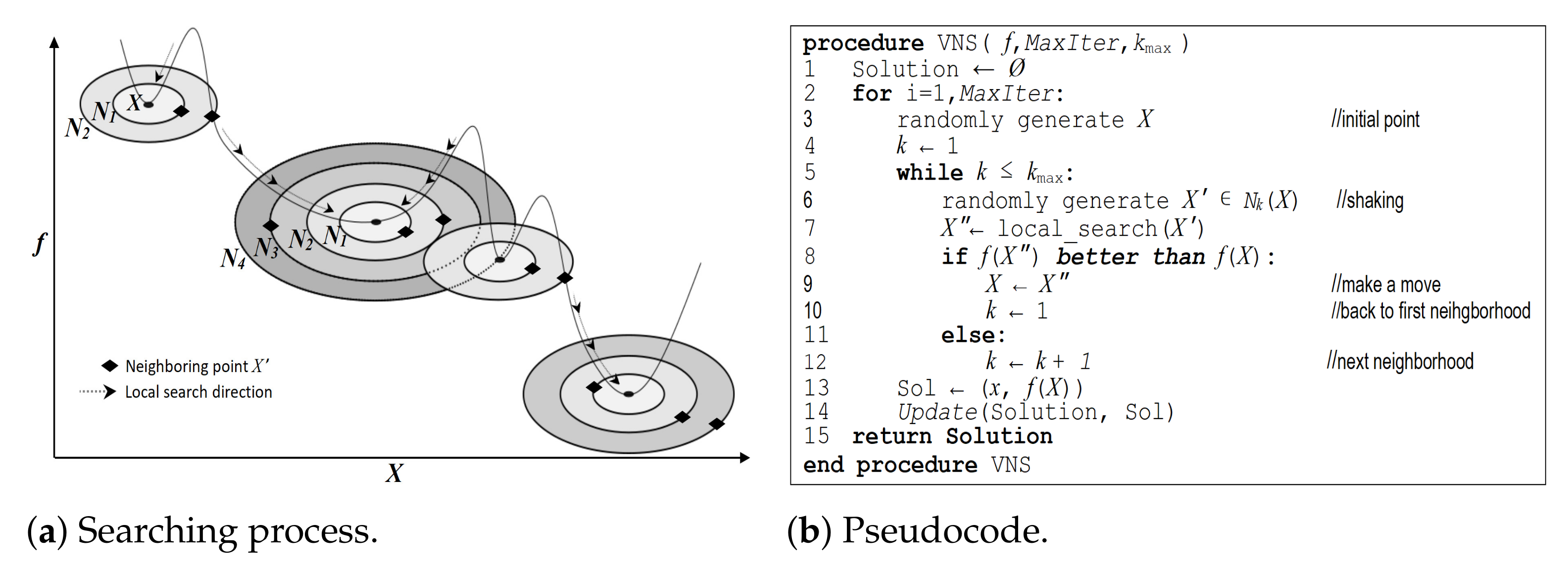
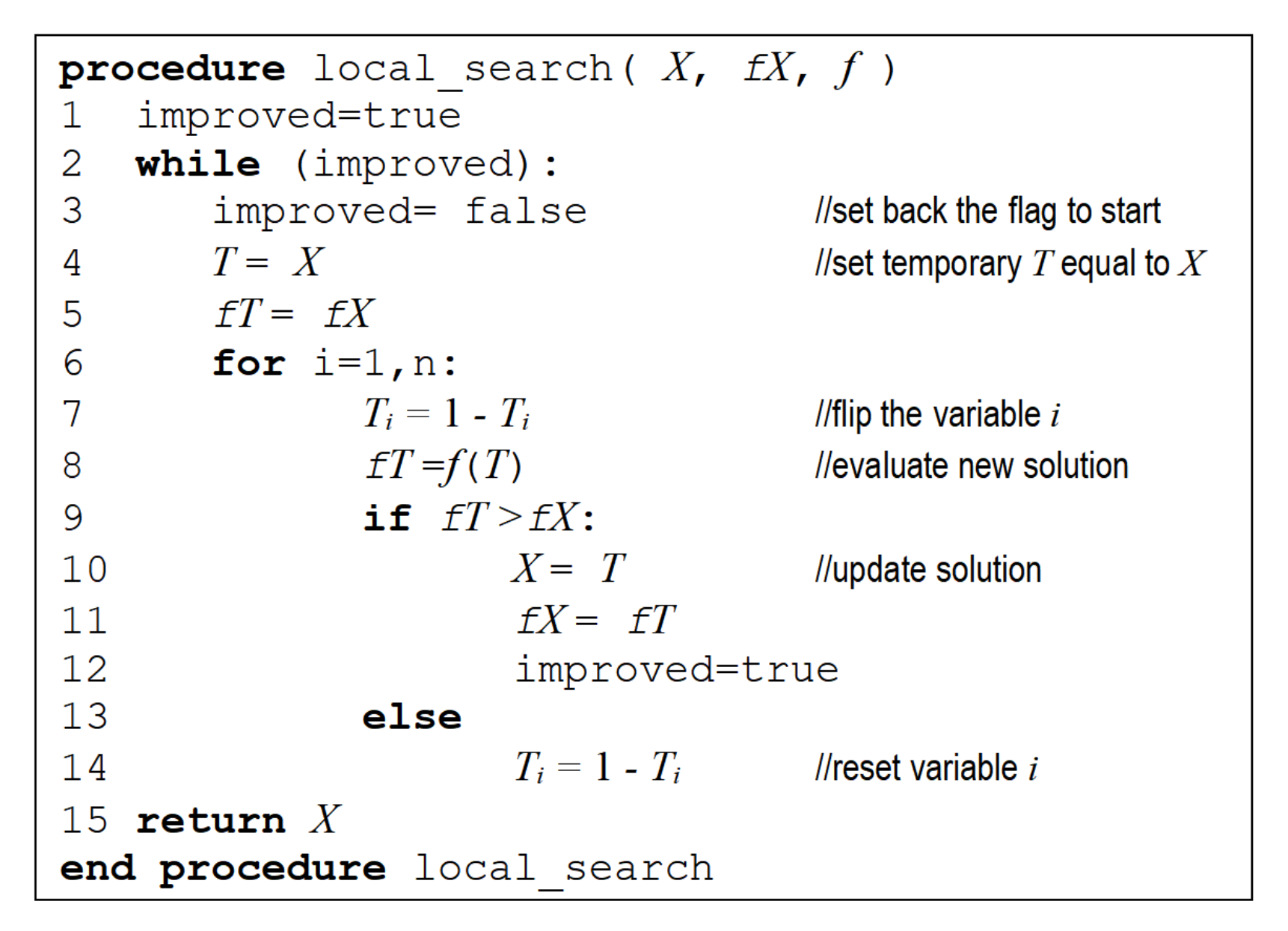
2. VNS Algorithm

The VNS algorithm is a well-known metaheuristic algorithm that utilizes dynamic neighborhood structure changes. The simple implementation of the VNS algorithm starts from a non-deterministic guest initial point and, then, attempts refinements using a local search. The algorithm shifts from its initial point to a neighboring point, before a local search is carried out. The algorithm should move to another neighborhood structure, when the local search does not yield a better solution. The algorithm systematically exploits the following observations [33]:

• Observation 1: A local minimum for one neighborhood structure is not necessarily so for another;
• Observation 2: A global minimum is a local minimum for all of the possible neighborhood structures;
• Observation 3: For many problems, local minimums for one or several neighborhoods are relatively similar to each other.

In other words, according to observation 1, a local minimum for a specific neighborhood structure is not necessarily a local minimum for other neighborhood structures. Other neighborhoods may have other local optimums. The second observation means that the global minimum will only be found after examining all of the possible local optimums, which requires the examination of all of the possible neighborhood structures. Other neighborhoods should be examined, if a local minimum is not the global minimum. The last observation is an empirical observation that suggests a local optimum, usually, provides information that helps determine the global optimum [33]. For example, in the case of a multi-variable function, several variables, often, have the same value in the local optimum as in the global optimum [33].

There are several versions of the VNS algorithm; the most prominent is the dynamic neighborhood model, proposed by Mladenović and Hansen [14]. They proposed a random shift to a neighboring point ${\mathit{X}}^{\prime }$, which would be used instead of the initial point $\mathit{X}$, as the base point of a local search. They called this shifting “shaking”. In this model, if the local search does not yield an improvement, the neighborhood structure is expanded. This change enables the algorithm to move to another basin to be exploited. To retain efficiency, the change must be limited by a parameter that defines the maximum number of neighborhood structures examined. If the local search yields an improvement, the structure is, suddenly, shrunk back to the first structure. The use of this clever expand-and-shrink neighborhood structure, during a search, enables the VNS algorithm to avoid the local optimum trap [30] because the algorithm moves from one basin to another. Figure 1a shows the searching process [32] in the context of minimization. The pseudocode of the VNS algorithm is shown in Figure 1b.

A change in neighborhood structure can be illustrated as an expanded disc, with point $\mathit{X}$ at the center. The neighborhood structure expands, following variable $k\in \mathbb{N}$. As proposed elsewhere [17,31,34], neighborhood structure N is associated with variable k, which is limited by parameter $k_{max}\in \mathbb{N}$. Thus, Hamming distance d increases, following k, when solving QUBO problems. Accordingly, a point ${\mathit{X}}^{\prime }\in N_k\left(\mathit{X}\right)$ means that the Hamming distance $d({\mathit{X}}^{\prime },\mathit{X})=\left|{\mathit{X}}^{\prime }-\mathit{X}\right|$ is exactly k. This neighborhood structure is the standard that is used in solving QUBO problems. The neighborhood structure of the basic VNS algorithm for use in solving QUBO problems is formulated as

$$N_k\left(\mathit{X}\right)=\{\mathit{Y}:|\mathit{Y}-\mathit{X}|=k\},$$

(2)

for $k=1,2,...,k_{max}$.

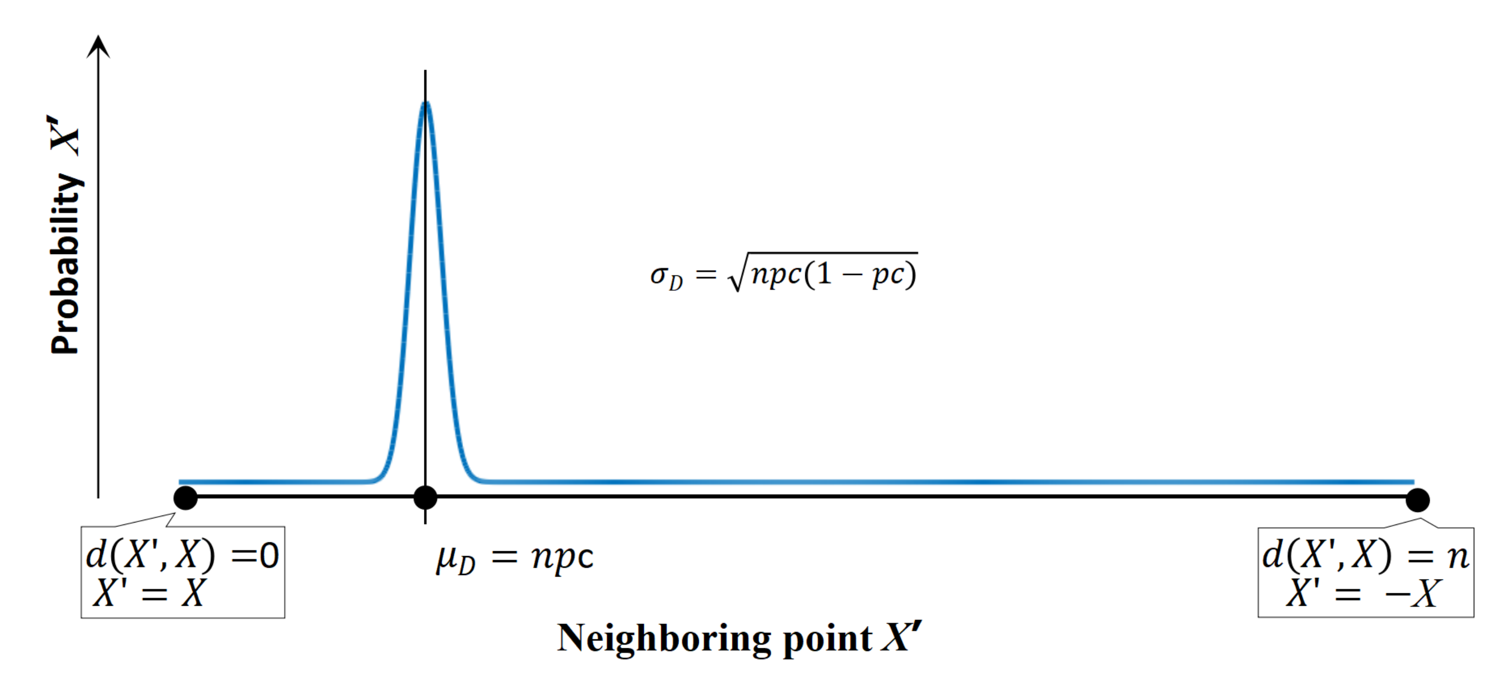
3. Proposed Neighborhood Structure

The strictly monotonic expanding neighborhood structure used in the VNS algorithm is tenable. However, there is no guarantee that this expansion type will always result in a better solution. To exploit this technique to solve any QUBO problem, we propose the use of binomial distribution to create a neighborhood structure. As the proposed algorithm is based on the VNS algorithm, it takes advantage of the characteristics of the VNS algorithm, while aiming to reduce the computation time required.

Our proposed structure enables the algorithm to expand the neighborhood, by following a random schema. However, it is good to maintain a gradual expansion trend. In the basic VNS algorithm, the neighboring point ${\mathit{X}}^{\prime }\in N_k\left(\mathit{X}\right)$ is obtained by flipping k numbers of the element of $\mathit{X}$. The flipped elements are chosen randomly. As a result, some elements are changed, from 1 to 0 or vice versa, while some remain. Instead of applying this basic neighborhood structure, we propose a mechanism of determining whether each element should be flipped or not. Each element will be flipped, by considering a flip probability. The proposed neighborhood structure is as follows: we define a trial T, to flip each element of a vector $\mathit{X}=(x_1,x_2,...,x_n)$, to obtain ${\mathit{X}}^{\prime }=(x_1^{\prime },x_2^{\prime },...,x_n^{\prime })\in N\left(\mathit{X}\right)$, in accordance with the following rule:

$$x_i^{\prime }=\left\{\begin{array}{ll}flip\left(x_i\right)& ,\mathrm{with}\mathrm{probability}p\in [0,1]\hfill \\ x_i\hfill & ,\mathrm{with}\mathrm{probability}(1-p)\hfill \end{array}\right.,$$

(3)

where

$$flip\left(x_i\right)=\left\{\begin{array}{cc}1-x_i\hfill & ,\mathrm{for}\{0,1\}\mathrm{encode}\hfill \\ -x_i\hfill & ,\mathrm{for}\pm 1\mathrm{encode}\hfill \end{array}\right..$$

(4)

This trial satisfies binomial requirements, as it is repeated n times, where n corresponds to the vector length and sets a fixed probability p. Suppose a random variable A represents the number of flipped elements, and let a random variable D represent the obtained Hamming distance d. Then, there is a clear correspondence between random variable A and D. Take any vector X and generate a vector Y, by following Equation (3), and suppose that m random elements of X were flipped based on this process; from this supposition, we have $d(X,Y)=|X-Y|=m$. As the flip is controlled by probability p, by following binomial distribution we have

$$\begin{array}{cc}\hfill {\mu }_D& \hfill =np,\hfill \end{array}$$

(5)

$$\begin{array}{cc}\hfill {\sigma }_D& \hfill =\sqrt{np(1-p)}.\hfill \end{array}$$

(6)

Based on binomial distribution, the distance at approximately $np$ has a high probability of occurring.

In the VNS algorithm, the distance is equal to variable k and is limited by the parameter $k_{max}$. Therefore, $k_{max}$ is the maximum distance that can be reached, when constructing a neighborhood structure. To replace this concept, our proposed method uses a parameter $p_{max}\in [0,1]$ as a limitation. To apply the gradual expansion mechanism, we divide the $p_{max}$ into several equal chunks. Then, we ensure that the flip probability p corresponds to these chunks.

$$p_c=c{p}_{max}/C,$$

(7)

for $c=1,2,..,C$, where $C\in \mathbb{N}$ is a parameter for chunk size. This construction is applied every time a neighboring point ${\mathit{X}}^{\prime }$ needs to be generated. Thus, this binomial neighborhood structure does not depend on variable k but, instead, on flip probability $p_c$, which corresponds to chunk c.

$$N_c\left(X\right)=\{Y:D_{(Y,X)}\sim Binom(p_c,n)\},$$

(8)

for $c=1,2,...,C$ considering (7), $D_{(Y,X)}$ is the Hamming distance between Y and X, where Y is generated by applying Equation (3).

The distribution of the obtained neighboring point ${\mathit{X}}^{\prime }$ corresponds to the probability density function of the binomial distribution, as shown in Figure 2. The concept is advantageous because the distance of neighboring points ${\mathit{X}}^{\prime }$ can be estimated, even though they are random. The proposed neighborhood structure is illustrated in Figure 3a. Note that the illustration is a simple version, as ${\mathit{X}}^{\prime }$ can be obtained in any direction. The neighborhood expansion corresponds to flip probability $p_c$, following the variable chunk c. The distance between neighboring point ${\mathit{X}}^{\prime }$ and $\mathit{X}$ will be random, even though it will follow the characteristic of binomial distribution. In contrast, in the basic VNS algorithm, the neighborhood structure can be illustrated as an expanded disc, as shown in Figure 3b. In the basic VNS algorithm, the expansion corresponds to variable k and results in $d({\mathit{X}}^{\prime },\mathit{X})$ being exactly k.

The complete implementation of our proposed method for solving QUBO problems is similar to that of the VNS algorithm, except for differences in the neighborhood construction. Unlike the basic VNS algorithm, we use parameter $p_{max}$ to control the distance. However, just like VNS, neighborhood structure change should be limited. Therefore, we use parameter chunk size C. Thus, we only change the construction of the neighborhood structure. For simplicity, we call our proposed algorithm “B-VNS”, while “VNS” refers to the basic VNS algorithm [14,17,31,34].

Changing the construction of the neighborhood structure will change the behavior. The B-VNS algorithm is more flexible than the VNS algorithm. In terms of $k_{max}$ in the VNS algorithm, the B-VNS algorithm can reach almost the same neighborhood structure, by setting up the parameter $p_{max}$ that

$${\mu }_D=n{p}_{max}\equiv k_{max}.$$

(9)

However, the B-VNS algorithm is more flexible than the VNS algorithm. The chunk size C can be set as equal to $k_{max}$, to give an almost equal condition. However, the chunk size C can be set as either larger or less than $k_{max}$. Setting the chunk size C to less than $k_{max}$ may have the potential to speed up the computation time.

In addition to the potential advantages of B-VNS, there are, also, potential weaknesses. Like the Jump VNS algorithm, in the B-VNS algorithm, thorough search behavior may be lost. The VNS algorithm, as described by Hansen and Mladenović [5,31] and Festa et al. [17], performs a thorough search, by starting with the nearby neighborhood structure and slowly expanding it, when the local search fails to improve the solution. In contrast, in the proposed algorithm, a random pattern of the distance of the neighborhood structures is seen. This random characteristic can be advantageous, as it can increase the exploration search. However, a drawback is that it causes B-VNS to miss basins that the global optimum may be in. Consequently, this random characteristic has a possibility of incurring a longer searching time than the basic VNS algorithm.

4. Benchmarking

Considering that the B-VNS algorithm is a modification of the basic VNS algorithm, it is fair and appropriate to investigate the performance of our proposed B-VNS algorithm, alongside the VNS algorithm [17,30] alone. The investigation did not involve any other algorithms. Therefore, the impact of our modification can be evaluated, by using VNS algorithm performances as the bases.

The investigation was conducted by running simulations on some standard QUBO problems. The QUBO problems were taken from OR-Library [35] available at [36]. The best-known objective functions for those problems were compiled from [10,11,12,37,38]. We, also, tested the B-VNS algorithm, to solve some standard max-cut problems. We used problems from Helmberg–Rendl [39] that can be downloaded from [40]. Those problems were generated using a machine-independent graph generator, called rudy, which Giovanni Rinaldi developed. We, also, tested the B-VNS algorithm on problems proposed by Burer, Monteiro, and Zhang [41], as they have different problem constructions. Helmberg–Rendl problems consist of random, planar, and toroidal graphs, while those from Burer et al. are cubic lattice graphs that represent Ising spin-glass models [34]. Problems by Burer et al. can be downloaded from [42]. The best-known max-cut values were summarized from [34,43,44,45,46]. It is worth noting that all of those best-known values for QUBO and max-cut problems are open for improvement and may change in the future.

The simulation program used, practically, the same program code written in Fortran for both the VNS and B-VNS algorithms. The only difference was in the neighborhood construction section, where the remaining sections were the same. Therefore, we could accurately measure the performance difference between our proposed neighborhood structure and the standard VNS algorithm structure.

The simulation was compiled and run on a CentOS 8 system, powered by an Intel Core i7-8700 processor with 16 GB RAM. The simulation was, independently, run 30 times for each problem ($NSim=30$). Therefore, the sample size for both the VNS and B-VNS algorithms on each test item was 30, which was sufficient for the conduction of statistical tests. The best objective value and computation time, obtained for each iteration and simulation, were recorded. We used three criteria to evaluate the performance. After obtaining the best-known values, we calculated the difference ($BestDif$) between the best-known value and the best value, obtained from 30 simulations. If $BestDif=0$, then the algorithm obtained the best-known value. A value of $BestDif>0$ means the algorithm failed to obtained the best-known value. On the other hand, $BestDif<0$ means the algorithm exceeded the best-known value.

$$\begin{array}{cc}\hfill BestSim& \hfill =max\left(\{f_{Si{m}_i}:i=1,2,...,NSim\}\right),\hfill \end{array}$$

(10)

$$\begin{array}{cc}\hfill BestDif& \hfill =BestKnown-BestSim.\hfill \end{array}$$

(11)

We calculated the average differences ($AvgDif$) between the best-known and obtained objective values, involving all 30 simulations.

$$AvgDif=\frac{{\sum }_{i=1}^{NSim}(f_{Si{m}_i}-BestKnown)}{NSim}.$$

(12)

Lastly, we calculated the average computation time ($AvgT$). Regarding all of the criteria, the algorithm that gives the lowest results is the best one. However, as the direct comparison of samples by their average values may have led to a biased conclusion, we conducted statistical analysis to precisely compare the results, using JASP [47].

4.1. Test on QUBO Problems

The local search, as described in [37], was used in the tested algorithms. Figure 4 shows the pseudocode of the local search, used for QUBO problems. We applied equal conditions for the VNS and B-VNS algorithms. We aimed to reduce the values of all of the parameters, to reduce the computation time, while obtaining high-quality solutions.

In the preliminary step, we used four problems for parameter tuning: two problems each, from Glover and Beasley, with sizes of 100. We started from larger parameter values and, gradually, reduced them. We found that $k_{max}=0.02n$ was adequate for the VNS algorithm to obtain good solutions within short computation times. Hence, we set $p_{max}=0.002$ on the B-VNS algorithm, to make it equal. The number of iterations was set at $0.2n$, for both the VNS and B-VNS algorithms. The variable n was the problem size that was equal to the length of the solution vector. For the B-VNS algorithm, parameter chunk size C was set at $0.02n$, so that it was equal to $k_{max}$ in the VNS algorithm. All of these settings made an equal condition for the VNS and B-VNS algorithms.

Table 1. Results for Glover [11] problems.

Problem Number	n	Best Known	VNS			B-VNS			Test (p-Value) *
			BestDif	AvgDif	Time **	BestDif	AvgDif	Time **	Dif	Time
1a	50	3414	0	1.667	0.003	0	1	0.003	0.459	***
2a	60	6063	0	0	0.012	0	0	0.011	-	0.006
3a	70	6037	0	8.9	0.017	0	11.467	0.016	0.773	***
4a	80	8598	0	0	0.035	0	0	0.030	-	0.009
5a	50	5737	0	0	0.004	0	3.867	0.003	-	0.041
6a	30	3980	0	0	***	0	0	***	-	***
7a	30	4541	0	0	***	0	0	***	-	***
8a	100	11,109	0	1.467	0.128	0	0	0.121	-	***
1b	40	133	0	18.033	***	0	21	***	0.512	-
2b	50	121	0	0.733	***	0	2.667	***	0.096	***
3b	60	118	0	4.667	0.001	0	8.533	0.001	0.065	0.401
4b	70	129	0	13.867	0.004	0	18.733	0.003	0.112	0.005
5b	80	150	0	0	0.012	0	0	0.011	-	***
6b	90	146	13	35.933	0.021	13	37.833	0.016	0.277	***
7b	80	160	0	0	0.027	0	2.533	0.025	-	***
8b	90	145	0	6.633	0.062	0	5.433	0.053	0.307	***
9b	100	137	0	2	0.156	0	2.433	0.141	1	***
10b	125	154	0	0.233	0.467	0	0.233	0.414	1	***
1c	40	5058	0	0	0.001	0	0	0.001	-	0.507
2c	50	6213	0	0	0.003	0	0	0.003	-	0.107
3c	60	6665	0	0	0.015	0	0	0.013	-	0.003
4c	70	7398	0	0	0.020	0	0	0.017	-	***
5c	80	7362	0	0.867	0.035	0	0	0.028	-	***
6c	90	5824	0	27.467	0.048	0	21.167	0.047	0.186	0.043
7c	100	7225	0	0	0.134	0	0	0.123	-	***
1d	100	6333	0	16.9	0.135	0	13.733	0.129	0.583	0.006
2d	100	6579	0	31.967	0.152	0	19.633	0.145	0.214	0.022
3d	100	9261	0	14.567	0.157	0	16.067	0.144	0.658	***
4d	100	10,727	0	5.367	0.166	0	9.067	0.151	0.056	***
5d	100	11,626	0	11.633	0.179	0	14.7	0.166	0.471	0.001
6d	100	14,207	0	5	0.171	0	1.667	0.155	0.313	***
7d	100	14,476	0	8.9	0.194	0	7.733	0.173	0.763	***
8d	100	16,352	0	0	0.176	0	0	0.162	-	***
9d	100	15,656	0	1.13	0.180	0	0.3	0.164	0.305	***
10d	100	19,102	0	0	0.184	0	0	0.170	-	***
1e	200	16,464	0	12.833	4.689	0	11.767	4.237	0.576	***
2e	200	23,395	0	8	5.635	0	7.067	5.232	0.579	0.001
3e	200	25,243	0	0	6.172	0	0	5.731	-	***
4e	200	35,594	0	0.533	5.071	0	0.533	4.697	1	***
5e	200	35,154	0	20.33	5.995	0	31.233	5.924	0.127	0.264
1f	500	61,194	0	2	578.194	0	1.2	559.644	0.679	0.004
2f	500	100,161	0	0.1	545.884	0	0.2	521.028	0.570	***
3f	500	138,035	0	38.967	521.415	0	37.9	521.502	0.594	0.971
4f	500	172,771	0	33.6	440.721	0	18	450.550	0.354	0.050
5f	500	190,507	0	2.833	499.021	0	3.3	511.853	0.513	0.04

*: Mann–Whitney test; the difference is significant if p-value < α, (α = 0.05). **: average computation time (second). ***: <0.001.

shows the test results for Glover problems [11], while

Table 2. Results for Beasley [37] problems.

n	Problem Number	Best Known	VNS			B-VNS			Test (p-Value) *
			BestDif	AvgDif	Time **	BestDif	AvgDif	Time **	Dif	Time
50	1	2098	68	127.3	0.003	0	93.867	0.003	0.062	0.305
	2	3702	0	15	0.003	0	22.967	0.003	0.497	0.006
	3	4626	0	11.367	0.003	0	19	0.003	0.248	0.025
	4	3544	0	21.533	0.003	0	19.733	0.003	0.863	0.006
	5	4012	0	10.667	0.003	0	2.933	0.003	0.170	0.677
	6	3693	0	1.933	0.003	0	2.9	0.003	0.654	0.190
	7	4520	0	4.6	0.003	0	4.867	0.003	0.288	0.031
	8	4216	0	18	0.003	0	7.333	0.003	0.117	-
	9	3780	0	19.367	0.005	0	20.267	0.003	0.887	***
	10	3507	0	27.733	0.005	0	32.867	0.003	0.602	***
100	1	7970	42	150.867	0.080	0	173.133	0.076	0.163	0.034
	2	11,036	0	15.333	0.083	0	19.333	0.078	0.732	0.001
	3	12,723	0	0	0.071	0	0	0.068	-	0.039
	4	10,368	0	8.333	0.078	0	11.533	0.072	0.984	***
	5	9083	0	44.467	0.085	0	49.167	0.079	0.682	0.006
	6	10,210	0	2.067	0.088	0	4.767	0.080	0.910	0.006
	7	10,125	0	24.467	0.082	0	26.533	0.072	0.770	***
	8	11,435	0	8.867	0.079	0	9	0.077	0.820	0.139
	9	11,455	0	0.6	0.081	0	0.6	0.075	1	0.004
	10	12,565	0	18.667	0.078	0	12.933	0.069	0.247	***
250	1	45,607	0	8	11.873	0	10.133	10.890	0.458	***
	2	44,810	0	59.267	12.123	0	45.033	11.429	0.147	0.005
	3	49,037	0	0	8.996	0	0	8.662	-	0.045
	4	41,274	0	20.6	10.539	0	33.133	9.743	0.067	***
	5	47,961	0	15.933	9.672	0	10.933	8.808	0.611	***
	6	41,014	0	8.6	11.766	0	11.5	10.973	0.876	***
	7	46,757	0	0	10.624	0	0	10.191	-	0.050
	8	35,726	52	214.200	13.311	0	177	12.196	0.297	***
	9	48,916	0	23.100	11.330	0	27.233	10.341	0.433	***
	10	40,442	0	3.533	12.526	0	2.2	11.211	0.688	***
500	1	116,586	0	5.333	586.406	0	6.267	592.798	0.677	0.398
	2	128,339	0	2.5	459.926	0	4.4	455.013	0.402	0.374
	3	130,812	0	0	501.773	0	0	496.806	-	0.432
	4	130,097	0	28.933	518.133	0	26.733	523.351	0.486	0.321
	5	125,487	0	10.4	521.381	0	2.6	516.252	0.380	0.300

*: Mann–Whitney test, the difference is significant if p-value < α, (α = 0.05). **: average computation time (second).

showsthe test results for Beasley problems [37].

Tests regarding Glover problems show that the B-VNS algorithm was able to give the same good results as the VNS algorithmm in terms of objective function values. Both algorithms obtained the best-known value in almost all of the problems and only failed in the 6b problem. The statistical analysis shows that the differences between the B-VNS and VNS algorithms were insignificantm in all of the Glover test cases, as seen from the p-value greater than 0.05. The Mann–Whitney test ($\alpha =0.05$) was used because most samples did not satisfy the normality and homoscedasticity assumption. In terms of computation time, for tests on Glover problems, statistical analyses show that the B-VNS algorithm was faster than the VNS algorithm, specifically in problems with sizes up to 200. In problems with sizes of 500, the B-VNS algorithm was comparable to the VNS algorithm.

The test results regarding the Beasley problems, also, show a similar trend to the tests on the Glover problems. However, the B-VNS algorithm could obtain all of the best-known values, while the VNS algorithm failed on problems $bqp50\_1$, $bqp100\_1$, and $bqp250\_8$ (The notation $bqp$n_m refers to the Beasley problem, which has size n and number m). Like the test on the Glover problem, as the differences were insignificant, both B-VNS and VNS algorithms were shown to be good algorithms, for use in solving Beasley problems.

Statistical analyses for computation time, regarding Beasley problems with $n<500$, show that the B-VNS algorithm was significantly faster than the VNS algorithm. The computation times of the two algorithms were only statistically the same in problems $bqp50\_1$, $bqp50\_5$, $bqp50\_6$, $bqp100\_8$, and $bqp250\_7$. For problems where $n>500$, the computation speeds for the B-VNS and VNS algorithms were comparable.

All of the tests regarding QUBO problems under equal conditions show that the the B-VNS and VNS algorithms are good, as they reached most of the best-known values, with some exceptions for the VNS algorithm, due to its failures. Moreover, the B-VNS algorithm ran substantially faster than the VNS algorithm, particularly on problems with sizes less than 500. Therefore, the B-VNS algorithm is best suited for problems with sizes less than 500 and is comparable to the VNS algorithm for larger problems.

4.2. Test on Max-Cut Problems

The representation of the max-cut problem in the QUBO problem can be found in [9]. Instead of using the QUBO form, we used the common formula for max-cut. Given undirected graph $G=(V,E)$, with node set $V=\{v_1,v_2,...,v_n\}$ and non-negative weight $w_{ij}=w_{ji}$ on edge $(i,j)\in E$, a partition of G into two disjoint node subsets S and $S^c$, which maximized the cut value, was found.

$$cut(S,S^c)=\sum _{\alpha \in S,\beta \notin S}{w}_{\alpha \beta }.$$

(13)

This definition corresponds to the following forms:

$$\begin{array}{c}\hfill maxcut(S,S^c)=\frac{1}{2}\sum _{i<j}{w}_{ij}(1-x_i{x}_j),\end{array}$$

(14)

$$\begin{array}{c}\hfill s.t.x_i,x_j\in \{-1,1\},\end{array}$$

(15)

or

$$\begin{array}{c}\hfill maxcut(S,S^c)=\sum _{i<j}{w}_{ij}{(x_i-x_j)}^2,\end{array}$$

(16)

$$\begin{array}{c}\hfill s.t.x_i,x_j\in \{0,1\}.\end{array}$$

(17)

The $\pm 1$ encoding was used on this test. We applied the local search process reported elsewhere [15,30] on both the VNS and B-VNS algorithms. The local search process was carried out as follows: with X as the current solution that corresponds to partition $(S,S^c)$, a new partition was defined $(S^{\prime },{S^c}^{\prime })$.

$$(S^{\prime },{S^c}^{\prime })=\left\{\begin{array}{cc}\hfill (S\backslash \left\{i\right\},{S^c}^{\prime }\cup \left\{i\right\})\hfill & \hfill \mathrm{if}\mathrm{node}i\in S\hfill \\ \hfill (S\cup \left\{i\right\},{S^c}^{\prime }\backslash \left\{i\right\})\hfill & \hfill \mathrm{if}\mathrm{node}i\in S^c\hfill \end{array}\right.$$

(18)

For each node $i\in V$, a function $\delta$ associated with solution X was defined as

$$\delta \left(i\right)=\sum _{j\in S}{w}_{ij}-\sum _{j\in S^c}{w}_{ij}.$$

(19)

In order to improve the objective value, a node i made a movement from a subset of V to another subset, regarding these situations:

1.

if $i\in S\wedge \delta \left(i\right)>0$, then $S=S\backslash \left\{i\right\},{S^c}^{\prime }={S^c}^{\prime }\cup \left\{i\right\}$;

2.

if $i\in {S^c}^{\prime }\wedge \delta \left(i\right)<0$, then ${S^c}^{\prime }={S^c}^{\prime }\backslash \left\{i\right\},S=S\cup \left\{i\right\}$.

This local search examined all of the possible movements starting from the first node.

For Burer et al. problems, parameter $k_{max}$ was set at $0.1n$, while $p_{max}$ was set at $0.1$. The number of iterations was set at $0.5n$, for both the VNS and B-VNS algorithms. We designed different test conditions for Helmberg–Rendl problems. Parameter $k_{max}$ in the VNS algorithm was set at 100, for all of the Helmberg–Rendl problems used in the test, regardless of problem size, as suggested in [34]. Therefore, the parameter $p_{max}$ in the B-VNS algorithm was set at $100/n$, which enabled the B-VNS algorithm to reach an equal maximum neighborhood structure, as in the VNS algorithm. We found that setting the iterations to $0.2n$ was adequate to obtain good solutions, while reducing computation times.

Unlike the tests for QUBO problems, we applied a non-equal condition by setting the chunk size $C=0.9k_{max}$ for Helmberg–Rendl problems as well as for Burer et al. problems. This non-equal condition was used to investigate the impact of setting the chunk size to less than $k_{max}$. This setting has a risk, that the B-VNS algorithm will be much less thorough than the VNS algorithm, but it was used with the aim to be faster.

Table 3. Results for Helmberg–Rendl [39] problems.

Graph	Problem	n	Best Known	VNS			B-VNS			Test (p-Value) *
				BestDif	AvgDif	Time **	BestDif	AvgDif	Time **	Dif	Time
Random	G1	800	11624	0	0.033	180.13	0	2.533	158.702	***	***
	G2	800	11620	0	7.133	185.804	0	6.8	162.854	0.830	***
	G3	800	11622	0	1.733	195.169	0	2.833	172.003	0.222	***
	G4	800	11646	0	0.567	193.595	0	0.633	175.664	0.507	***
	G5	800	11631	0	5.133	191.32	0	4.433	169.104	0.654	***
Random ($\pm 1$)	G6	800	2178	0	1.867	203.065	0	2.2	136.156	0.299	***
	G7	800	2006	0	4.533	195.770	0	5.2	169.933	0.286	***
	G8	800	2005	0	3.4	154.650	0	2.733	164.133	0.845	***
	G9	800	2054	0	4.3	195.341	1	4.6	169.740	0.622	***
	G10	800	2000	0	3.2	160.173	0	2.333	141.589	0.191	***
Toroidal	G11	800	564	14	25.267	66.274	20	27.733	44.726	0.001	***
	G12	800	556	18	24.4	66.716	16	24.133	57.920	0.916	***
	G13	800	582	16	22.8	68.079	18	24.067	62.023	0.127	***
Planar	G14	800	3064	29	37.733	78.656	32	39.6	69.983	0.087	***
	G15	800	3050	31	38.633	77.195	32	39.867	67.350	0.179	***
Random	G43	1000	6660	1	8.967	431.314	1	9.733	381.073	0.323	***
	G44	1000	6650	3	8.467	428.178	2	9.533	375.822	0.114	***
	G45	1000	6654	0	12.067	425.304	1	11.033	374.124	0.445	***
	G46	1000	6654	9	16.1	410.047	5	16.633	373.864	0.494	***
	G47	1000	6654	9	20.433	415.607	13	20.267	370.332	0.472	***
Planar	G51	1000	3846	39	47.433	194.891	39	49.533	192.633	0.070	0.007
	G52	1000	3849	41	49.1	126.208	42	50.033	110.035	0.265	***

*: Mann–Whitney test; the difference is significant if p-value < α, (α = 0.05). **: average computation time (second). ***: <0.001.

shows the test results for Helmberg–Rendl problems, while

Table 4. Results for Burer et al. [41] problems.

Problem	n	Best Known	VNS			B-VNS			Test (p-Value) *
			BestDif	AvgDif	Time **	BestDif	AvgDif	Time **	Dif	Time
sg3dl052000	125	112	0	1.2	0.042	0	1.8	0.039	0.058	***
sg3dl054000	125	114	0	1.333	0.043	0	2.133	0.039	0.158	***
sg3dl056000	125	110	0	1.333	0.041	0	1.467	0.038	0.803	***
sg3dl058000	125	108	0	1.333	0.043	0	1.6	0.039	0.312	***
sg3dl0510000	125	112	0	3.267	0.042	0	2.4	0.039	0.030	***
sg3dl102000	1000	900	20	28.867	402.421	18	30.200	350.943	0.237	***
sg3dl104000	1000	896	18	28.667	431.393	20	28.733	351.443	0.928	***
sg3dl106000	1000	886	24	31.267	359.999	28	34.467	322.743	0.004	***
sg3dl108000	1000	880	16	26.867	380.613	20	28.600	311.638	0.058	***
sg3dl1010000	1000	890	18	28.800	390.797	20	29.733	354.691	0.397	***

*: Mann–Whitney test; the difference is significant if p-value < α, (α = 0.05). **: average computation time (second). ***: <0.001.

shows the test results for Burer et al. problems. The Mann–Whitney test with $\alpha =0.05$ was conducted, as most samples did not satisfy the normality and homoscedasticity assumption.

Although the B-VNS algorithm is much less thorough, the results show that the B-VNS algorithm was, still, able to provide solutions as satisfactorily as the VNS algorithm. Setting the chunk size C to smaller than $k_{max}$ had an insignificant effect on the ability of the B-VNS algorithm, to achieve the objective values. Moreover, the B-VNS algorithm was shown to be substantially faster than the VNS algorithm, in all of the tested problems, regardless of the size. Therefore, the B-VNS algorithm was shown to clearly perform better than the VNS algorithm, on max-cut problems.

4.3. Discussion

We tested the basic VNS and B-VNS algorithms, using simulations on several QUBO and max-cut problems. QUBO problems from Glover and Beasley as well as max-cut problems from Helmberg–Rendl and Burer et al. were chosen for the test, since they are benchmarking standards. Thus, our simulations gave a good overview of the performance of the two algorithms.

When solving the QUBO problems, the parameters of the two algorithms were set to be equivalent. Compared to the problem size n, the parameters of both algorithms were set to very small values. We used $k_{max}=0.02n$ and $p_{max}=0.02$. As a result, the $k_{max}$ in the VNS algorithm and the maximum ${\mu }_D$ in the B-VNS algorithm only ranged from 1 to 10, while n ranged from 30 to 500. As the number of iterations was set at $0.2n$, the number of iterations was in the range of 6 to 100. However, both the VNS and B-VNS algorithms were able to obtain the best-known values. The failure on just a few problems that was observed is understandable, due to the small values used for the parameters. The result would be improved, by enlarging the parameter values, i.e., by increasing $k_{max}$ in the VNS algorithm, $p_{max}$ in the B-VNS algorithm, and the number of iterations. However, increasing the parameter values may result in a longer computation time.

For QUBO problems that apply equal conditions, the B-VNS algorithm was shown to be substantially faster than the VNS algorithm, for problems with sizes of less than 500. Moreover, the B-VNS algorithm was able to provide good solutions to all of the tested problems. Solving the standard QUBO problem, under equal conditions, showed that the B-VNS algorithm is able to match the VNS algorithm even better and faster. This trend, also, occurred in the tests for max-cut problems, even though the parameter settings were under non-equal conditions that risked the B-VNS algorithm being less thorough. However, the experiments show that reducing the thorough search behavior, by setting the chunk size $C=0.9k_{max}$ in the B-VNS algorithm, did not lessen the solution quality, and it even ran substantially faster in all of the max-cut problems tested.

Setting the parameter chunk size C to less than $k_{max}$ has the risk of lowering the accuracy of the B-VNS algorithm. The characteristic of binomial distribution, which results in a pattern of randomly increasing distances, may, also, reduce accuracy. Small chunk size and binomial distribution can cause the algorithm to jump too far and miss some basins. However, our experiments and statistical analysis show that the B-VNS algorithm was, still, able to provide solutions, as satisfactorily as the VNS algorithm. Therefore, setting the chunk-size parameter to slightly less than $k_{max}$ is advantageous for solution quality and efficiency.

The flexible design, implemented by parameter chunk size C, gives the B-VNS algorithm the potential to be faster than the VNS algorithm. Even though it is known that there is a risk of the B-VNS algorithm losing its thorough search characteristic, which may result in longer computation times, our experiments showed that this was not the case. The experiment results indicate that setting the B-VNS algorithm’s parameters as equal to the VNS algorithm’s parameters can avoid this risk.

All of the tests involving standard QUBO and standard max-cut problems show that the B-VNS and VNS algorithms are good. The VNS and B-VNS algorithms achieved most of the best-known values or were very close to them. It should be noted that the referenced best-known values were obtained using specific modified algorithms or by setting larger parameter values. The tests show that the B-VNS algorithm performed best in all of the max-cut problems, regardless of problem size, and it was shown to be best suited to QUBO problems, with sizes less than 500.

We tested the B-VNS and VNS algorithm to investigate their performances. However, there are limitations to this study. First, we used the most basic form of VNS algorithm. We did not use the advanced or hybrid form because we focused on the construction mechanism of the neighborhood structure. Many studies regarding the VNS algorithm have been carried out, previously, but reports on the use of alternative neighborhood structures to solve QUBO problems are very rare. Therefore, our study is useful for, fundamentally, developing the VNS algorithm. Even though we used small parameter settings, this was sufficient to observe the potential of both the B-VNS and VNS algorithms. Festa reported that the VNS algorithm is sensitive to problem characteristics, so early iterations can be used to predict the potential of the algorithm [34]. The results in this paper were, also, inseparable from the simulation we used. One of the crucial factors in metaheuristic simulation is the random-number generator. We used the Fortran language and applied a dynamic random seed. Random seeds change over time. Each time a random number function is called, it will use a different seed, to avoid generating specific patterns of random numbers. It is worth considering that the programming approach applied in simulation codes may, also, impact the results. Our tests only involved small- to medium-sized problems. However, our experiments show that using binomial distribution can, potentially, enhance the VNS algorithm. Thus, experimenting on much larger cases becomes a challenge. Considering that hybrid models tend to be more powerful, the hybrid form of the B-VNS algorithm is worth studying. Considering the successful implementation of parallel programming of the VNS algorithm [48], the potential of the B-VNS algorithm can be further developed, by applying a suitable hybrid model.

5. Conclusions

The B-VNS algorithm is a VNS algorithm that is modified by applying binomial distribution to construct the neighborhood. As a result, the expansion of the neighborhood structure is no longer strictly monotonous but random, following the characteristics of binomial distribution. Our experiments used QUBO problems from Glover [11] and Beasley [37] as well as max-cut problems from Helmberg–Rendl [39] and Burer et al. [41]. We confirmed that the B-VNS and VNS algorithms are suitable for use in solving QUBO and max-cut problems. The experiment results show that both algorithms can provide good solutions, but the B-VNS algorithm runs faster. Furthermore, the B-VNS algorithm performed best in all of the max-cut problems, regardless of problem size, and it performed best in QUBO problems, with sizes less than 500. Although we did not test large-sized problems, our results suggest that the use of binomial distribution to construct neighborhood structures can improve performance by reducing speed. We are currently designing a hybrid algorithm that combines the B-VNS algorithm with a population-based metaheuristic algorithm, while implementing parallel programming.

References

- Paschos, V.T. Applications of Combinatorial Optimizations; John Wiley & Sons, Ltd.: Hoboken, NJ, USA, 2014. [Google Scholar] [CrossRef] [Green Version]
- Talbi, E.G. Metaheuristics; John Wiley & Sons, Ltd.: Hoboken, NJ, USA, 2009. [Google Scholar] [CrossRef]
- Yang, X.S. Metaheuristic Optimization: Algorithm Analysis and Open Problems. In Proceedings of the Experimental Algorithms; Pardalos, P.M., Rebennack, S., Eds.; Springer: Berlin/Heidelberg, Germany, 2011; pp. 21–32. [Google Scholar]
- Sörensen, K.; Glover, F.W. Metaheuristics. In Encyclopedia of Operations Research and Management Science; Gass, S.I., Fu, M.C., Eds.; Springer: Boston, MA, USA, 2013; pp. 960–970. [Google Scholar] [CrossRef]
- Glover, F.; Kochenberger, G.A. (Eds.) Handbook of Metaheuristics; Springer: Berlin/Heidelberg, Germany, 2003. [Google Scholar]
- Papalitsas, C.; Andronikos, T.; Giannakis, K.; Theocharopoulou, G.; Fanarioti, S. A QUBO Model for the Traveling Salesman Problem with Time Windows. Algorithms 2019, 12, 224. [Google Scholar] [CrossRef] [Green Version]
- Date, P.; Arthur, D.; Pusey-Nazzaro, L. QUBO formulations for training machine learning models. Sci. Rep. 2021, 11, 10029. [Google Scholar] [CrossRef] [PubMed]
- Karp, R.M. Reducibility Among Combinatorial Problems. In 50 Years of Integer Programming 1958–2008: From the Early Years to the State-of-the-Art; Springer: Berlin/Heidelberg, Germany, 2010; pp. 219–241. [Google Scholar] [CrossRef]
- Glover, F.; Kochenberger, G.; Du, Y. A Tutorial on Formulating and Using QUBO Models. CoRR 2018. Available online: http://xxx.lanl.gov/abs/1811.11538 (accessed on 6 May 2022).
- Katayama, K.; Narihisa, H. Performance of simulated annealing-based heuristic for the unconstrained binary quadratic programming problem. Eur. J. Oper. Res. 2001, 134, 103–119. [Google Scholar] [CrossRef]
- Glover, F.; Kochenberger, G.A.; Alidaee, B. Adaptive Memory Tabu Search for Binary Quadratic Programs. Manag. Sci. 1998, 44, 336–345. [Google Scholar] [CrossRef] [Green Version]
- Merz, P.; Freisleben, B. Genetic Algorithms for Binary Quadratic Programming; Morgan Kaufmann Publishers Inc.: San Francisco, CA, USA, 1999; GECCO’99; pp. 417–424. [Google Scholar]
- Boros, E.; Hammer, P.L.; Tavares, G. Local search heuristics for Quadratic Unconstrained Binary Optimization (QUBO). J. Heuristics 2007, 13, 99–132. [Google Scholar] [CrossRef]
- Mladenović, N.; Hansen, P. Variable neighborhood search. Comput. Oper. Res. 1997, 24, 1097–1100. [Google Scholar] [CrossRef]
- Duarte, A.; Sánchez, A.; Fernández, F.; Cabido, R. A Low-Level Hybridization between Memetic Algorithm and VNS for the Max-Cut Problem. In Proceedings of the 7th Annual Conference on Genetic and Evolutionary Computation, Washington, DC, USA, 25–29 June 2005; Association for Computing Machinery: New York, NY, USA, 2005. GECCO’05. pp. 999–1006. [Google Scholar] [CrossRef]
- Kim, S.H.; Kim, Y.H.; Moon, B.R. A Hybrid Genetic Algorithm for the MAX CUT Problem. In Proceedings of the 3rd Annual Conference on Genetic and Evolutionary Computation, San Fransisco, CA, USA, 7–11 July 2001; Morgan Kaufmann Publishers Inc.: San Francisco, CA, USA, 2001. GECCO’01. pp. 416–423. [Google Scholar]
- Festa, P.; Pardalos, P.; Resende, M.; Ribeiro, C. GRASP and VNS for Max-Cut. In Proceedings of the Extended Abstracts of the Fourth Metaheuristics International Conference, Porto, Portugal, 16–20 July 2001; pp. 371–376. [Google Scholar]
- Resende, M. GRASP With Path Re-linking and VNS for MAXCUT. In Proceedings of the 4th MIC, Porto, Portugal, 16–20 July 2001. [Google Scholar]
- Ramli, M.A.M.; Bouchekara, H.R.E.H. Solving the Problem of Large-Scale Optimal Scheduling of Distributed Energy Resources in Smart Grids Using an Improved Variable Neighborhood Search. IEEE Access 2020, 8, 77321–77335. [Google Scholar] [CrossRef]
- Wang, F.; Deng, G.; Jiang, T.; Zhang, S. Multi-Objective Parallel Variable Neighborhood Search for Energy Consumption Scheduling in Blocking Flow Shops. IEEE Access 2018, 6, 68686–68700. [Google Scholar] [CrossRef]
- Garcia-Hernandez, L.; Salas-Morera, L.; Carmona-Muñoz, C.; Abraham, A.; Salcedo-Sanz, S. A Hybrid Coral Reefs Optimization—Variable Neighborhood Search Approach for the Unequal Area Facility Layout Problem. IEEE Access 2020, 8, 134042–134050. [Google Scholar] [CrossRef]
- He, M.; Wei, Z.; Wu, X.; Peng, Y. An Adaptive Variable Neighborhood Search Ant Colony Algorithm for Vehicle Routing Problem With Soft Time Windows. IEEE Access 2021, 9, 21258–21266. [Google Scholar] [CrossRef]
- El Cadi, A.A.; Atitallah, R.B.; Mladenović, N.; Artiba, A. A Variable Neighborhood Search (VNS) metaheuristic for Multiprocessor Scheduling Problem with Communication Delays. In Proceedings of the 2015 International Conference on Industrial Engineering and Systems Management (IESM), Seville, Spain, 21–23 October 2015; pp. 1091–1095. [Google Scholar] [CrossRef]
- Silva, G.; Silva, P.; Santos, V.; Segundo, A.; Luz, E.; Moreira, G. A VNS Algorithm for PID Controller: Hardware-In-The-Loop Approach. IEEE Latin Am. Trans. 2021, 19, 1502–1510. [Google Scholar] [CrossRef]
- Phanden, R.K.; Demir, H.I.; Gupta, R.D. Application of genetic algorithm and variable neighborhood search to solve the facility layout planning problem in job shop production system. In Proceedings of the 2018 7th International Conference on Industrial Technology and Management (ICITM), Oxford, UK, 7–9 March 2018; pp. 270–274. [Google Scholar] [CrossRef]
- Dabhi, D.; Pandya, K. Uncertain Scenario Based MicroGrid Optimization via Hybrid Levy Particle Swarm Variable Neighborhood Search Optimization (HL_PS_VNSO). IEEE Access 2020, 8, 108782–108797. [Google Scholar] [CrossRef]
- Zhang, S.; Gu, X.; Zhou, F. An Improved Discrete Migrating Birds Optimization Algorithm for the No-Wait Flow Shop Scheduling Problem. IEEE Access 2020, 8, 99380–99392. [Google Scholar] [CrossRef]
- Zhang, C.; Xie, Z.; Shao, X.; Tian, G. An effective VNSSA algorithm for the blocking flowshop scheduling problem with makespan minimization. In Proceedings of the 2015 International Conference on Advanced Mechatronic Systems (ICAMechS), Beijing, China, 22–24 August 2015; pp. 86–89. [Google Scholar] [CrossRef]
- Montemayor, A.S.; Duarte, A.; Pantrigo, J.J.; Cabido, R.; Carlos, J. High-performance VNS for the Max-cut problem using commodity graphics hardware. In Proceedings of the Mini-Euro Conference on VNS (MECVNS 05), Tenerife, Spain, 23–25 November 2005; pp. 1–11. [Google Scholar]
- Ling, A.; Xu, C.; Tang, L. A modified VNS metaheuristic for max-bisection problems. J. Comput. Appl. Math. 2008, 220, 413–421. [Google Scholar] [CrossRef] [Green Version]
- Hansen, P.; Mladenović, N.; Brimberg, J.; Pérez, J.A.M. Variable Neighborhood Search. In Handbook of Metaheuristics; Gendreau, M., Potvin, J.Y., Eds.; International Series in Operations Research & Management Science; Springer: Berlin/Heidelberg, Germany, 2010; Chapter 3; pp. 61–184. [Google Scholar]
- Hansen, P.; Mladenović, N.; Moreno Pérez, J.A. Variable neighbourhood search: Methods and applications. 4OR 2008, 6, 319–360. [Google Scholar] [CrossRef]
- Hansen, P.; Mladenović, N. A Tutorial on Variable Neighborhood Search; Technical report; Les Cahiers Du Gerad, Hec Montreal and Gerad: Montreal, QC, Canada, 2003. [Google Scholar]
- Festa, P.; Pardalos, P.; Resende, M.; Ribeiro, C. Randomized heuristics for the Max-Cut problem. Optim. Methods Softw. 2002, 17, 1033–1058. [Google Scholar] [CrossRef]
- Beasley, J.E. OR-Library: Distributing Test Problems by Electronic Mail. J. Oper. Res. Soc. 1990, 41, 1069–1072. [Google Scholar] [CrossRef]
- Beasley, J.E. OR-Library. 2004. Available online: http://people.brunel.ac.uk/~mastjjb/jeb/orlib/files (accessed on 22 September 2021).
- Beasley, J.E. Heuristic Algorithms for the Unconstrained Binary Quadratic Programming Problem; Technical report; The Management School, Imperial College: London, UK, 1998. [Google Scholar]
- Wiegele, A. Biq Mac Library—A Collection of Max-Cut and Quadratic 0-1 Programming Instances of Medium Size; Technical report; Alpen-Adria-Universität Klagenfurt, Institut für Mathematik, Universitätsstr: Klagenfurt, Austria, 2007. [Google Scholar]
- Helmberg, C.; Rendl, F. A Spectral Bundle Method for Semidefinite Programming. SIAM J. Optim. 2000, 10, 673–696. [Google Scholar] [CrossRef]
- Ye, Y. Gset. 2003. Available online: https://web.stanford.edu/~yyye/yyye/Gset (accessed on 22 September 2021).
- Burer, S.; Monteiro, R.D.C.; Zhang, Y. Rank-Two Relaxation Heuristics for MAX-CUT and Other Binary Quadratic Programs. SIAM J. Optim. 2002, 12, 503–521. [Google Scholar] [CrossRef] [Green Version]
- Martí; Duarte; Laguna. Maxcut Problem. 2009. Available online: http://grafo.etsii.urjc.es/optsicom/maxcut/set2.zip (accessed on 22 September 2021).
- Kochenberger, G.A.; Hao, J.K.; Lü, Z.; Wang, H.; Glover, F.W. Solving large scale Max Cut problems via tabu search. J. Heuristics 2013, 19, 565–571. [Google Scholar] [CrossRef] [Green Version]
- Wang, Y.; Lü, Z.; Glover, F.; Hao, J.K. Probabilistic GRASP-Tabu Search algorithms for the UBQP problem. Comput. Oper. Res. 2013, 40, 3100–3107. [Google Scholar] [CrossRef] [Green Version]
- Palubeckis, G.; Krivickienė, V. Application of Multistart Tabu Search to the Max-Cut Problem. Inf. Technol. Control 2004, 31, 29–35. [Google Scholar]
- Boros, E.; Hammer, P.L.; Sun, R.; Tavares, G. A max-flow approach to improved lower bounds for quadratic unconstrained binary optimization (QUBO). Discret. Optim. 2008, 5, 501–529, In Memory of George B. Dantzig. [Google Scholar] [CrossRef] [Green Version]
- JASP Team. JASP, Version 0.16; Computer software; JASP Team. 2021. Available online: https://jasp-stats.org/faq/ (accessed on 6 May 2022).
- Kalatzantonakis, P.; Sifaleras, A.; Samaras, N. Cooperative versus non-cooperative parallel variable neighborhood search strategies: A case study on the capacitated vehicle routing problem. J. Glob. Optim. 2020, 78, 327–348. [Google Scholar] [CrossRef]