An Improved Multi-Label Learning Method with ELM-RBF and a Synergistic Adaptive Genetic Algorithm

Abstract

Profiting from the great progress of information technology, a huge number of multi-label samples are available in our daily life. As a result, multi-label classification has aroused widespread concern. Different from traditional machine learning methods which are time-consuming during the training phase, ELM-RBF (extreme learning machine-radial basis function) is more efficient and has become a research hotspot in multi-label classification. However, because of the lack of effective optimization methods, conventional extreme learning machines are always unstable and tend to fall into local optimum, which leads to low prediction accuracy in practical applications. To this end, a modified ELM-RBF with a synergistic adaptive genetic algorithm (ELM-RBF-SAGA) is proposed in this paper. In ELM-RBF-SAGA, we present a synergistic adaptive genetic algorithm (SAGA) to optimize the performance of ELM-RBF. In addition, two optimization methods are employed collaboratively in SAGA. One is used for adjusting the range of fitness value, the other is applied to update crossover and mutation probability. Sufficient experiments show that ELM-RBF-SAGA has excellent performance in multi-label classification.

1. Introduction

General classification problems mainly focus on single-label learning, that is, each sample belongs to only one category, and the categories are mutually exclusive. However, in some applications, an object often has more than one label [1]. For example, a news item can correspond to multiple topics, such as politics, economics, and diplomacy. An image may include many objects (e.g., cars, pedestrians, roads, buildings). As a matter of fact, in plenty of practical fields, such as multimedia content tagging, text information tagging, genetics, and so on, multi-label learning is necessary [2,3]. Nevertheless, as the number of labels increases, the solution space grows exponentially not linearly; this is because the number of labels corresponding to each object is uncertain. As a result, traditional methods tend to take considerable time but the prediction effect is always unsatisfactory in solving multi-label classification problems. Considering the extensibility and effectiveness of ELM, more and more researchers attempt to employ ELM and its variants to address the challenge of multi-label classification [4].

The basic structure of original ELM network is shown in Figure 1. Different from the deep neural network, it is unnecessary to set amounts of parameters in ELM, which has the superiorities of easy convergence and broad applicability [5,6]. Nowadays, ELM has been extensively researched for solving different problems including classification, clustering, and prediction in the machine learning area. ELM and its improved models have been widely applied in wave positioning [7], density estimation [8], robotic sensors design [9], natural circulation design for nuclear power reactors [10], or other practice fields. ELM-RBF is the improved version of ELM [11]. In ELM-RBF, the centers of clusters C and impact widths $\delta$ of RBF are initialized randomly. In addition, it is necessary to solve the Moore–Penrose generalized inverse and the minimum norm least-squares solution to determine the output weights between hidden layers [12].

However, because traditional ELM-RBF [11] generates input layer weights (ILW) and hidden layer bias (HLB) randomly, this kind of method is often unstable and prone to falling into local optimal solutions [13,14]. Considering that the genetic algorithm (GA) [15] has many advantages, such as excellent global search capability and extensibility, which make it easily combine with other algorithms [16], we present a synergistic adaptive genetic algorithm (SAGA) to optimize ELM-RBF. In other words, SAGA is used to improve the prediction accuracy of ELM-RBF by adjusting ILW and HLB. As a result, an improved multi-label learning method, ELM-RBF-SAGA, is proposed.

In a word, the main work of this paper is summarized as below.

• To avoid falling into a local optimal solution, we present two adaptive optimization measures in SAGA. One is about adjusting the range of fitness value, which is used to maintain population diversity and provide adequate power for evolution. The other is mainly reflected in calculating the crossover and mutation probability, which are the two crucial factors in the optimization process.
• In order to promote the performance of ELM-RBF, we utilize SAGA presented in this paper to optimize ILW and HLB, and then propose a modified extreme learning model for multi-label classification, ELM-RBF-SAGA.
• Sufficient experiments have been carried out on several public datasets to verify model’s performance. Experimental results demonstrate that SAGA is very effective in optimizing ELM-RBF. In addition, ELM-RBF-SAGA has obvious advantages over comparing methods and is very suitable for multi-label classification.

The rest of this article is arranged as below: In Section 2, related works about ELM and its improved model, the genetic algorithm, are described briefly. The proposed ELM-RBF-SAGA is introduced in Section 3. Experiments and conclusions are shown in Section 4 and Section 5, respectively.

2. Related Works

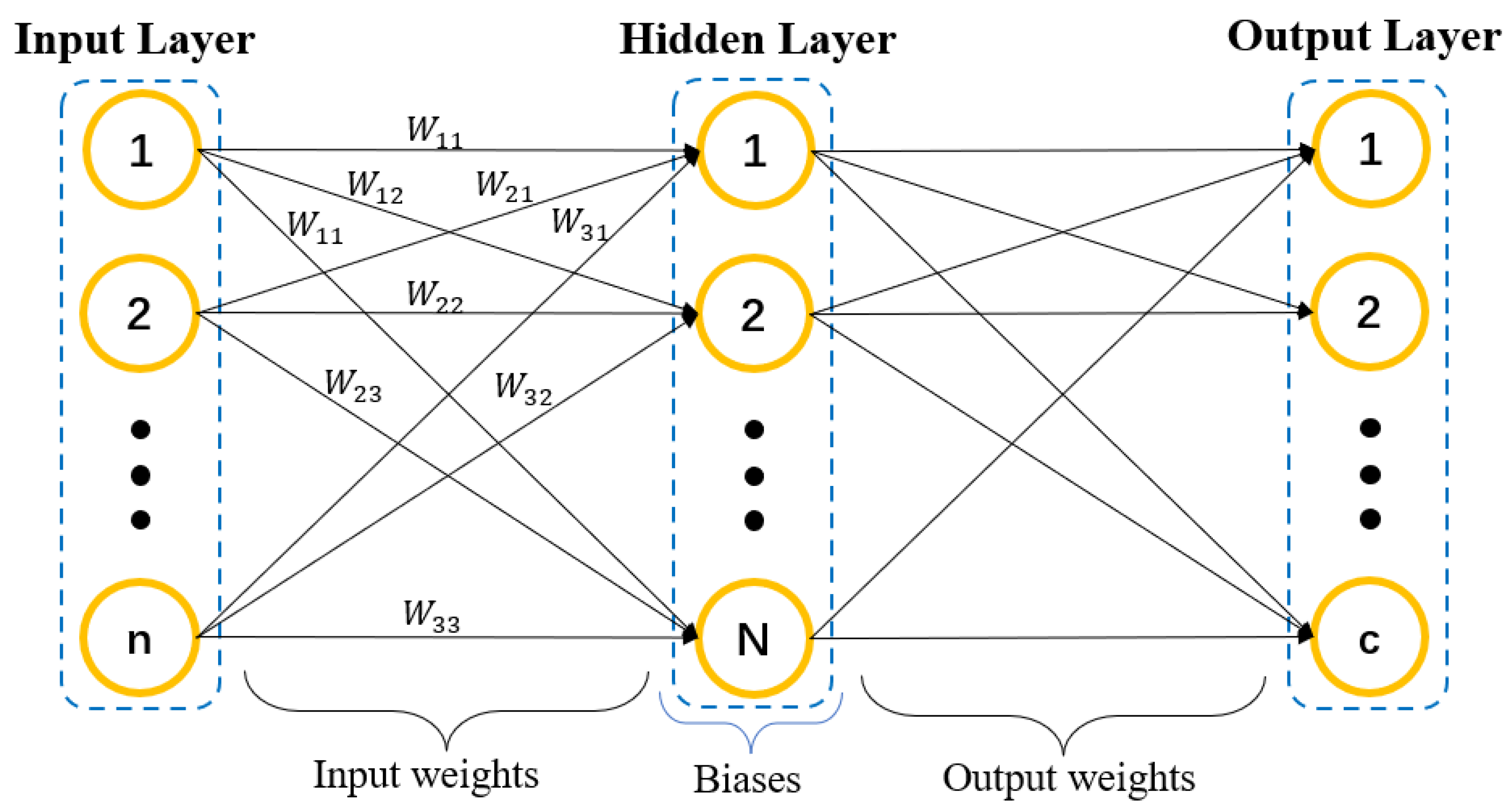
2.1. Original ELM and Kernel ELM

Original ELM stems from single layer feed-forward neural network (SLFN) [10]. In ELM, the input weights w and biases b in hidden layers are stochastically determined.

The output function of ELM can be expressed in Equation (1):

$$f\left(x\right)=\sum _{i=1}^{L}G(w_i,b_i,x)\beta =\sum _{i=1}^L{\beta }_i{h}_i\left(x\right)=h\left(x\right)\beta$$

(1)

where $h\left(x\right)$ is the activation function in the hidden layer, and $h\left(x\right)=[h_1\left(x\right),\dots ,h_L\left(x\right)]$ is the row output vector of hidden layer. $\beta ={[{\beta }_1,\dots ,{\beta }_L]}^T$ is the column vector of the output weights between nodes in the hidden layer and output layer. L is the output dimension. These output weights are generated by linear calculation.

In order to minimize the training error, the training purpose of ELM is illustrated in Equation (2):

$$Minimize:{∥H\beta -T∥}^{2}and∥\beta ∥$$

(2)

where H is the output matrix of hidden layer as shown in Equation (3), and T is the output label matrix:

$$H=\left[\begin{array}{c}h\left(x_1\right)\\ ⋮\\ h\left(x_n\right)\end{array}\right]=\left[\begin{array}{ccc}{h}_1\left(x_1\right)& \cdots & h_L\left(x_1\right)\\ & ⋮& \\ h_1\left(x_n\right)& \cdots & h_L\left(x_n\right)\end{array}\right]$$

(3)

Supposing the training error ${∥H\beta -T∥}^2=0$, then the training work of this model is to find the least-squares solution of a linear system: $H\beta =T$, as Equation (4):

$$\beta =H^{+}T$$

(4)

where $H^{+}$ is the Moore–Penrose pseudo-inverse of H.

According to the Constrained-Optimization theorem, Equation (4) can be improved into Equation (5) (when the number of input samples is not huge):

$$\beta =H^T{(I/C+H{H}^T)}^{-1}T$$

(5)

where I is n-order unit matrix and C is regular cost parameter.

In ref. [17], Huang et al. demonstrated the fundamentals of ELM and proved that ELM can approximate most of the continuous function. Researchers proposed several modified models such as ensemble ELM (E-ELM) [18], bi-directional ELM (B-ELM) [19], and Meta-ELM [20]. Among these methods, kernel ELM (K-ELM) has enhanced the performance of ELM remarkably [21]. In recent years, many researchers have combined ELM models with deep learning [22], transfer learning [23], and random forests [24].

K-ELM [21] defines kernel matrix for ELM, as Equation (6):

$${\Omega }_{ELM}=H{H}^T:{\Omega }_{ELMi,j}=h\left(x_i\right)h\left(x_j\right)=K(x_i,x_j)$$

(6)

It should be mentioned, in K-ELM [21], if kernel function is determined, the vectors of input samples will be transferred from feature space to kernel space.

2.2. ELM-RBF

Unlike ELM, ELM-RBF adopts RBF kernel instead of the single layer feed-forward neural network to improve model’s performance [11]. The centers of clusters and impact widths of RBF kernel are initialized randomly. In addition, the output of the hidden layer is related to the specific task. For instance, in multi-label classification, the dimension of output is equal to the number of categories. In addition, the kernel function in ELM-RBF can be written as Equation (7).

$$h_k\left(x\right)=h(c_k,{\sigma }_k,x)=exp(-{∥x-c_k∥}^2/({\sigma }_k^2)),k=1,2,\dots ,K$$

(7)

where x is the input vector. $c_k$ is the center of the kth cluster in RBF kernel, and ${\sigma }_k$ is the impact width of this cluster.

The result of ELM-RBF is shown as Equation (8).

$$f\left(x\right)=\sum _{i=1}^L{\beta }_i{h}_i\left(x\right)=h\left(x\right)\beta$$

(8)

where ${\beta }_i$ is the output weight.

The optimization target of ELM-RBF can be described as follows:

$$H\beta =T$$

(9)

where H is the output matrix of hidden layer as shown in Equation (3), and T is the output label matrix.

We should mention that RBF function plays a significant role in the original ELM algorithm and its modified models. RBF function is one of the most common activation functions of ELM, and it is also the main kernel style of K-ELM [21]. The selection of activation function for ELM, or the design method for kernel in K-ELM [21], is critical to the performance of model. It is reasonable to believe that the modified ELM model using RBF function as the main structure, such as ELM-RBF, would be an effective algorithm [19].

2.3. Genetic Algorithm

Genetic algorithm is proposed by professor Holland [15] based on the natural selection law of survival of the fittest. Through simulating the biological evolution process and genetic mechanism, GA is more extensible than most traditional optimization methods [25], such as gradient and hill climbing, so it has been used for many complicated engineering problems widely, including neural network, machine learning, function optimization, and so on [26].

GA mainly consists of three operations: selection, crossover, and mutation [27]. The purposes of crossover and mutation are to reconstitute genetic materials of parents and produce unexpected genes to form new individuals. After the above operations, these individuals with higher fitness value will be selected with a relative higher probability to compose a new generation. In general, along with the advance of evolution, the quality of population will be improved gradually [28].

In GAs, the probabilities of crossover ($P_c$) and mutation ($P_m$) determine the performance of algorithm [29] to a large extent. However, the $P_c$ and $P_m$ of simple genetic algorithm (SGA) is constant; as a result, SGA tends to fall into local optimal solution and is difficult to converge in practical application [30].

To address the defect of SGA, some great efforts have been made by many researchers, and the adaptive genetic algorithm (AGA) [31] presented by Srinvas is one of the most representative achievements. Instead of adopting the fixed $P_c$ and $P_m$, in AGA, the $P_c$ and $P_m$ of individuals are adjusted according to respective fitness values, and the result is that the evolutionary quality has been improved greatly [32].

In AGA, these individuals with higher fitness value than the average fitness will vary with lower $P_c$ and $P_m$, and the $P_c$ and $P_m$ of the best individual will be zero [33]. However, in an early evolutionary stage, the local optimum is not necessarily the global optimal solution. Together with the selection mechanism, the population diversity may drop sharply [34]. In addition, the fitness value of individuals including the best will gather near the average fitness, which means their genetic structures are likely to remain unchanged. As a result, the search for the best solution will be handicapped badly, so AGA also has the drawback of premature convergence [35].

Through research and analysis, we present a novel approach to calculate $P_c$ and $P_m$, which makes it possible for the local optimal individuals to amend their genes. In addition, we adopt an adaptive adjustment measure to maintain population diversity, which plays a vital role on preventing premature convergence.

3. Methodology

Because the setting of ELM-RBF is initialized randomly, this kind of model is always unstable and can easily fall into a local optimal solution [14]. To deal with these issues, we propose a modified extreme learning approach, ELM-RBF-SAGA. Specifically, we present a novel genetic algorithm, SAGA, based on two optimization methods firstly. After that, SAGA is used to adjust ILW and HLB to improve model’s prediction accuracy.

3.1. Synergistic Adaptive Genetic Algorithm

In order to improve the optimization performance of SAGA, we present two adaptive optimization measures. One is used for adjusting the range of fitness value to maintain population diversity and provide a solid foundation for evolution. The other is mainly applied to adjust $P_c$ and $P_m$, which are the two crucial factors in suppressing local optimal solutions.

3.1.1. Maintaining the Population Diversity

Along with the advance of evolution, population diversity may stand a good chance of dropping significantly, which means the evolutionary power would be reduced greatly. Especially when dealing some complicated multimodal functions, traditional AGA often falls into local optimum [32,34]. To avoid the above situation as much as possible, we adopt an adjustment measure based on a normal distribution function to prevent the sharp decline of population diversity, and put forward the concept about the expected range of fitness value, denoted by S, whose fundamental purpose is to maintain population diversity by regulating the range of fitness value. The expected range of fitness value in the ith generation $S_i$ can be computed as:

$$\begin{array}{cc}\hfill & S_i=\left\{\begin{array}{cc}{S}_0.exp[\frac{{(c_1.\frac{i}{k})}^2}{-2}],\hfill & R_i⩽S_0.exp[\frac{{(c_1.\frac{i}{k})}^2}{-2}]\hfill \\ R_i,\hfill & R_i⩾S_0.exp[\frac{{(c_1.\frac{i}{k})}^2}{-2}].\hfill \end{array}\right.\hfill \\ \hfill & S_0=R_0\hfill \end{array}$$

(10)

where $R_i$ is the range of fitness in the ith generation. $R_0$ is the range of initial population, and $S_0$ is the expected range of initial population. $c_1$ is a controlled parameter, which equals $\sqrt{2}$ in general. i = 1, 2, 3, …, k, and k is the max number of generations.

As the premise of maintaining population diversity, the expected range of fitness value S is mainly used for setting the maximum difference of fitness value during the adjustment process. In other words, maintaining population diversity should be reflected in the adjustment to individual fitness value finally. Moreover, the relative pecking order of fitness should be invariant, and the absolute difference can be adjusted according to the same ratio. Lastly, as the reference point for adjustment, the average fitness value should be fixed to ensure the stability of evolution. The detailed measures are defined as:

$$f_n^{{}^{\prime }}=\left\{\begin{array}{cc}\overline{f}+(f_n-\overline{f}).\frac{S_i}{R_i},\hfill & \overline{f}+(f_n-\overline{f}).\frac{S_i}{R_i}⩾0\hfill \\ 0,\hfill & \overline{f}+(f_n-\overline{f}).\frac{S_i}{R_i}⩽0\hfill \end{array}\right.$$

(11)

where $f_n$ and $f_n^{{}^{\prime }}$ are the fitness value of the nth individual before and after adjustment, respectively, and $\overline{f}$ is the average fitness value. $R_i$ is the range of fitness in the ith generation, and $S_i$ is the expected range of fitness value in the ith generation.

As shown in Figure 2, the values of a set of samples are 1, 2, 3, and 4, denoted by a, b, c, and d, and b is the average value. Obviously, the range R equals d-a, namely 3. If S is set to 7, according to the measures above, the values of these samples would be revised as −0.333, 2, 4.333, and 6.666, denoted by $a_1$, $b_1$, $c_1$, $d_1$. The following are the detailed analyses. Firstly, $b_1$ equals to b, in other words, the average value is unchanged. Secondly, the max difference is $d_1-a_1$, namely 6.999, which is very close to S. In addition, the relative positions of these samples are invariant, for instance, $b-a$ = $c-b$, $d-b$ = 2($c-b$) and $b_1-a_1$ = $c_1-b_1$, $d_1-b_1$ = 2($c_1-b_1$) correspondingly. Based on these analyses, the purpose of adjustment has been achieved perfectly.

3.1.2. Adaptive Probabilities of Crossover and Mutation

In GAs, $P_c$ and $P_m$ play a vital role in preventing premature convergence [33]. In AGA, the $P_c$ and $P_m$ of the best individuals are both zero, which means they will be preserved into the next generation [34]. However, they may not be the global optimal individuals. With the advance of evolution, the algorithm will get stuck at a local optimum easily [32]. To overcome the weakness of AGA, we adopt a new method based on normal distribution to calculate $P_c$ and $P_m$, and the method can be expressed as:

$$P_m=\left\{\begin{array}{cc}{P}_{Mmin}+(P_{Mmax}-P_{Mmin}).exp[\frac{{(c_2.\frac{f-\overline{f}}{f_{max}-\overline{f}})}^2}{-2}],\hfill & f⩾\overline{f}\hfill \\ P_{Mmax},\hfill & f⩽\overline{f}\hfill \end{array}\right.$$

(12)

$$P_c=\left\{\begin{array}{cc}{P}_{Cmin}+(P_{Cmax}-P_{Cmin}).exp[\frac{{(c_3.\frac{f^{{}^{\prime }}-\overline{f}}{f_{max}-\overline{f}})}^2}{-2}],\hfill & f⩾\overline{f}\hfill \\ P_{Cmax},\hfill & f⩽\overline{f}\hfill \end{array}\right.$$

(13)

where $P_{Mmax}$, $P_{Mmin}$, $P_{Cmax}$ and $P_{Cmin}$ are the maximum and minimum value of $P_c$ and $P_m$, respectively. $f_{max}$ is the maximum fitness value of population. $\overline{f}$ is denoted as the average fitness value, and $f^{{}^{\prime }}$ is the larger fitness value of the individuals to be crossed. $c_2$ and $c_3$ are the controlled parameters, and both equal to 3 in general.

The adaptive adjustment curves of $P_c$ and $P_m$ are shown in Figure 3 and Figure 4.

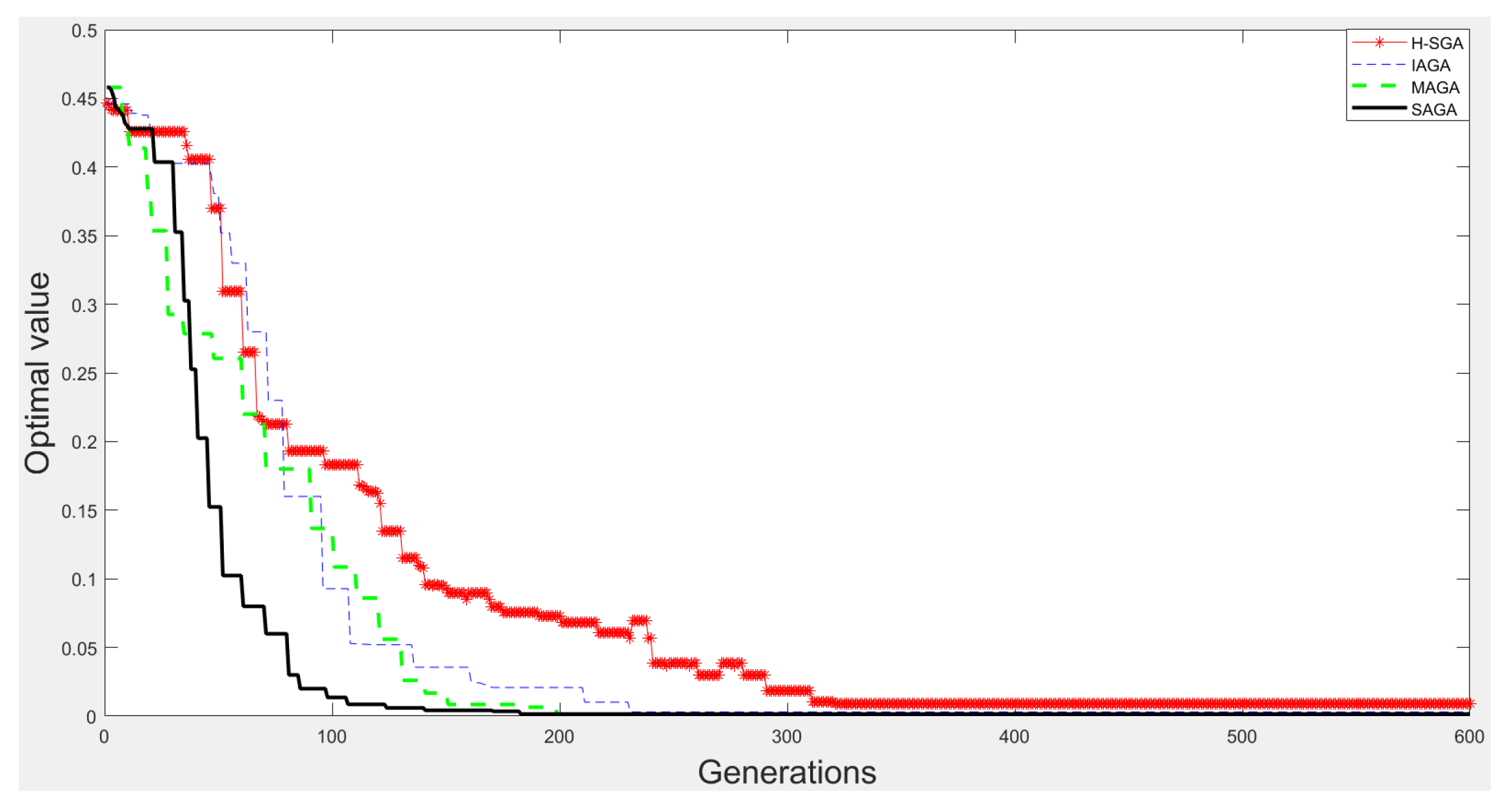
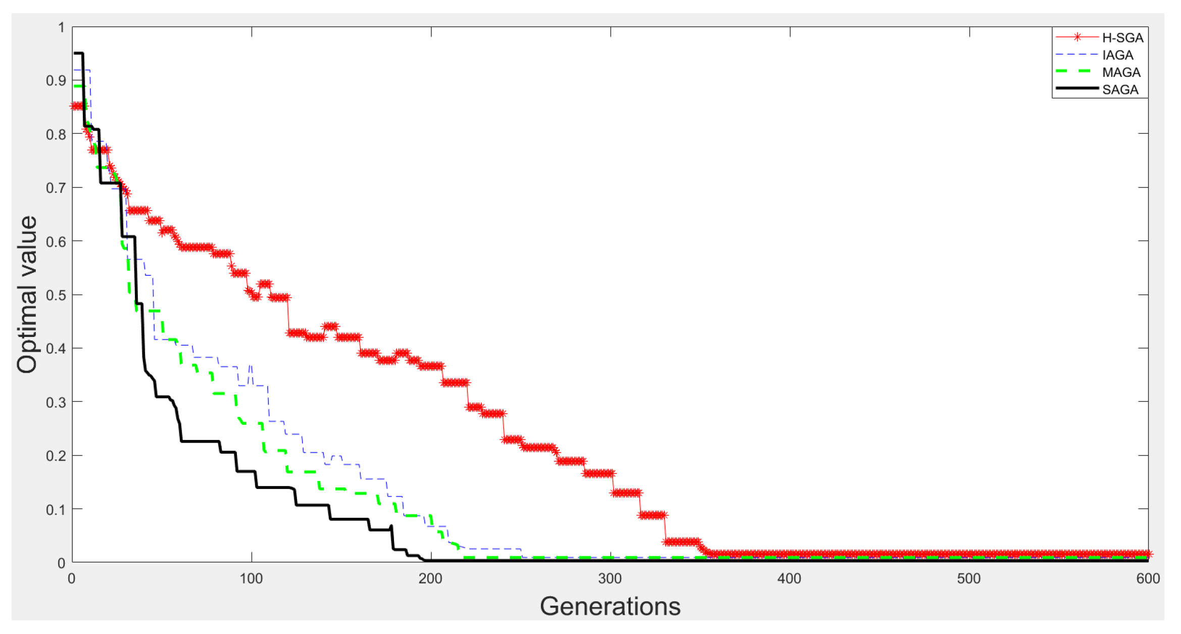
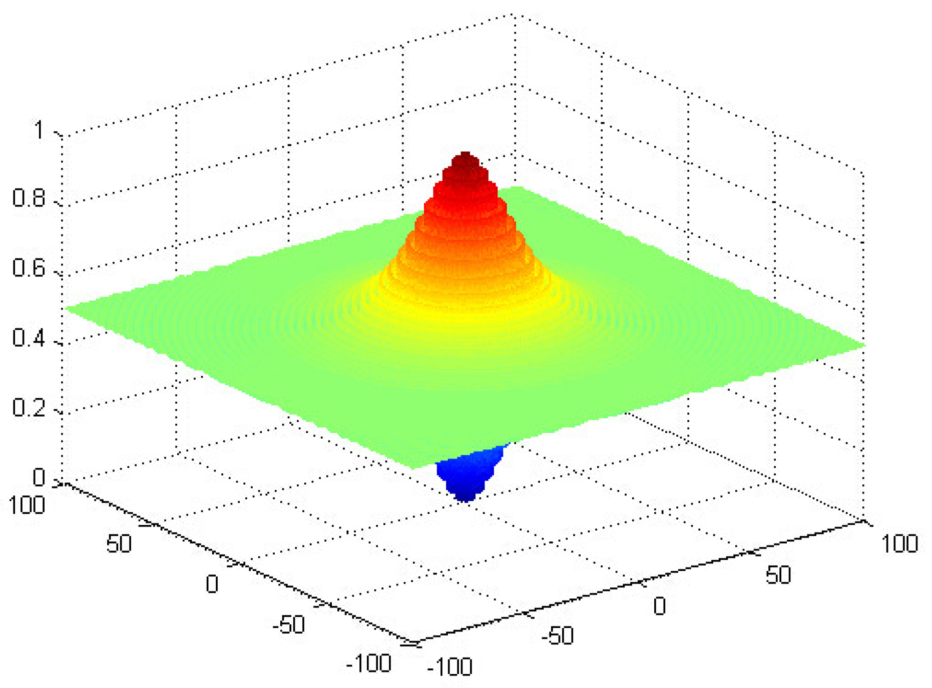
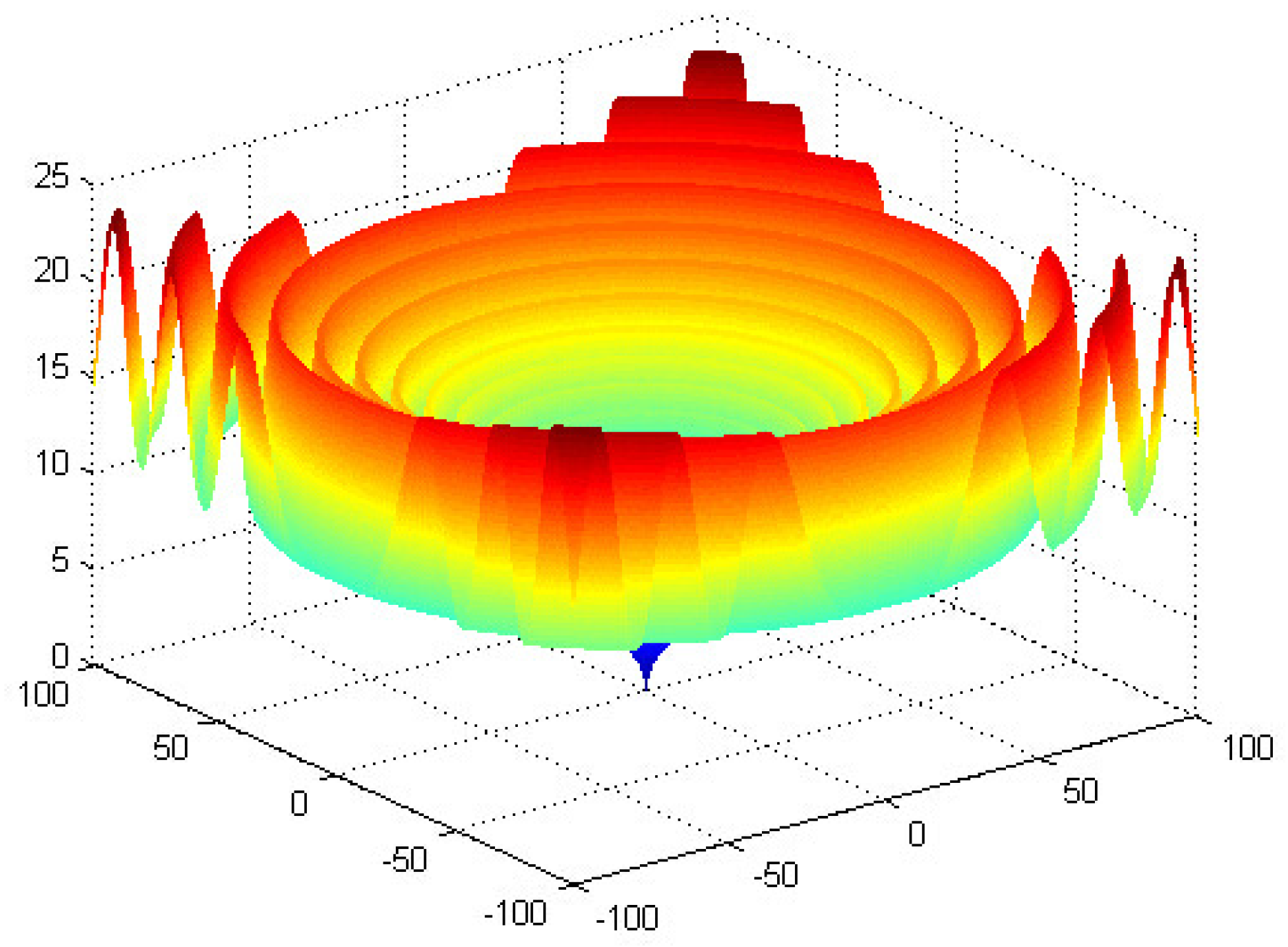
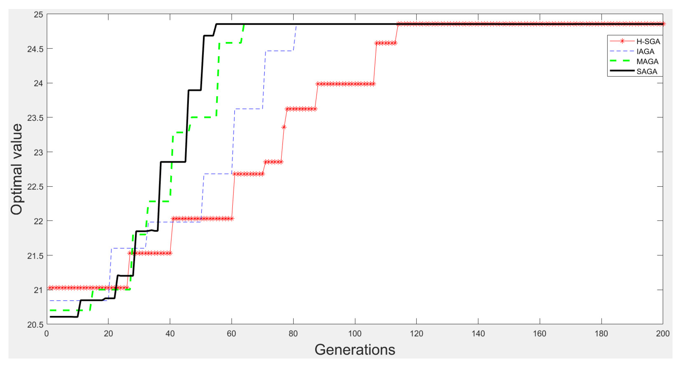
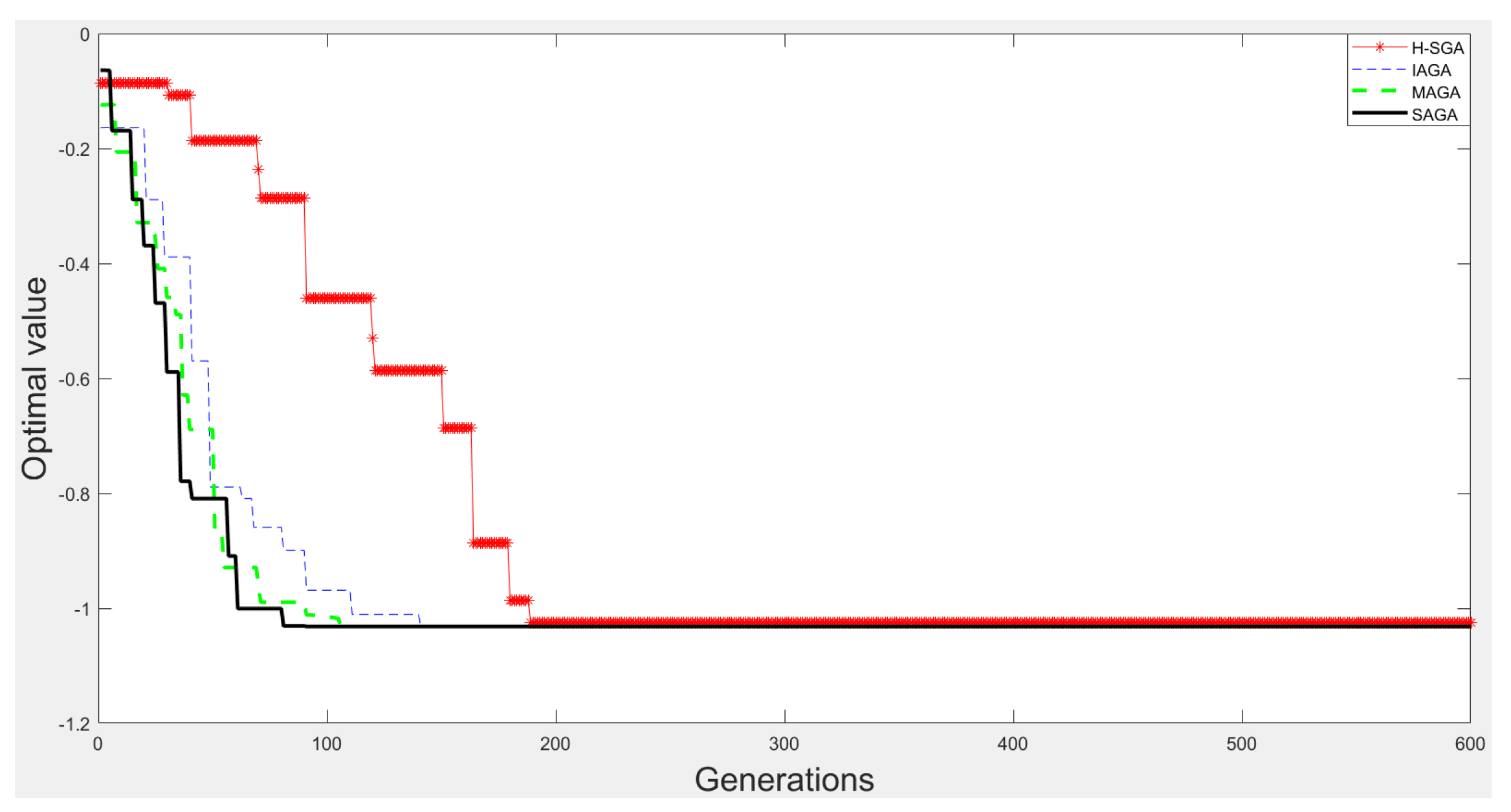
3.1.3. Optimization Experiments

In order to test the optimization performance of SAGA, compared with H-SGA [36], IAGA [37], and MAGA [38], we select several classical functions to carry out the comparing experiments. These functions are shown as below:

$F_1$: One-dimension multimodal function.

$$\begin{gathered} F_1=x+10sin(5x)+7cos(4x), \\ 0⩽x⩽9 \end{gathered}$$

(14)

This function has multiple local optima in x∈$\left[0,9\right]$, and the only one maximum is $F_1$ (7.8568) = 24.8554. The graph of $F_1$ is shown in Figure 5.

$F_2$: Camel function.

$$\begin{gathered} F_2=(4-2.1x_1^2+\frac{x_1^2}{3})x_1^2+x_1{x}_2+(-4+x_2^2)x_2^2, \\ -3⩽x_i⩽3,i=1,2 \end{gathered}$$

(15)

This function has six local minima and two global minima, which are $F_2$(−0.0898, 0.7126) = $F_2$(0.0898, −0.7126) = −1.031628. The graph of $F_2$ is shown in Figure 6.

$F_3$: Schaffer’s $f_6$ [39].

$$\begin{gathered} F_3=0.5+\frac{{sin}^2\sqrt{x_1^2+x_2^2}-0.5}{{[1.0+0.001(x_1^2+x_2^2)]}^2}, \\ -100⩽x_i⩽100,i=1,2 \end{gathered}$$

(16)

The function is symmetric about the origin and has multiple local optimal values. Its global minimum is $F_3$(0, 0) = 0. As a result, this function is very suitable for optimization experiment. The graph of $F_3$ is shown in Figure 7.

$F_4$: Schaffer’s $f_7$ [39].

$$\begin{gathered} F_4={(x_1^2+x_2^2)}^{0.25}[{sin}^2(50{(x_1^2+x_2^2)}^{0.1})+0.1], \\ -100⩽x_i⩽100,i=1,2 \end{gathered}$$

(17)

This function is similar to $F_3$, and its global minimum is $F_4$(0, 0) = 0. The graph of $F_4$ is shown in Figure 8.

In all experiments, the size of population is 20, and the binary length is 22. The number of iterations in $F_1$ is 200, and that of in other function is 600. In H-SGA [36], $P_c$ is altering from 0.5 to 0.75, and $P_m$ is altering from 0.05 to 0.08. The range of $P_c$ in IAGA [37] and SAGA is (0.6, 0.8), and that of $P_m$ is (0.05, 0.08). In MAGA [38], $P_{c1}$ = 0.7, $P_{c2}$ = 0.2, $P_{m1}$ = 0.07, $P_{m2}$ = 0.03, $\gamma$ = 2 and $\alpha$ = 0.08.

Based on the above conditions, each function is executed 1000 times independently with four algorithms in an initial environment randomly. In addition, the calculation accuracy of function $F_1$ and $F_2$ is ${10}^{-4}$, and that of $F_3$ and $F_4$ is ${10}^{-6}$.

Table 1. The total number of convergences.

Method	Multimodal Function
	${\mathit{F}}_{\mathbf{1}}$	${\mathit{F}}_{\mathbf{2}}$	${\mathit{F}}_{\mathbf{3}}$	${\mathit{F}}_{\mathbf{4}}$
H-SGA [36]	980	964	753	625
IAGA [37]	993	982	895	863
MAGA [38]	996	991	966	953
SAGA	1000	997	995	986

,

Table 2. Average convergence generation.

Method	Multimodal Function
	${\mathit{F}}_{\mathbf{1}}$	${\mathit{F}}_{\mathbf{2}}$	${\mathit{F}}_{\mathbf{3}}$	${\mathit{F}}_{\mathbf{4}}$
H-SGA [36]	113	191	320	356
IAGA [37]	82	133	263	272
MAGA [38]	62	105	198	215
SAGA	56	95	183	196

and

Table 3. Average convergence value.

Method	Multimodal Function
	${\mathit{F}}_{\mathbf{1}}$	${\mathit{F}}_{\mathbf{2}}$	${\mathit{F}}_{\mathbf{3}}$	${\mathit{F}}_{\mathbf{4}}$
H-SGA [36]	24.825632	−1.028323	0.0094	0.0150
IAGA [37]	24.850056	−1.031200	0.0030	0.0092
MAGA [38]	24.853056	−1.031300	0.0022	0.0042
SAGA	24.855368	−1.031601	0.0016	0.0035

list the experimental results, for example, the number of convergences, average convergence generation, and value.

From Table 1 and Table 2, we can easily find that SAGA and MAGA [38] have higher convergence rates and fewer iterations compared with H-SGA [36] and IAGA [37], which indicates these two methods have obvious advantages in convergence speed. However, as shown in Table 3, SAGA is better than MAGA [38] in the final convergence result, which fully proves the method proposed in this paper has outstanding global optimization ability. Figure 9, Figure 10, Figure 11 and Figure 12 are the experimental results of the comparison algorithm on each optimization function.

From Figure 9, Figure 10, Figure 11 and Figure 12, we can clearly find that SAGA and MAGA [38] outperform H-SGA [36] and IAGA [37] in terms of convergent speed and robustness. In addition, the performance of SAGA is close to that of MAGA [38] on the experiments with function $F_1$ and $F_2$. Benefitting from the adjustment method of maintaining population diversity, SAGA can obtain the global optimal solutions easily on the experiments about $F_3$ and $F_4$, which is superior to MAGA [38]. In summary, SAGA has the excellent ability to search global optimal solutions and can converge quickly.

3.2. ELM-RBF-SAGA

Due to the lack of effective optimization for ILW and HLB, conventional ELM-RBF is often unstable and prone to falling into local optimal solutions [14]. Considering SAGA’s extraordinary optimization ability as shown in Section 3.1.3, we introduce SAGA into ELM-RBF to adjust ILW and HLB for improving model’s prediction accuracy. Specifically, ILW and HLB are firstly mapped to individual vectors in SAGA. Then, the overall error function of training set and test set is taken as SAGA’s fitness function, which can be described by Equation (18). In addition, the prediction error of ELM-RBF-SAGA will be gradually reduced through iterative optimization operations, such as crossover, mutation, and selection. As a result, the optimal ILW and HLB are used to minimize error:

$$Fitness\left(S\right)=\sqrt{\frac{1}{n}\sum _{i=1}^n{\left(f\left(x_i\right)-y_i\right)}^2}$$

(18)

where S = {($x_i$, $y_i$)∣ 0 < i⩽n} is the dataset. $x_i$ is the input instance as shown in Equation (7), $y_i$ is the real label corresponding to $x_i$, and n is the number of instances. $f(.)$ is the output of ELM-RBF as shown in Equation (8).

The detailed steps of ELM-RBF-SAGA are described as below.

• Build ELM-RBF network model.
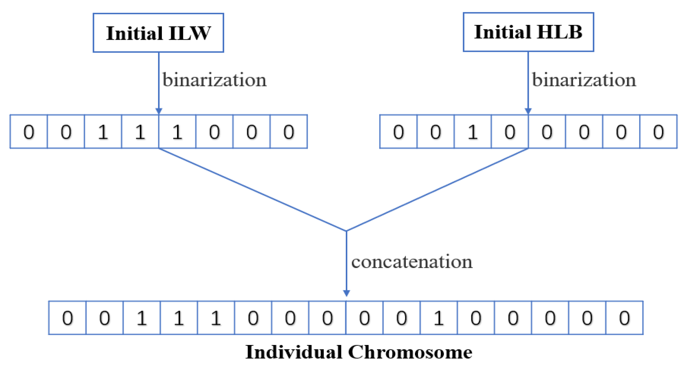
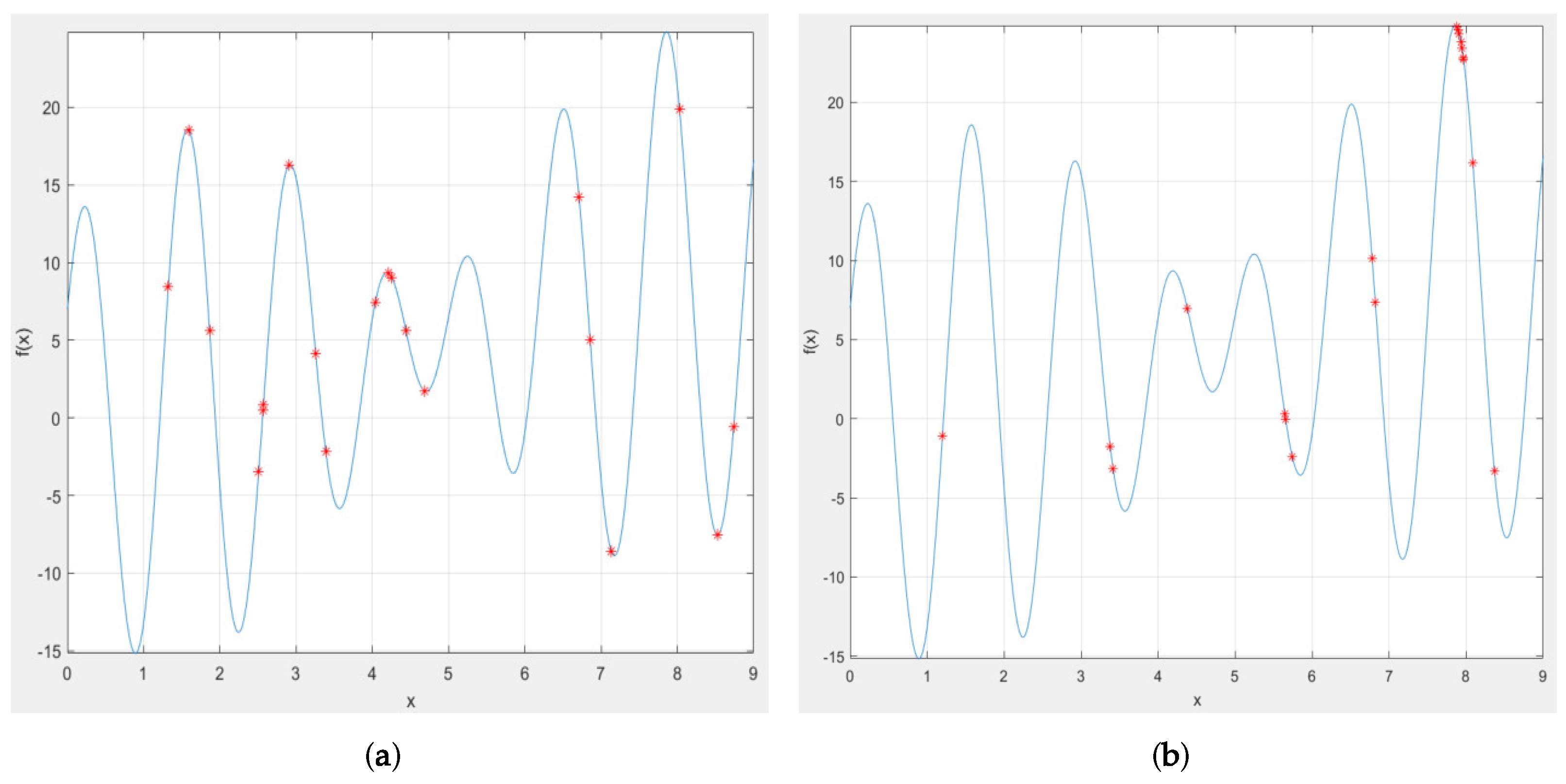
• Initialize population in SAGA. ILW and HLB of ELM-RBF are encoded in individual genes as shown in Figure 13, and the evolutionary population is initialized accordingly. Figure 14 demonstrates the variation trend of population before and after evolution. It can be clearly seen from Figure 14a that the initial individuals are aimlessly distributed. However, after iterative optimization, the population is consciously close to the global optimal position as exhibited in Figure 14b.
• Set fitness function of SAGA. The error function of ELM-RBF is taken as the fitness function of SAGA, and then the fitness values of initial population are calculated.
• Perform selecting operation. With the continuous advancement of evolution, the calculation error will gradually be reduced. As a result, it is necessary to take the reciprocal of fitness function to select the individuals with “high fitness”.
• Adjust individual fitness according to Equations (10) and (11).
• Update the $P_c$ and $P_m$ in SAGA according to Equations (12) and (13).
• Perform crossover and mutation according to new $P_c$ and $P_m$.
• Compute the fitness value of new individual based on Equation (18). These individuals with superior performance are preserved to compose the next evolutionary group.
• Iterate steps 4–8 until the termination condition is satisfied, for instance, the number of iterations or the minimum error.
• Decode the individual gene with the best fitness value. ELM-RBF is initialized with the decoded ILW and HLB to obtain the optimal network structure, which is used for multi-label classification as shown in Section 2.2.

4. Experiments and Discussion

4.1. Comparing Algorithms

We choose four remarkable methods to perform comparative experiments with ELM-RBF-SAGA about multi-label classification. These algorithms are described as follows:

• ML-KNN [40]: This model is a classic multi-label classification approach.
• ML-ELM-RBF [41]: This model extends ELM-RBF to deal with multi-label classification.
• ML-KELM [42]: This model makes use of an efficient projection framework to produce an optimal solution.
• ML-CK-ELM [43]: In this model, a specific module is constructed based on several predefined kernels to promote classification accuracy.

4.2. Experimental Datasets

Following the classical method in [40], we choose four general datasets, which are widely applied to assess the model’s ability in multi-label classification, to perform the validation experiment. They are “Art dataset”, “Business dataset”, “Computer dataset”, and “Yeast dataset”.

Table 4. Details about the multi-label classification datasets.

Dataset	Train	Test	Dim	Label
Art  [40]	2000	3000	462	26
Business [40]	2000	3000	438	30
Computer [40]	2000	3000	681	33
Yeast [40]	1500	917	103	14

lists the details of these datasets.

4.3. Evaluation Metrics

In this paper, we select some universal evaluation metrics, such as Hamming loss, one-error, coverage, ranking loss, and average precision, to verify the classification effect of different models. These metrics are shown as the following formulas. In these formulas, S = {($x_i$, $y_i$)∣ 0 < i⩽n} is the dataset, $h(.)$ is the multi-label classification model, n is the number of input instances, and q is the output dimension and the number of labels for each instance. $x_i$ is the set of input samples, $y_i$ is the set of output values. $Y_i$ is the set of labels, l is the subset of $Y_i$. $f(.)$ is the objective function. $ran{k}_f(.)$ is the ranking function.

Hamming loss indicates the gap between outputs of classifier and the true label and can be defined as:

$$HammingLos{s}_S\left(h\right)=\frac{1}{n}\sum _{i=1}^n\frac{1}{q}\left|h\left(x_i\right)\Delta Y_i\right|$$

(19)

where $h\left(x_i\right)$$\Delta$$Y_i$ means the symmetric difference between outputs and ground-truth.

One-error is used for evaluating the times that top-ranked label is not in the set of relevant labels. In addition, the computational process is expressed as:

$${One-Error}_S\left(h\right)=\frac{1}{n}\sum _{i=1}^n\frac{1}{q}[[arg\underset{p\in y_i}{max}f(x_i,p)]\notin Y_i]$$

(20)

Coverage, as shown in Equation (21), reveals the minimum query times of finding all the relevant labels in a sequence of output set:

$${Coverage}_S\left(h\right)=\frac{1}{n}\sum _{i=1}^n\underset{l\in Y_i}{max}ran{k}_f(x_i,l)-1$$

(21)

Ranking loss measures the average fraction that the irrelevant labels are in front of the relevant labels in a rank of output values associated with an input instance. The computational process is described as follows:

$${RankingLoss}_S\left(h\right)=\frac{1}{n}\sum _{i=1}^n\frac{1}{|Y_i\left|\right|\overline{Y_i}|}\left|\{(l_1,l_2)\mid f(x_i,l_1)⩽f(x_i,l_2),(l_1,l_2)\in Y_i\times \overline{Y_i}\}\right|$$

(22)

where $\overline{Y_i}$ denotes the complementary set of $Y_i$ in the label space Y.

Average precision evaluates the average fraction of relevant labels ranked above a particular label. This indicator can be formulated by the following equation:

$${AveragePrecision}_S\left(h\right)=\frac{1}{n}\sum _{i=1}^n\frac{1}{|Y_i|}\sum _{l\in Y_i}\frac{\left|\right\{l^{{}^{\prime }}\mid ran{k}_f(x_i,l^{{}^{\prime }})⩽ran{k}_f(x_i,l),l^{{}^{\prime }}\in Y_i\left\}\right|}{ran{k}_f(x_i,l)}$$

(23)

4.4. Experimental Results and Discussion

Experimental results in different datasets are shown in

Table 5. Performance of different models in the art dataset.

Evaluation Metric	Algorithm
	ML-KNN [40]	ML-ELM-RBF [41]	ML-KELM [42]	ML-CK-ELM [43]	ELM-RBF-SAGA
Average Precision	0.5736	0.6078	0.6132	0.6263	0.6317
Coverage	4.7539	5.6723	5.2531	4.5864	4.5826
Hamming Loss	0.0576	0.0535	0.0531	0.0553	0.0533
One-Error	0.5132	0.4739	0.4732	0.4698	0.4683
Ranking Loss	0.1273	0.1387	0.1126	0.1143	0.1131

,

Table 6. Performance of different models in the yeast dataset.

Evaluation Metric	Algorithm
	ML-KNN [40]	ML-ELM-RBF [41]	ML-KELM [42]	ML-CK-ELM [43]	ELM-RBF-SAGA
Average Precision	0.7541	0.7567	0.7623	0.7778	0.7773
Coverage	6.3986	6.4632	6.2573	6.1935	6.1893
Hamming Loss	0.1953	0.1968	0.1858	0.1864	0.1845
One-Error	0.2345	0.2376	0.2292	0.2268	0.2285
Ranking Loss	0.1719	0.1728	0.1613	0.1593	0.1586

,

Table 7. Performance of different models in the business dataset.

Evaluation Metric	Algorithm
	ML-KNN [40]	ML-ELM-RBF [41]	ML-KELM [42]	ML-CK-ELM [43]	ELM-RBF-SAGA
Average Precision	0.8826	0.8835	0.8863	0.8872	0.8886
Coverage	2.1576	2.5076	2.4964	2.4058	2.4032
Hamming Loss	0.0261	0.0258	0.0256	0.0232	0.0241
One-Error	0.1213	0.1163	0.1143	0.1156	0.1135
Ranking Loss	0.0356	0.0392	0.0369	0.0376	0.0342

and

Table 8. Performance of different models in the computer dataset.

Evaluation Metric	Algorithm
	ML-KNN [40]	ML-ELM-RBF [41]	ML-KELM [42]	ML-CK-ELM [43]	ELM-RBF-SAGA
Average Precision	0.6718	0.6983	0.7021	0.7112	0.7136
Coverage	3.9417	4.3896	3.9863	3.9578	3.9286
Hamming Loss	0.0362	0.0332	0.0339	0.0341	0.0336
One-Error	0.3960	0.3329	0.3526	0.3418	0.3345
Ranking Loss	0.0787	0.0913	0.0856	0.0793	0.0785

, respectively. As a classical multi-label classification method, ML-KNN [40] distinguishes categories by measuring the distance between different feature values. This method is simple and insensitive to abnormal input. However, compared with ELM-based methods, the performance of ML-KNN [40] is always unsatisfactory, which also indicates the effectiveness of ELM. ML-ELM-RBF [41] improves the classification accuracy of ELM-RBF by stacking ELM-AE. Compared with ML-KNN [40], the performance of ML-ELM-RBF [41] is significantly improved, such as acquiring the best values of Hamming loss and one-error in computer dataset. To search the optimal solution, ML-KELM [42] employs a special projection framework and non-singular transformation matrix. Experimental results show that this method achieves competitive performance, especially obtaining the optimal values of Hamming loss and ranking loss in the art dataset. ML-CK-ELM [43] improves multi-label classification accuracy by optimizing the combination of multiple kernels; as a result, this approach is better than these previous methods in most indicators. Although without multi-layer staked structure, ELM-RBF-SAGA proposed in this paper is superior to ML-CK-ELM [43] on the whole, which fully demonstrates the effectiveness of SAGA in optimizing ELM-RBF.

Table 9. Running time of different models in each dataset.

Evaluation Metric	Algorithm
	ML-KNN [40]	ML-ELM-RBF [41]	ML-KELM [42]	ML-CK-ELM [43]	ELM-RBF-SAGA
Training time in Art [40]	1.2365	1.1735	1.1967	1.2132	1.2053
Testing time in Art [40]	1.1986	1.1552	1.1624	1.1862	1.1775
Training time in Business [40]	2.4573	1.8521	1.9173	2.0681	2.1367
Testing time in Business [40]	2.1061	1.7647	1.8265	1.8572	1.9356
Training time in Computer [40]	2.8732	2.1369	2.2358	2.3537	2.2132
Testing time in Computer [40]	2.6113	1.9127	2.0526	2.1769	2.0319
Training time in Yeast [40]	1.0523	0.7631	0.8256	0.9572	0.8543
Testing time in Yeast [40]	0.8958	0.7239	0.7653	0.8839	0.7668

lists the running time of different models in each dataset. It can be easily found from Table 9, as the representative of traditional machine learning methods, ML-KNN [40] is significantly slower than ELM-based models whether in the training or testing phase. In addition, this trend is especially evident with dataset’s complexity increasing. Although our proposed method is not the fastest, it is faster than ML-CK-ELM [43] in art, computer, and yeast dataset. In summary, ELM-RBF-SAGA has obvious advantages over comparison methods and is very suitable for multi-label classification.

5. Conclusions

Because of the lack of effective optimization methods, conventional ELM-RBF is always unstable has difficulty finding the global optimal solution, which leads to inferior prediction precision in multi-label classification. Aiming at these issues, a modified extreme learning model, ELM-RBF-SAGA, is proposed in this article.. In ELM-RBF-SAGA, an improved genetic algorithm, SAGA, is presented to optimize the performance of ELM-RBF. In addition, two adjustment methods are employed cooperatively in SAGA. One is applied to adjust the range of fitness value for maintaining population diversity, the other is used for updating crossover and mutation probability to generate the optimal ILW and HLB in ELM-RBF. Experiments suggest that our proposed method achieves overwhelming advantages in multi-label classification.

References

1. Read, J.; Pfahringer, B.; Holmes, G.; Frank, E. Classifier chains for multi-label classification. Mach. Learn. 2011, 85, 333–359. [Google Scholar] [CrossRef] [Green Version]
2. Zhang, M.; Zhou, Z. A Review on Multi-Label Learning Algorithms. IEEE Trans. Knowl. Data Eng. 2014, 26, 1819–1837. [Google Scholar] [CrossRef]
3. Hüllermeier, E.; Fürnkranz, J.; Cheng, W.; Brinker, K. Label ranking by learning pairwise preferences. Artif. Intell. 2008, 172, 1897–1916. [Google Scholar] [CrossRef] [Green Version]
4. Huang, G.; Zhou, H.; Ding, X.; Zhang, R. Extreme Learning Machine for Regression and Multiclass Classification. IEEE Trans. Syst. Man Cybern. Part B 2012, 42, 513–529. [Google Scholar] [CrossRef] [Green Version]
5. Huang, G.; Zhu, Q.; Siew, C.K. Extreme learning machine: Theory and applications. Neurocomputing 2006, 70, 489–501. [Google Scholar] [CrossRef]
6. Li, J.; Shi, X.; You, Z.; Yi, H.; Chen, Z.; Lin, Q.; Fang, M. Using Weighted Extreme Learning Machine Combined With Scale-Invariant Feature Transform to Predict Protein-Protein Interactions From Protein Evolutionary Information. IEEE ACM Trans. Comput. Biol. Bioinform. 2020, 17, 1546–1554. [Google Scholar] [CrossRef]
7. Liang, X.; Zhang, H.; Lu, T.; Gulliver, T.A. Extreme learning machine for 60 GHz millimetre wave positioning. IET Commun. 2017, 11, 483–489. [Google Scholar] [CrossRef]
8. Cervellera, C.; Macciò, D. An Extreme Learning Machine Approach to Density Estimation Problems. IEEE Trans. Cybern. 2017, 47, 3254–3265. [Google Scholar] [CrossRef]
9. Liang, Q.; Wu, W.; Coppola, G.; Zhang, D.; Sun, W.; Ge, Y.; Wang, Y. Calibration and decoupling of multi-axis robotic Force/Moment sensors. Robot.-Comput.-Integr. Manuf. 2018, 49, 301–308. [Google Scholar] [CrossRef]
10. Chen, H.; Gao, P.; Tan, S.; Tang, J.; Yuan, H. Online sequential condition prediction method of natural circulation systems based on EOS-ELM and phase space reconstruction. Ann. Nucl. Energy 2017, 110, 1107–1120. [Google Scholar] [CrossRef]
11. Huang, G.; Siew, C.K. Extreme learning machine: RBF network case. In Proceedings of the 8th International Conference on Control, Automation, Robotics and Vision, ICARCV 2004, Kunming, China, 6–9 December 2004; pp. 1029–1036. [Google Scholar] [CrossRef]
12. Niu, M.; Zhang, J.; Li, Y.; Wang, C.; Liu, Z.; Ding, H.; Zou, Q.; Ma, Q. CirRNAPL: A web server for the identification of circRNA based on extreme learning machine. Comput. Struct. Biotechnol. J. 2020, 18, 834–842. [Google Scholar] [CrossRef]
13. Wong, P.; Huang, W.; Vong, C.; Yang, Z. Adaptive neural tracking control for automotive engine idle speed regulation using extreme learning machine. Neural Comput. Appl. 2020, 32, 14399–14409. [Google Scholar] [CrossRef]
14. Nilesh, R.; Sunil, W. Improving Extreme Learning Machine through Optimization A Review. In Proceedings of the 7th International Conference on Advanced Computing and Communication Systems (ICACCS), Coimbatore, India, 19–20 March 2021; IEEE: Piscataway, NJ, USA, 2021; pp. 906–912. [Google Scholar] [CrossRef]
15. Holland, J.H. Adaptation in Natural and Artificial Systems: An Introductory Analysis with Applications to Biology, Control, and Artificial Intelligence; MIT Press: Cambridge, MA, USA, 1992. [Google Scholar] [CrossRef]
16. Tahir, M.; Tubaishat, A.; Al-Obeidat, F.; Shah, B.; Halim, Z.; Waqas, M. A novel binary chaotic genetic algorithm for feature selection and its utility in affective computing and healthcare. Neural Comput. Appl. 2020, 1–22. [Google Scholar] [CrossRef]
17. Huang, G. An Insight into Extreme Learning Machines: Random Neurons, Random Features and Kernels. Cogn. Comput. 2014, 6, 376–390. [Google Scholar] [CrossRef]
18. Yang, R.; Xu, S.; Feng, L. An Ensemble Extreme Learning Machine for Data Stream Classification. Algorithms 2018, 11, 107. [Google Scholar] [CrossRef] [Green Version]
19. Rajpal, A.; Mishra, A.; Bala, R. A Novel fuzzy frame selection based watermarking scheme for MPEG-4 videos using Bi-directional extreme learning machine. Appl. Soft Comput. 2019, 74, 603–620. [Google Scholar] [CrossRef]
20. Zou, W.; Yao, F.; Zhang, B.; Guan, Z. Improved Meta-ELM with error feedback incremental ELM as hidden nodes. Neural Comput. Appl. 2018, 30, 3363–3370. [Google Scholar] [CrossRef]
21. Wang, M.; Chen, H.; Li, H.; Cai, Z.; Zhao, X.; Tong, C.; Li, J.; Xu, X. Grey wolf optimization evolving kernel extreme learning machine: Application to bankruptcy prediction. Eng. Appl. Artif. Intell. 2017, 63, 54–68. [Google Scholar] [CrossRef]
22. Ding, S.; Guo, L.; Hou, Y. Extreme learning machine with kernel model based on deep learning. Neural Comput. Appl. 2017, 28, 1975–1984. [Google Scholar] [CrossRef]
23. Salaken, S.M.; Khosravi, A.; Nguyen, T.; Nahavandi, S. Extreme learning machine based transfer learning algorithms: A survey. Neurocomputing 2017, 267, 516–524. [Google Scholar] [CrossRef]
24. Lin, L.; Wang, F.; Xie, X.; Zhong, S. Random forests-based extreme learning machine ensemble for multi-regime time series prediction. Expert Syst. Appl. 2017, 83, 164–176. [Google Scholar] [CrossRef]
25. Peerlinck, A.; Sheppard, J.; Pastorino, J.; Maxwell, B. Optimal Design of Experiments for Precision Agriculture Using a Genetic Algorithm. In Proceedings of the IEEE Congress on Evolutionary Computation, Wellington, New Zealand, 10–13 June 2019; pp. 1838–1845. [Google Scholar] [CrossRef]
26. Liu, D. Mathematical modeling analysis of genetic algorithms under schema theorem. J. Comput. Methods Sci. Eng. 2019, 19, 131–137. [Google Scholar] [CrossRef]
27. Sari, M.; Tuna, C. Prediction of Pathological Subjects Using Genetic Algorithms. Comput. Math. Methods Med. 2018, 2018, 6154025. [Google Scholar] [CrossRef] [PubMed] [Green Version]
28. Pattanaik, J.K.; Basu, M.; Dash, D.P. Improved real coded genetic algorithm for dynamic economic dispatch. J. Electr. Syst. Inf. Technol. 2018, 5, 349–362. [Google Scholar] [CrossRef]
29. Rafsanjani, M.K.; Riyahi, M. A new hybrid genetic algorithm for job shop scheduling problem. Int. J. Adv. Intell. Paradig. 2020, 16, 157–171. [Google Scholar] [CrossRef]
30. Maghawry, A.; Kholief, M.; Omar, Y.M.K.; Hodhod, R. An Approach for Evolving Transformation Sequences Using Hybrid Genetic Algorithms. Int. J. Comput. Intell. Syst. 2020, 13, 223–233. [Google Scholar] [CrossRef] [Green Version]
31. Srinivas, M.; Patnaik, L.M. Adaptive probabilities of crossover and mutation in genetic algorithms. IEEE Trans. Syst. Man Cybern. 1994, 24, 656–667. [Google Scholar] [CrossRef] [Green Version]
32. Wang, J.; Zhang, M.; Ersoy, O.K.; Sun, K.; Bi, Y. An Improved Real-Coded Genetic Algorithm Using the Heuristical Normal Distribution and Direction-Based Crossover. Comput. Intell. Neurosci. 2019, 2019, 4243853. [Google Scholar] [CrossRef]
33. Li, Y.B.; Sang, H.B.; Xiong, X.; Li, Y.R. An improved adaptive genetic algorithm for two-dimensional rectangular packing problem. Appl. Sci. 2021, 11, 413. [Google Scholar] [CrossRef]
34. Xiang, X.; Yu, C.; Xu, H.; Zhu, S.X. Optimization of Heterogeneous Container Loading Problem with Adaptive Genetic Algorithm. Complexity 2018, 2018, 2024184. [Google Scholar] [CrossRef] [Green Version]
35. Zhang, R.; Ong, P.S.; Nee, A.Y.C. A simulation-based genetic algorithm approach for remanufacturing process planning and scheduling. Appl. Soft Comput. 2015, 37, 521–532. [Google Scholar] [CrossRef]
36. Jiang, J.; Yin, S. A Self-Adaptive Hybrid Genetic Algorithm for 3D Packing Problem. In Proceedings of the 2012 Third Global Congress on Intelligent Systems, Wuhan, China, 6–8 November 2012; IEEE: Piscataway, NJ, USA, 2012; pp. 76–79. [Google Scholar] [CrossRef]
37. Yang, C.; Qian, Q.; Wang, F.; Sun, M. An improved adaptive genetic algorithm for function optimization. In Proceedings of the IEEE International Conference on Information and Automation, Ningbo, China, 1–3 August 2016; pp. 675–680. [Google Scholar] [CrossRef]
38. Liu, Y.; Ji, S.; Su, Z.; Guo, D. Multi-objective AGV scheduling in an automatic sorting system of an unmanned (intelligent) warehouse by using two adaptive genetic algorithms and a multi-adaptive genetic algorithm. PLoS ONE 2019, 14, e0226161. [Google Scholar] [CrossRef] [PubMed]
39. Schaffer, J.D.; Caruana, R.; Eshelman, L.J.; Das, R. A Study of Control Parameters Affecting Online Performance of Genetic Algorithms for Function Optimization. In Proceedings of the 3rd International Conference on Genetic Algorithms, Fairfax, VA, USA, 4–7 June 1989; pp. 51–60. [Google Scholar]
40. Zhang, M.; Zhou, Z. ML-KNN: A lazy learning approach to multi-label learning. Pattern Recognit. 2007, 40, 2038–2048. [Google Scholar] [CrossRef] [Green Version]
41. Zhang, N.; Ding, S.; Zhang, J. Multi layer ELM-RBF for multi-label learning. Appl. Soft Comput. 2016, 43, 535–545. [Google Scholar] [CrossRef]
42. Wong, C.; Vong, C.; Wong, P.; Cao, J. Kernel-Based Multilayer Extreme Learning Machines for Representation Learning. IEEE Trans. Neural Netw. Learn. Syst. 2018, 29, 757–762. [Google Scholar] [CrossRef]
43. Rezaei Ravari, M.; Eftekhari, M.; Saberi Movahed, F. ML-CK-ELM: An efficient multi-layer extreme learning machine using combined kernels for multi-label classification. Sci. Iran. 2020, 27, 3005–3018. [Google Scholar] [CrossRef]
Figure 1. The structure of the ELM network.
Algorithms 15 00185 g001
Figure 2. The illustration of the adjustment process.
Algorithms 15 00185 g002
Figure 3. The adaptive adjustment curve of P c .
Algorithms 15 00185 g003
Figure 4. The adaptive adjustment curve of P m .
Algorithms 15 00185 g004
Figure 5. The graph of function F 1 .
Algorithms 15 00185 g005
Figure 6. The graph of function F 2 .
Algorithms 15 00185 g006
Figure 7. The graph of function F 3 .
Algorithms 15 00185 g007
Figure 8. The graph of function F 4 .
Algorithms 15 00185 g008
Figure 9. The experimental results on function F 1 .
Algorithms 15 00185 g009
Figure 10. The experimental results on function F 2 .
Algorithms 15 00185 g010
Figure 11. The experimental results on function F 3 .
Algorithms 15 00185 g011
Figure 12. The experimental results on function F 4 .
Algorithms 15 00185 g012
Figure 13. The illustration of the encoding process.
Algorithms 15 00185 g013
Figure 14. The comparative diagram of evolution before and after. (a) the initial distribution of evolutionary population; (b) the distribution of evolutionary population after 100 generations.
Algorithms 15 00185 g014