1.1. Background and Motivation
A polyomino is a set of edge-connected unit squares in the plane, which we assume is simply connected. We refer to the polyominoes of area n as n-ominoes and for are called monominoes, dominoes, triminoes, tetrominoes, pentominoes, hexominoes, heptominoes, and octominoes, respectively. In this work, we focus on tiling finite regions of the plane R with copies of F free polyominoes . Free polyominoes are the same if reflected (‘flipped’) or rotated, and thus correspond to a physical puzzle piece or tile. For example, there are exactly 12 free pentominoes, illustrated below:


We can rotate
one-sided polyominoes, but not reflect them, while
fixed polyominoes cannot be rotated or reflected. There is no known closed-form formula for enumerating the number of distinct polyominoes (free, one-sided, or fixed) as a function of area or perimeter [
1,
2,
3,
4,
5,
6,
7,
8,
9,
10,
11,
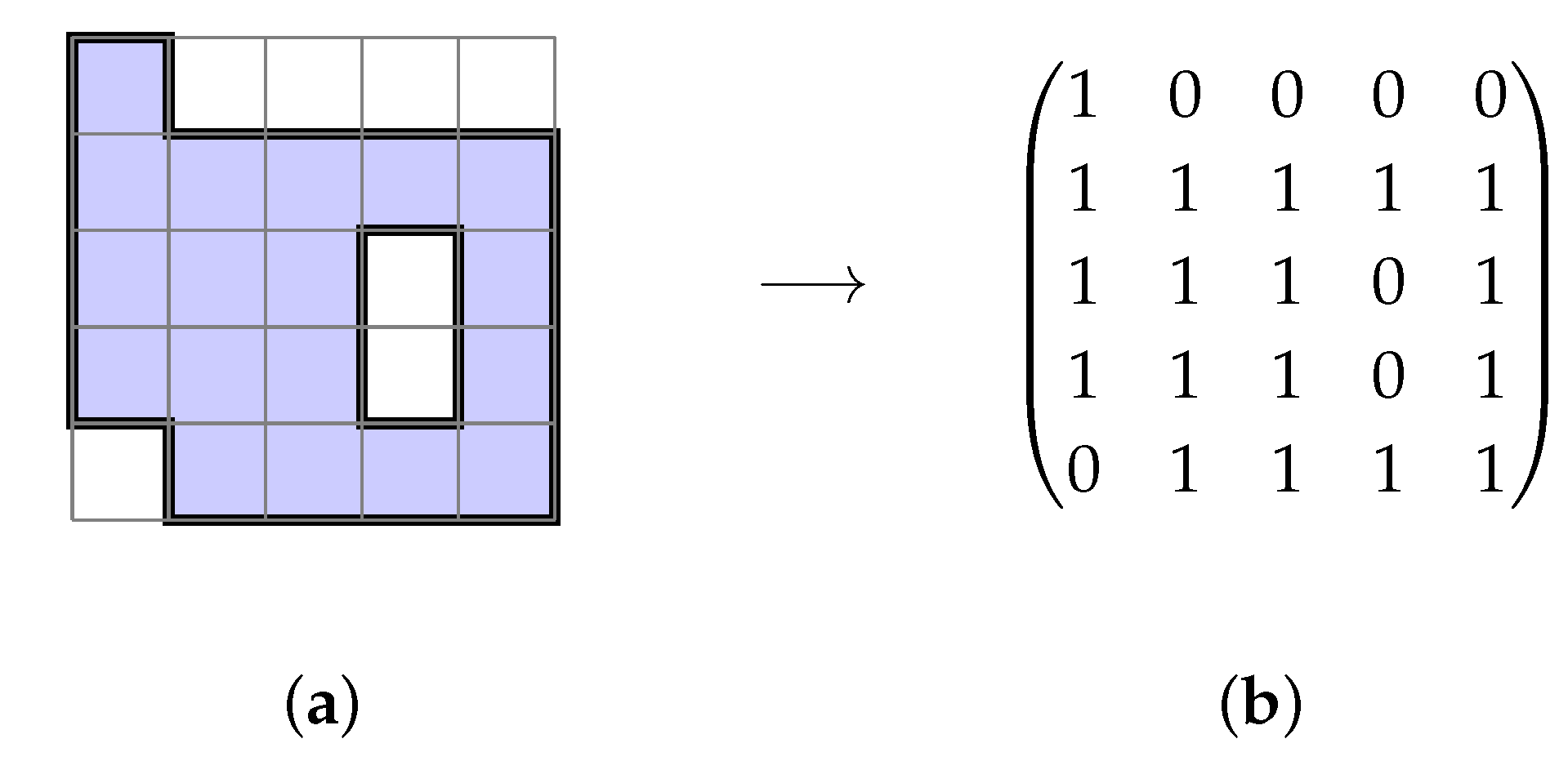
12]. For tiling reasons, we can translate free, one-sided, and fixed polyominoes in a
target region R. We assume the target region is connected, but not necessarily simply connected, i.e., we let
R have ‘holes’. There are two basic tiling situations: tiling with copies of a single free polyomino, or tiling with two or more distinct free polyominoes (with or without copies). We refer to these cases as
monohedral and
multihedral, respectively. For more background theory on polyominoes and tiling with polyominoes, we refer the reader to standard references (see e.g., [
5,
7,
13,
14,
15,
16] and the citations there). There is also a large specialized literature on the many computational and theoretical aspects of tiling the plane with polyominoes [
17,
18,
19,
20,
21,
22,
23], or tiling finite regions of the plane with polyominoes (e.g., [
24,
25,
26,
27,
28,
29,
30,
31,
32,
33,
34,
35,
36,
37,
38,
39,
40]). Unless stated otherwise, in the rest of this article, we assume polyominoes are free.
Tiling with polyominoes is an example of combinatorial optimization [
41,
42]. The key challenge is to develop algorithms that solve large tiling problems in a reasonable amount of time [
43]. The general problem of tiling finite regions of the plane with polyominoes is
-complete [
42,
44,
45], and so the associated computational geometry problem rapidly becomes intractable for large instances. Thus, it is important to reduce algorithm complexity for tiling, and this area continues as a fruitful area of research.
The method in this article for tiling relies on combining two different techniques, namely, integer linear programming (ILP) [
46] and checkerboard colouring techniques [
47]. We give a very simple tiling example to motivate our tiling strategy and leave the formal development of the method and definitions to
Section 3. Although the two solutions are obvious, for the sake of introducing the colouring approach, we proceed as though the solution is unknown, to highlight the issues involved.
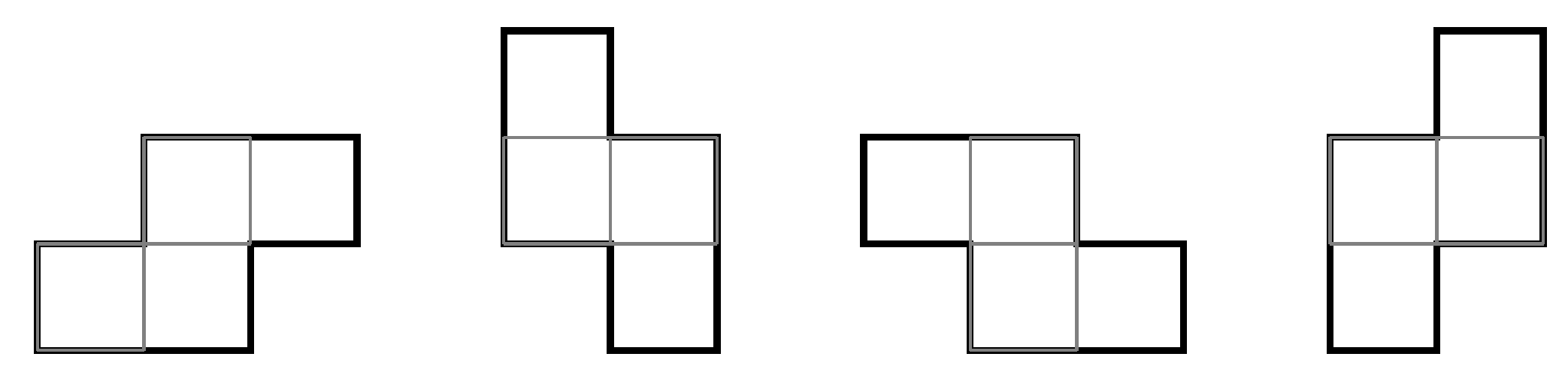
Consider the problem of tiling the
rectangle, denoted
R, with two L-shaped tetrominoes

, all orientations permitted. Initially, we review the basic ILP approach that was developed in [
46] and then solve the same problem with the addition of colouring techniques.
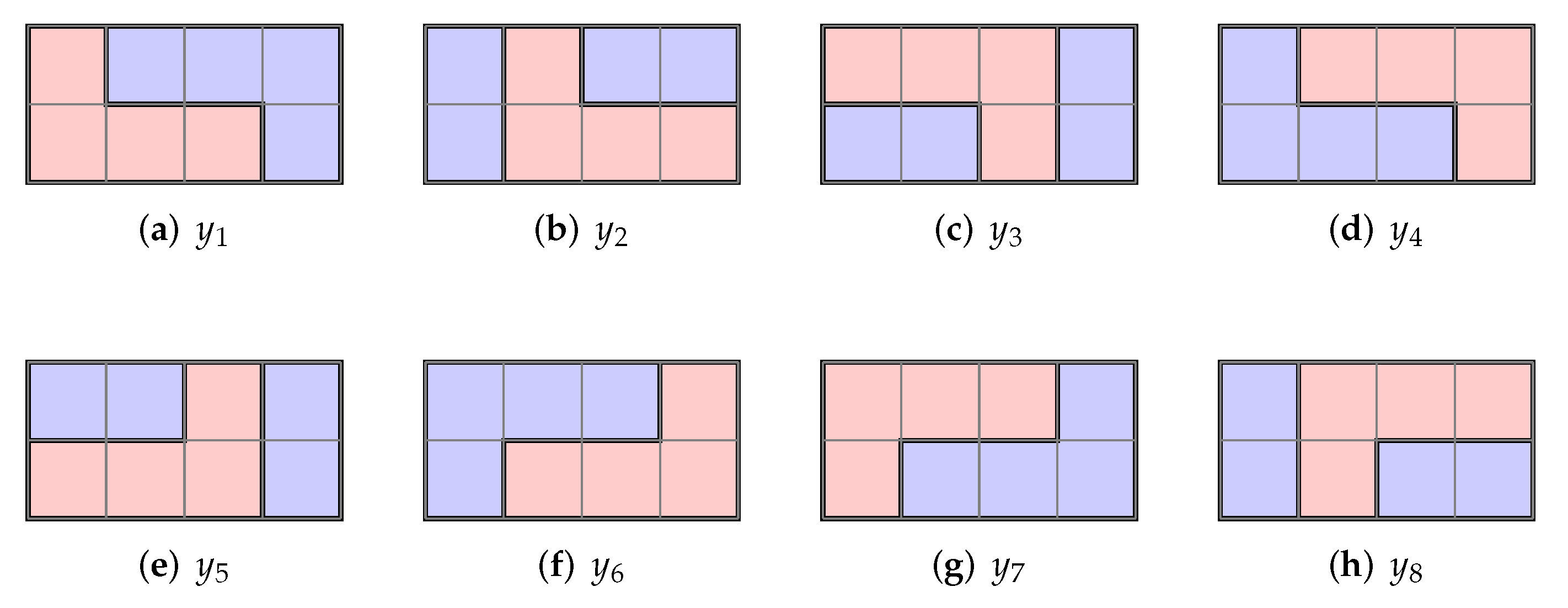
We introduce a variable
for whether we use a particular placement of a tetromino ( coloured red) to tile the region, illustrated in
Figure 1.
In any tiling of
R, we must cover each of the eight cells exactly once, yielding the following system of eight linear equations in eight unknowns:
Observe that if we sum these equations, we obtain
, which implies that we must use exactly two polyominoes to tile the region. Thus, this constraint is automatically incorporated into the system. A tiling of the region
R corresponds to a binary solution of this system. However, solutions of the extended system where
do not necessarily correspond to a tiling as solutions may also be rational. The reduced row echelon form of this system has seven non-zero rows and eight variables, thus one free variable. Solving this system, using a high-performance optimization package, such as
CPLEX,
Gurobi, or
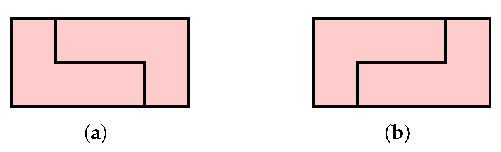
SCIP, yields two binary solutions:
with all other variables equal to zero; and
with all other variables equal to zero, illustrated in
Figure 2. These tilings are trivial variations of each other, obtained by reflecting the entire board horizontally.
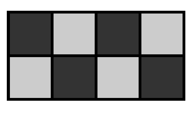
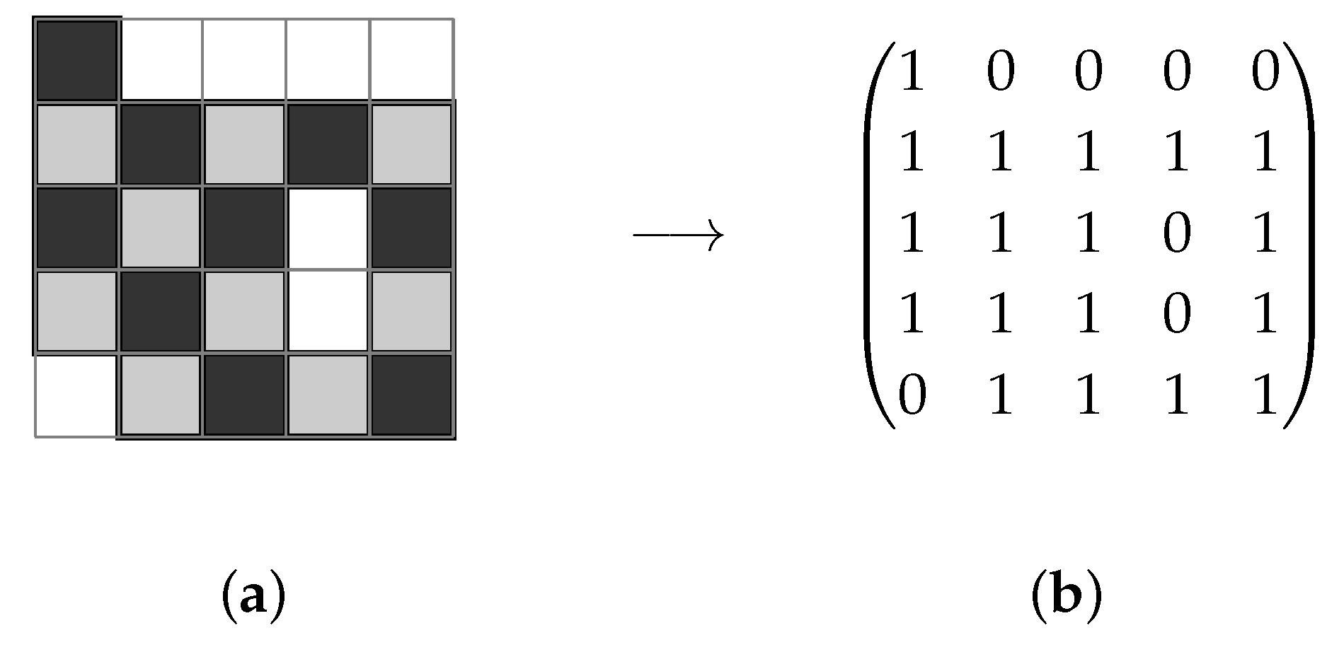
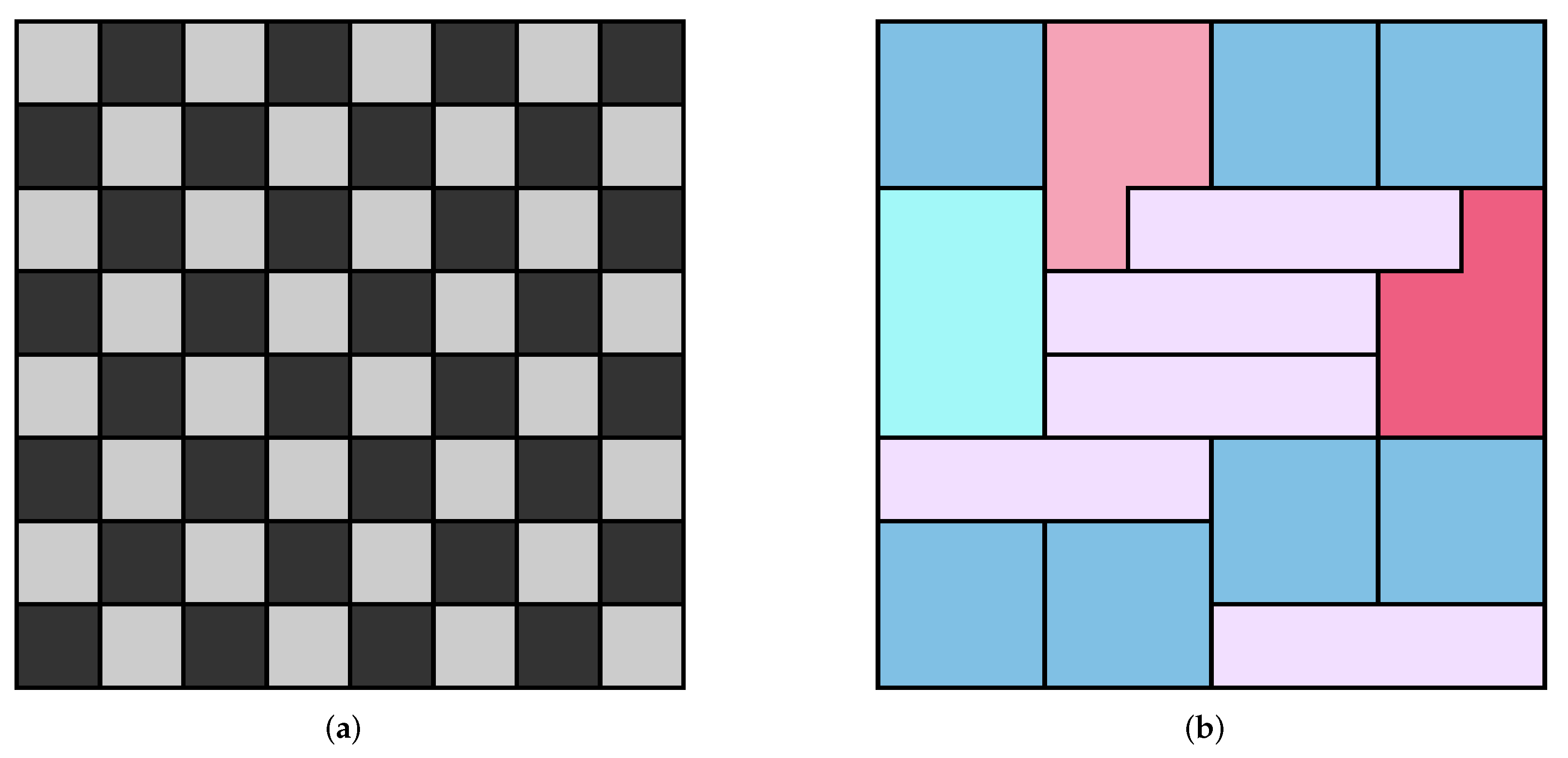
We now solve this tiling problem by including checkerboard colouring techniques. The starting point of the approach is to give the target region
R a fixed checkerboard colouring, illustrated in
Figure 3. There is another checkerboard colouring for this region obtained by swapping the black and white squares, but the particular choice of colouring does not matter to the solution procedure.
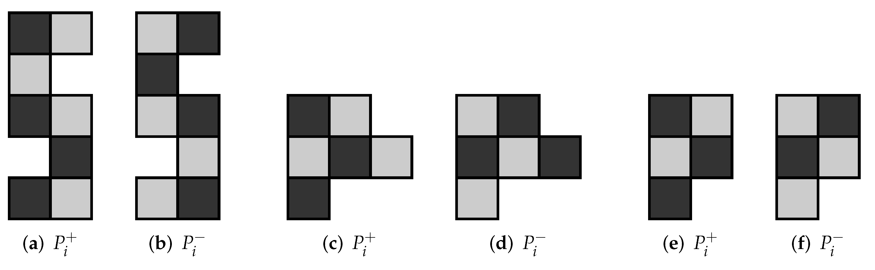
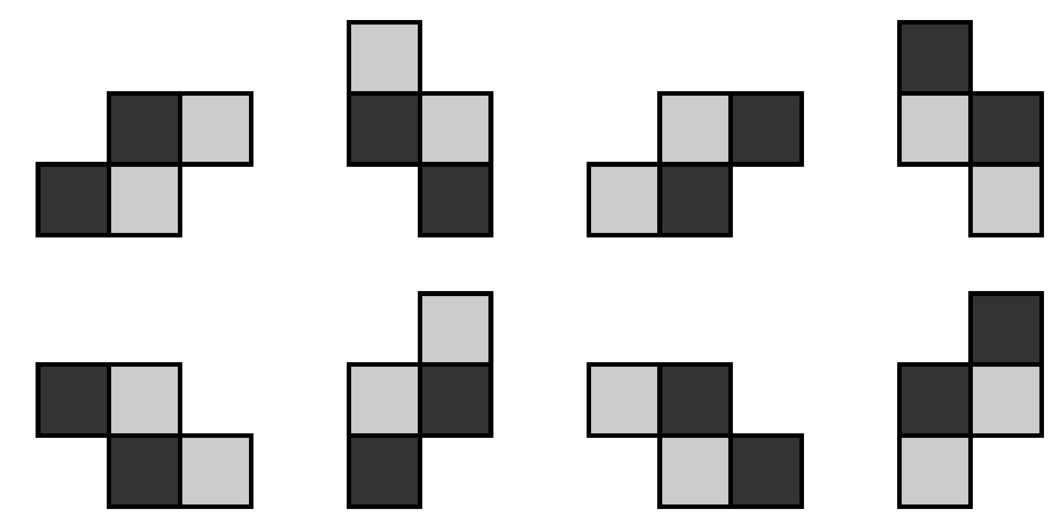
We also assume that the tetrominoes used to tile
R have a checkerboard colouring, and the two distinct variants are

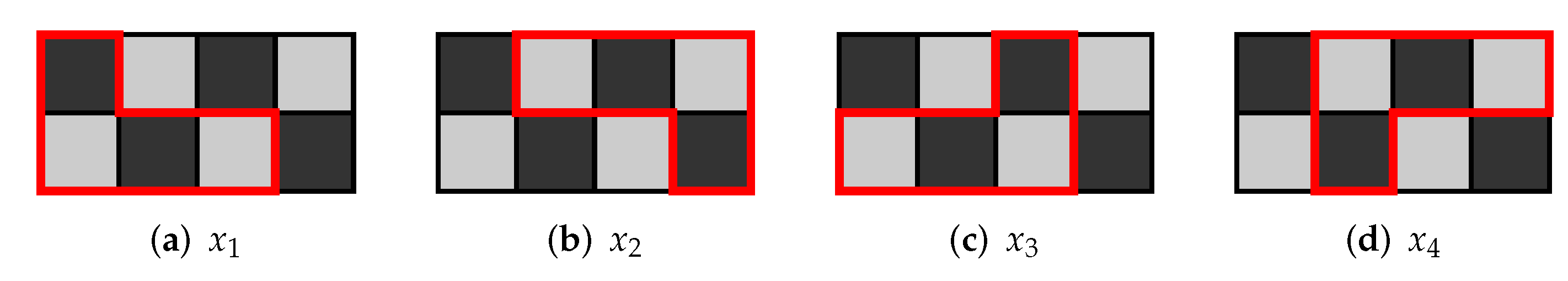
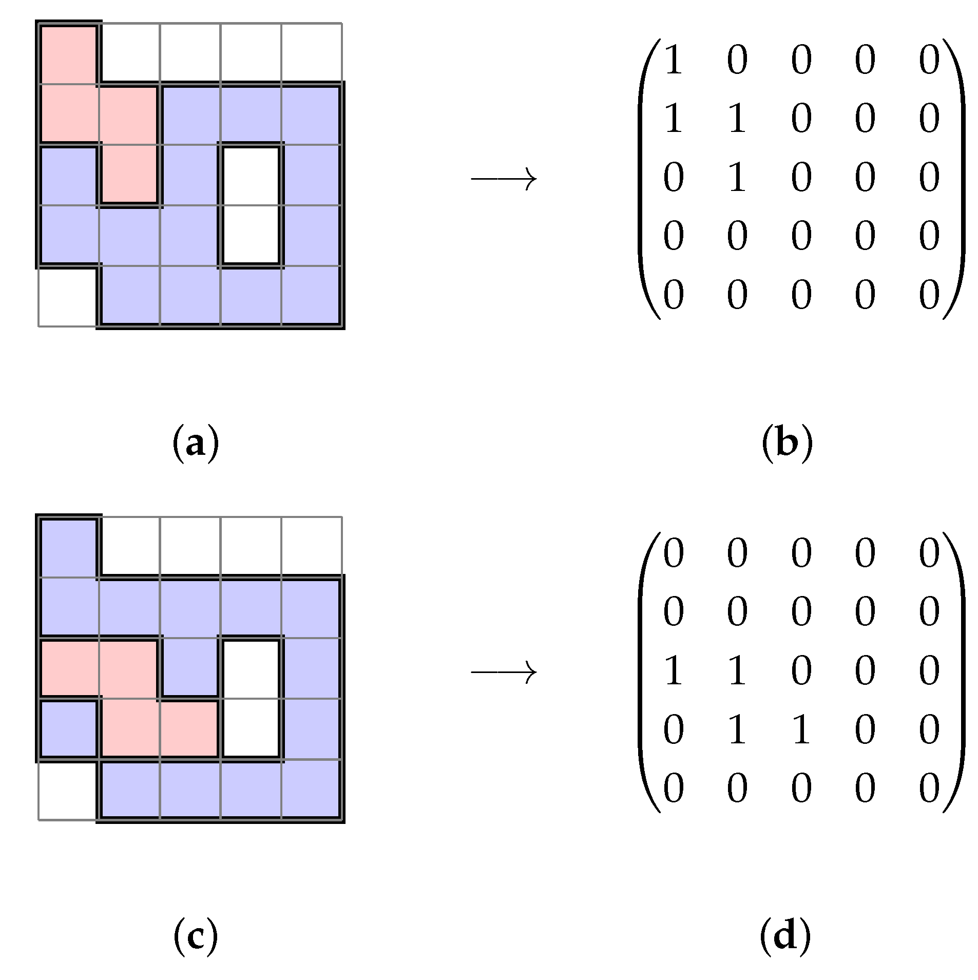
where all orientations are permitted. Not only must the coloured polyominoes fit in the target region, but the colouring of the cells covered must correspond to the colouring of the cells in the tiles. Using two coloured tetrominoes from this set yields three subcases: tiling with two of the first coloured tetromino; tiling with one coloured tetromino of each variant; or tiling with two of the second coloured tetromino. We focus on the first subcase. We introduce a variable
for whether a particular placement of a coloured tetromino of the first kind in this set is used to tile the region, illustrated in
Figure 4.
In any tiling of the checkerboard coloured region in
Figure 3, each of the eight cells must be covered exactly once, yielding the following system of eight linear equations in four unknowns:
If we sum these equations, we obtain
, which again reflects the fact that we must use exactly two coloured polyominoes of the first variant to tile the region. Thus, this constraint is also automatically incorporated into the system. However, unlike in the previous example, this system has full rank and is thus trivially solved to yield
with all other variables equal to zero, i.e., we have the first tiling solution illustrated in
Figure 2. The third subcase is similar, yielding the second tiling solution illustrated in
Figure 2.
In the second subcase, unlike the first and third subcases, we are tiling with two different coloured polyominoes. So each coloured polyomino has an associated constraint equation that must be incorporated into the linear system (i.e., unlike the case with a single polyomino or coloured polyomino, they are not both automatically incorporated into the linear system). This is like the multihedral case for tiling with polyominoes [
46], which we review in the next section. The system of equations arising from the second subcase also has full rank; however, the unique solution of the extended system with
is non-binary, and thus does not correspond to a tiling solution. This tiling example, although very simple, highlights an important point. When we combine checkerboard colouring techniques with the ILP approach for tiling, the problem can split into several subproblems with a reduction in subproblem complexity. Each subproblem is independently solvable, and the solutions to the full problem were partitioned among the subproblems.
The problem we introduced above is very simple, and not only because it is a small monohedral problem. The tetromino we used to tile the region is what we call ‘balanced’, i.e., when we apply a checkerboard colouring to this tile, the number of black cells is equal to the number of white cells. Thus, when tiling a region with
N copies of a balanced tile, there will always be
subcases to consider when seeking all tiling solutions:
r tiles of the second coloured variant with
tiles of the first coloured variant, where
. However, we often tile with checkerboard coloured polyominoes that are not balanced, in which case the splitting of the full problem into subproblems depends on the ‘parity’ of the tiles and the target region, where we define parity as the number of black squares minus the number of white squares of a tile or region (see the next section and [
47]).
1.2. Goals and Related Work
The traditional approach to tiling finite regions of the plane with polyominoes employs backtracking, which is the default way in computer science for exploring the search tree of a combinatorial problem [
48,
49,
50,
51,
52]. Although backtracking is quick for some problems, it only refines a ‘brute-force’ solution procedure for exhaustively finding all solutions to a combinatorial search problem. Another less commonly used ‘brute-force’ approach to tiling with polyominoes employs either evolutionary computation [
26] or genetic algorithms [
53]; however, such approaches are likely considerably less efficient than backtracking. The only other general-purpose algorithmic procedure to tiling finite regions of the plane with polyominoes that we are aware of uses ILP, first introduced in [
46]. There are several potential advantages of an algebraic approach to tiling over the backtracking methods. In [
46], the authors note that with ILP the “the structure, combinatorial nature, and solvability of the model can be analyzed”. Finally, we mention there are many pure mathematical results for proving that a set of polyominoes tiles a region, for example, using the combinatorial group theory approach of J.H. Conway [
54,
55,
56]. However, these methods typically apply only to special cases and thus, we cannot make them algorithmic.
It is interesting to note that the tiling problem, which is here regarded as an ILP instance, can also be considered a satisfiability problem (SAT) [
57,
58,
59], for which there are a number of powerful solvers. Examples of suitable open-source SAT solvers include
Lingeling; see
http://fmv.jku.at/lingeling/ (accessed on 20 March 2022) and
MapleSAT, see
https://sites.google.com/a/gsd.uwaterloo.ca/maplesat/maplesat (accessed on 20 March 2022). Unfortunately, however, the overhead of enforcing the conditions that we use each tile a fixed number of times is prohibitive. Further details are provided in
Appendix A.
The focus of the current article is to combine checkerboard colouring techniques adapted from [
47] with a recently introduced ILP method [
46] for tiling with polyominoes. The checkerboard colouring method [
47] was originally used to identify large impossible tiling problems, i.e., the opposite of what we aim to do here. Our checkerboard colouring techniques often splits large tiling problems into smaller tiling subproblems, where each subproblem is represented as a separate ILP problem. Problems that are amenable to this approach are embarrassingly parallel. This article provides proof of concept of a parallelizable ILP approach for tiling finite regions of the plane with polyominoes. We construct the ILP formulations of the tiling problems in
MATLAB and compute the numerical solutions using
CPLEX, a high-performance optimization package. The primary goal is to analyze when this approach yields a potential parallel speedup.
For tiling problems solved via a parallelizable ILP optimization technique, there are two basic aims: (i) find a single tiling solution (i.e., an optimal solution), and (ii) find all tiling solutions. In the former case, when we apply our checkerboard colouring techniques, we seek the subcase yielding an optimal solution computed in the least amount of time. In the latter case, it is the subcase that takes the longest time to compute all solutions that is of interest; if this takes less time to compute than for the full (uncoloured) problem, then we have a potential parallel speedup.
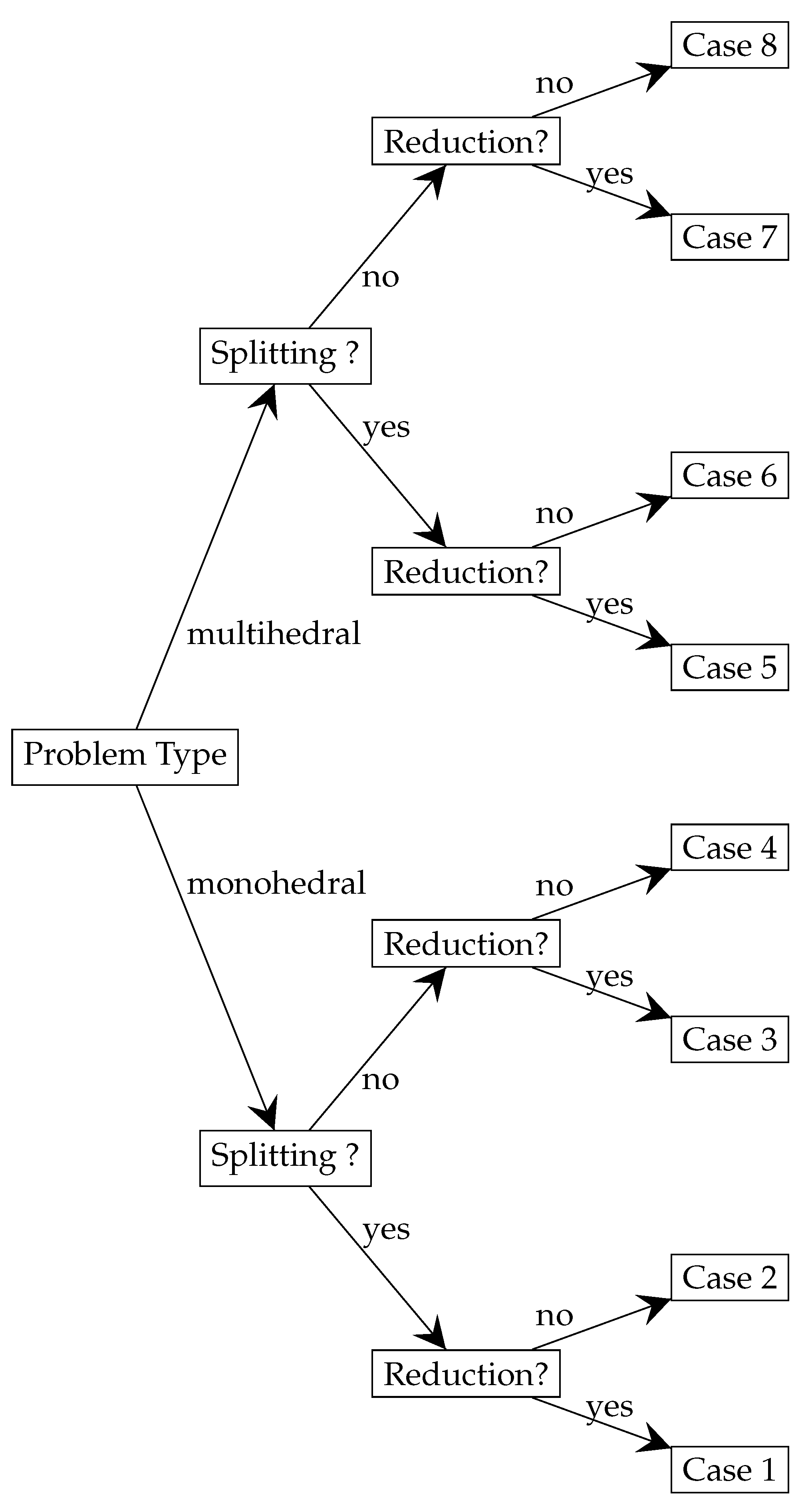
The simple tiling examples discussed above raise many questions, namely the following:
When do the checkerboard colouring techniques split the problem into multiple (≥2) independently solvable subproblems?
For large problems (a large target region and/or the use of many tiles), what is an appropriate measure of problem complexity and the work done to compute tiling solutions?
Under what situations does this ‘splitting’ technique yield a potential parallel speedup with parallel computing?
We structure the remaining parts of this article as follows. After giving some preliminary details about checkerboard colouring in
Section 2, we describe how to build the ILP model formulation for tiling in
Section 3. In
Section 4, we describe how large tiling problems often split into many smaller tiling subproblems with the application of checkerboard colouring techniques.
Section 5 deals with the theoretical issues of complexity, measures of performance, and problem classification.
Section 6 presents the numerical solution of medium to large tiling problems, and in
Section 7 we make some general comments about algorithm performance. Concluding remarks are in
Section 8. Finally, in
Appendix A, we discuss the possible application of an SAT solver to our tiling problem.


 , all orientations permitted. Initially, we review the basic ILP approach that was developed in [46] and then solve the same problem with the addition of colouring techniques.
 where all orientations are permitted. Not only must the coloured polyominoes fit in the target region, but the colouring of the cells covered must correspond to the colouring of the cells in the tiles. Using two coloured tetrominoes from this set yields three subcases: tiling with two of the first coloured tetromino; tiling with one coloured tetromino of each variant; or tiling with two of the second coloured tetromino. We focus on the first subcase. We introduce a variable for whether a particular placement of a coloured tetromino of the first kind in this set is used to tile the region, illustrated in Figure 4.
 all orientations permitted. The area of R is 80, so we need 20 copies of the L-shaped tetromino. The associated binary ILP file, constructed with the program LPMAKE_POLYOMINOES_FIGURE2, has n = 442 unknowns, m = 80 constraints, and f = 363 free variables. CPLEX
found 1,709,594 solutions in 367.9 s.
all orientations permitted. The area of R is 80, so we need 20 copies of the L-shaped tetromino. The associated binary ILP file, constructed with the program LPMAKE_POLYOMINOES_FIGURE2, has n = 442 unknowns, m = 80 constraints, and f = 363 free variables. CPLEX
found 1,709,594 solutions in 367.9 s. all orientations permitted.

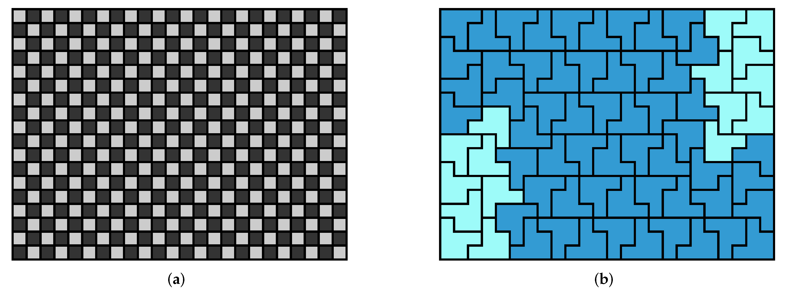
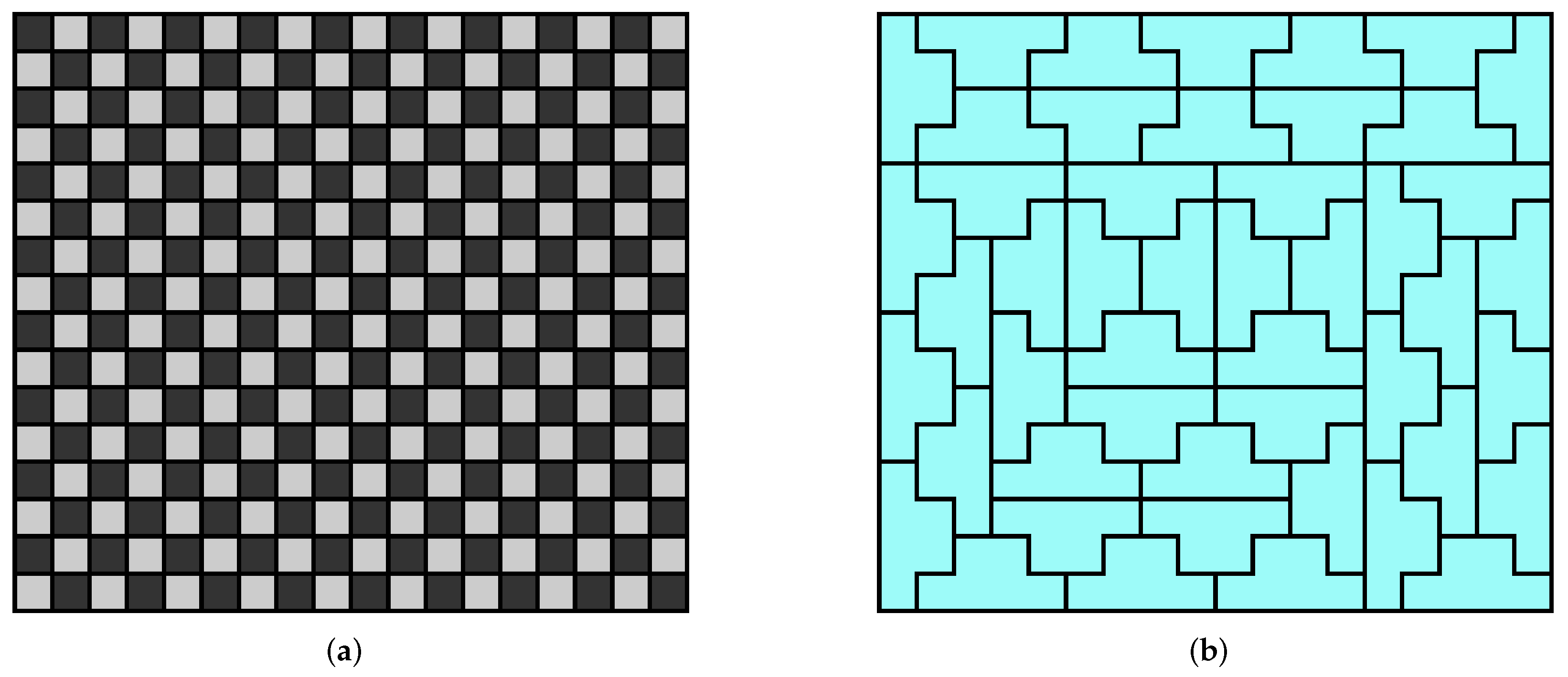
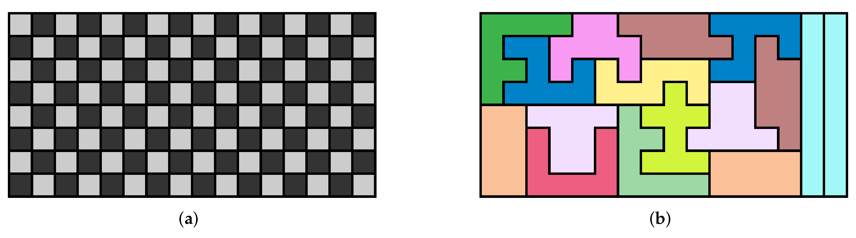
 all orientations permitted. The area of R is 432, so we need 72 copies of the hexomino. The associated ILP file, constructed with the program LPMAKE_POLYOMINOES_FIGURE3, has n = 2816 unknowns, m = 432 constraints, and f = 2385 free variables. CPLEX found 414 solutions in s.
 all orientations permitted.
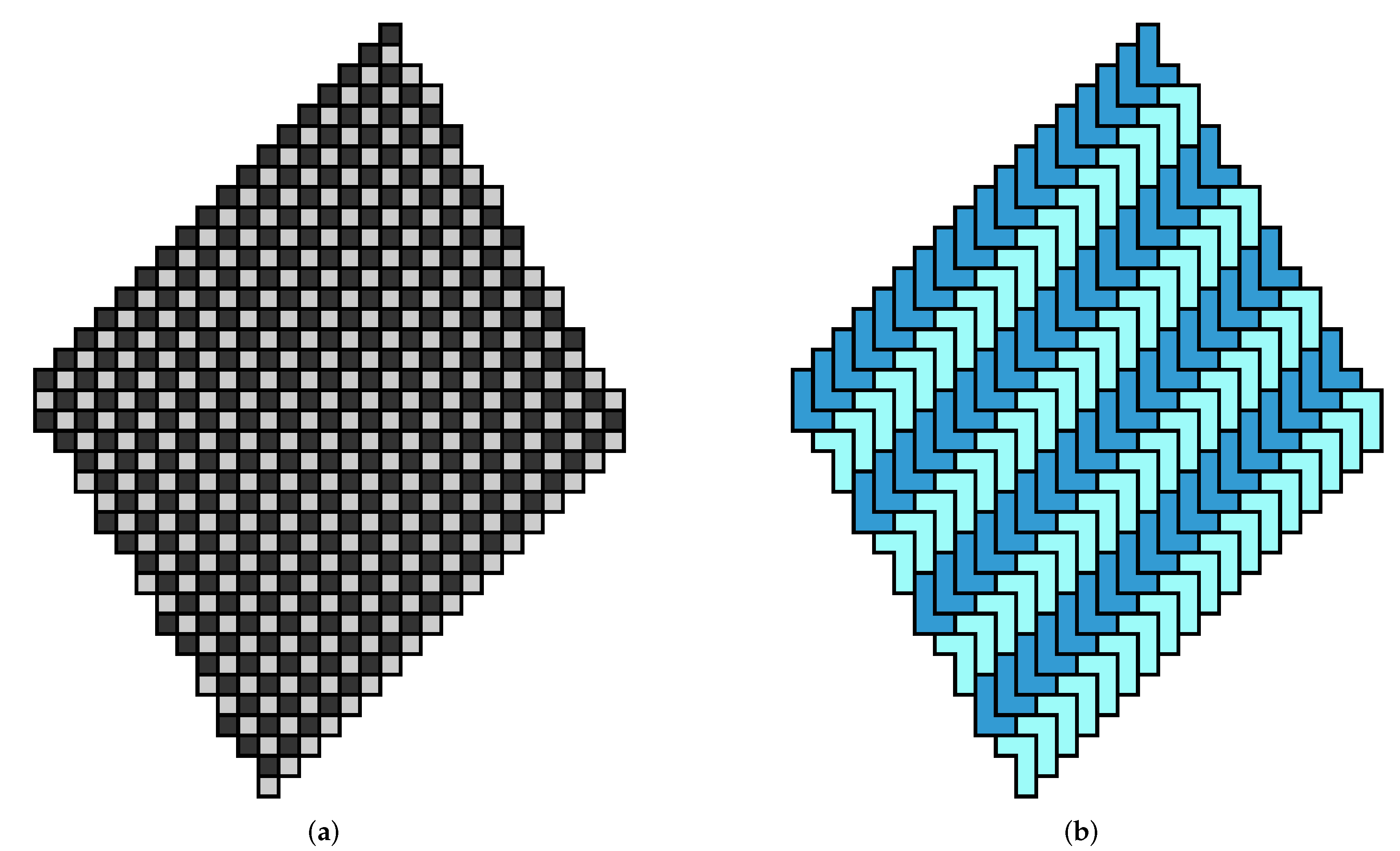
 all orientations permitted. The area of R is 576, so we need 144 copies of the L-shaped tetromino. The associated ILP file, constructed with the program LPMAKE_POLYOMINOES_FIGURE4, has n = 3952 unknowns, m = 576 constraints, and f = 3377 free variables. CPLEX found a single solution in 0.15 s.
 all orientations permitted.
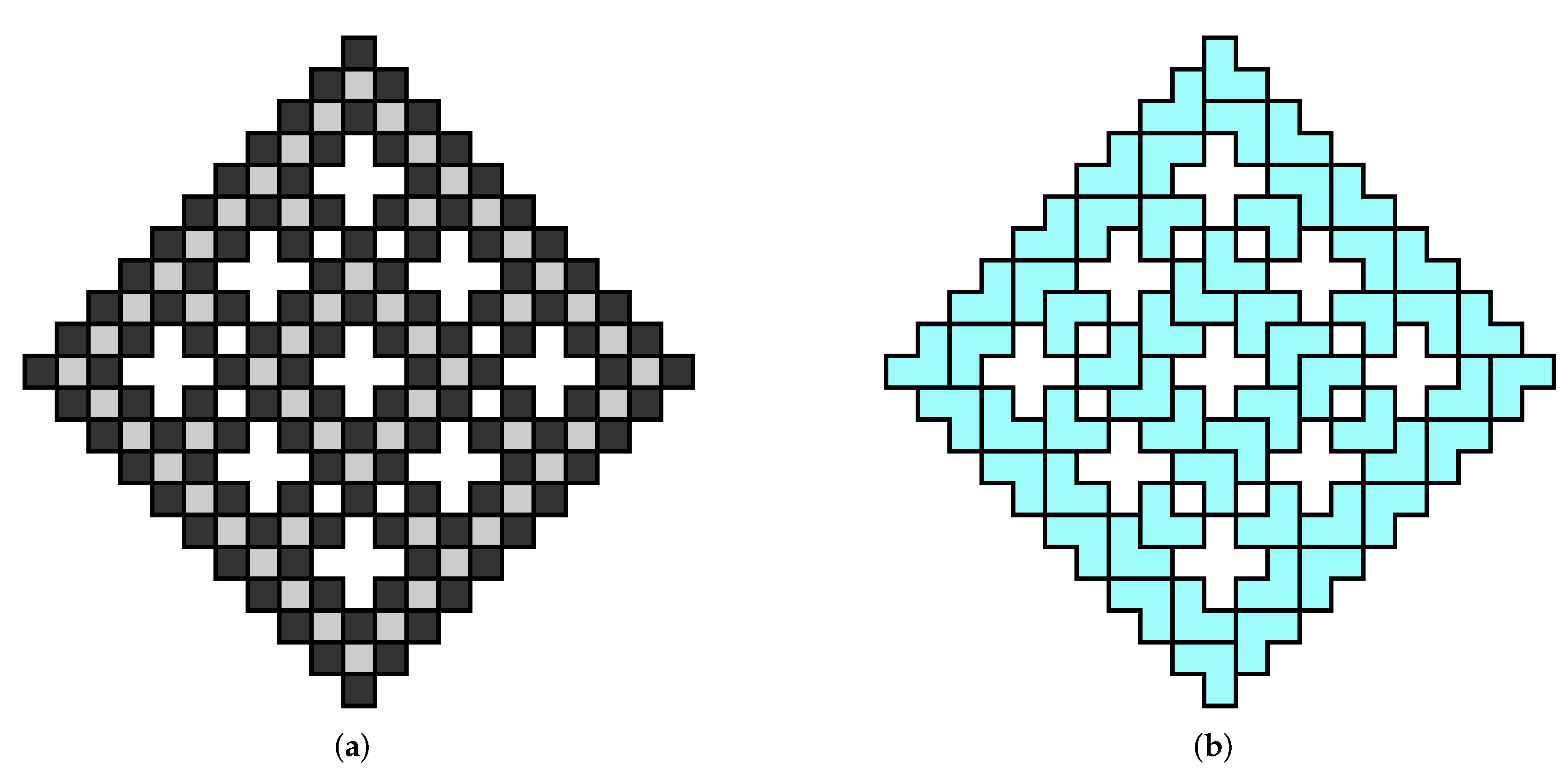
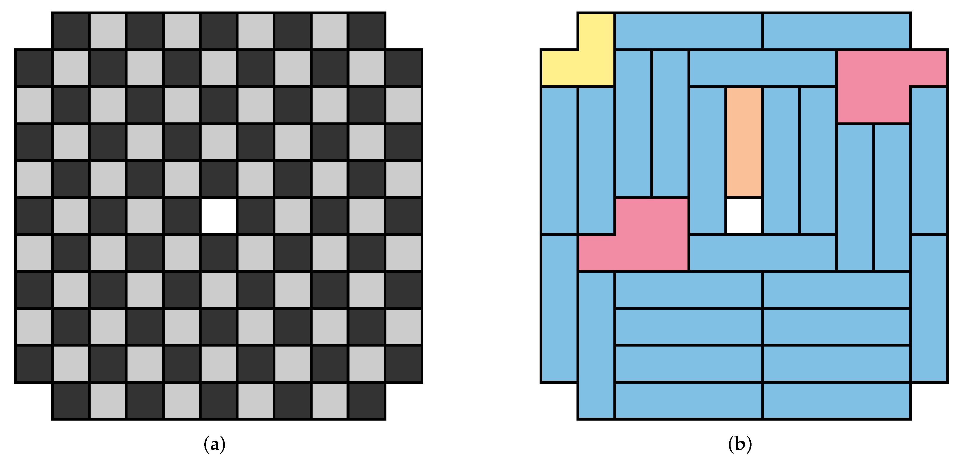
 all orientations permitted. The area of R is 168, so we need 56 copies of the L-shaped trimino. The associated ILP file, constructed with the program LPMAKE_POLYOMINOES_FIGURE5, has n = 336 unknowns, m = 168 constraints, and f = 168 free variables. CPLEX found 16 solutions in 0.05 s.
 with parities , all orientations permitted. The parity of is , thus the only way to satisfy the parity equation (see Theorem 1) is to choose and . That is, the only way to tile is to use the pariominoes and we have a single pariomino tiling subproblem. We constructed the ILP file using the program LPMAKE_PARIOMINOES_FIGURE5. CPLEX found 16 solutions with in 0.02 s, thus the potential speedup when using the colouring technique is about 2.5×. However, as the runtimes are very small, this is not a particularly meaningful measure. The optimal solution of the pariomino tiling subproblem is shown in Figure 16b.
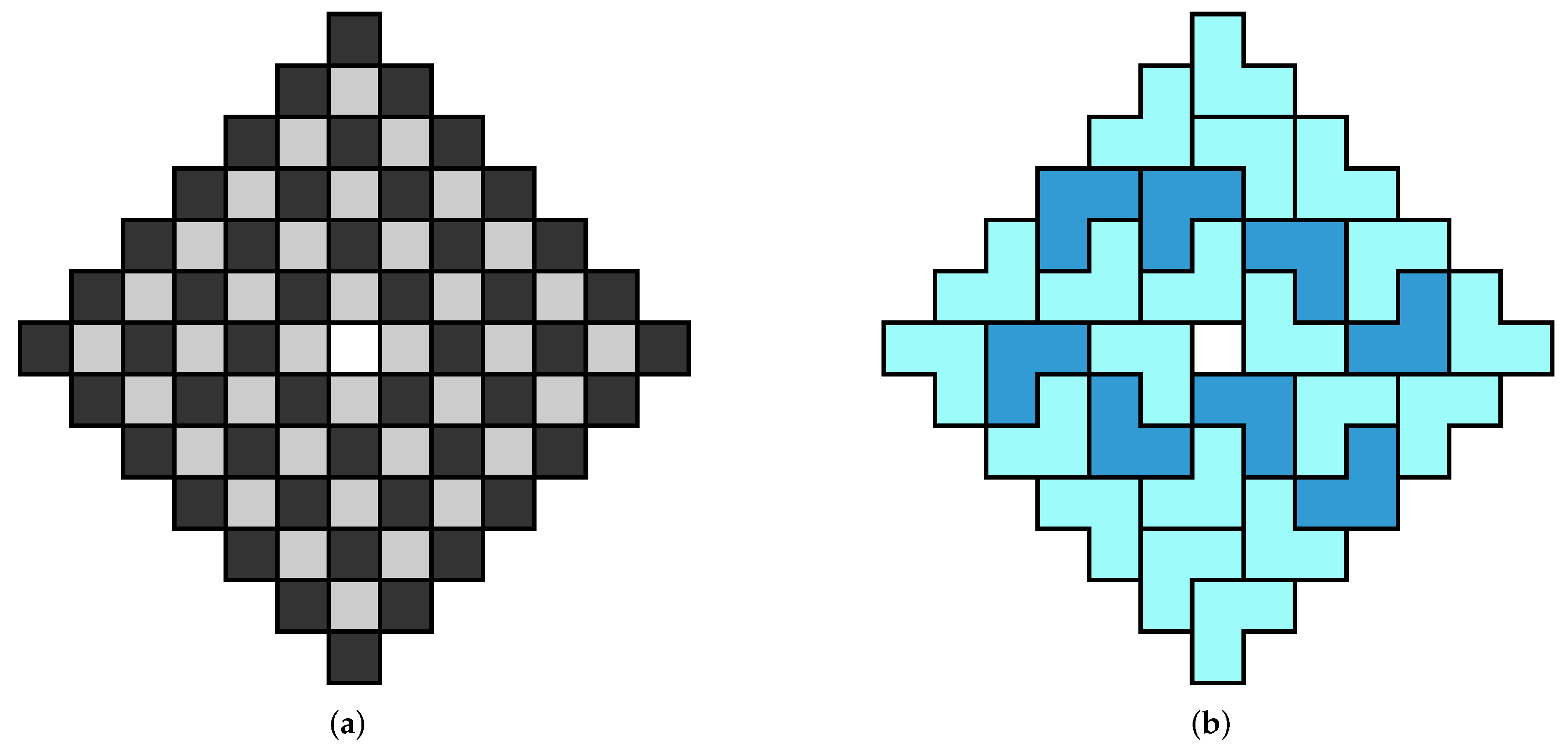
 all orientations permitted. The area of R is 84, so we need 28 copies of the L-shaped trimino. The associated ILP file, constructed with the programLPMAKE_POLYOMINOES_FIGURE6, has n = 252 unknowns, m = 84 constraints, and f = 168 free variables.CPLEX found 731,092 solutions in 165.78 s.
 with parities , all orientations permitted. The parity of is , thus, the only way to satisfy the parity equation (see Theorem 1) is to choose and , i.e., we have a single pariomino tiling subproblem using 20 copies of and 8 copies of . The ILP file was constructed using the program LPMAKE_PARIOMINOES_FIGURE6. Solving this subproblem in CPLEX yielded 731,092 solutions with in 156.20 s, thus the potential speedup when using the colouring technique is about 1.1×. The optimal solution of the pariomino tiling subproblem is shown in Figure 17b.
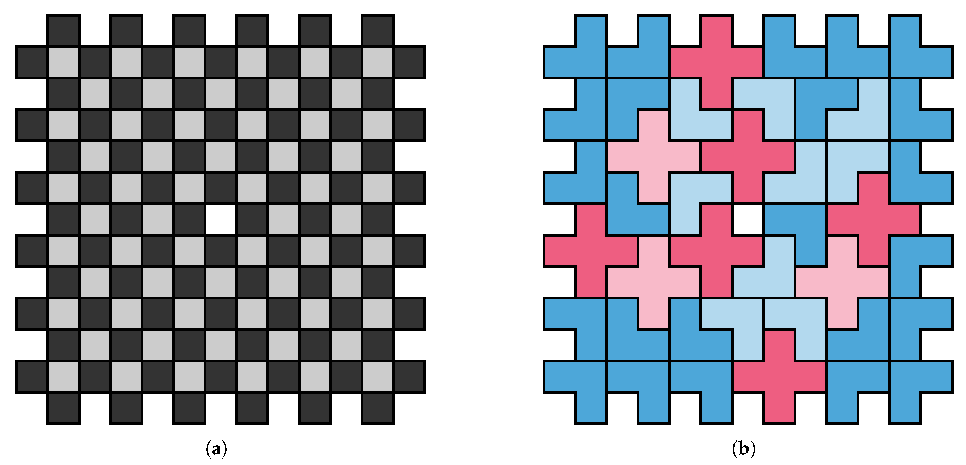
 all orientations permitted. The area of R is 288, so we need 48 copies of the hexomino. The associated ILP file, constructed with the program LPMAKE_POLYOMINOES_FIGURE7, has n = 892 unknowns, m = 288 constraints, and f = 609 free variables. CPLEX found 217,266 solutions in 45.55 s.
 all orientations permitted. We note here thatand so we only tile with copies of a single pariomino.
 all orientations permitted. The area of R is 144, which we aim to tile using= 33 copies of an L-shaped trimino and= 9 copies of the cross-shaped pentomino. The associated ILP file, constructed with the program
LPMAKE_POLYOMINOES_FIGURE8, has n = 528 unknowns, m = 146 constraints, and f = 383 free variables.
CPLEX
found 731,092 solutions in 165.78 s.
all orientations permitted. The area of R is 144, which we aim to tile using= 33 copies of an L-shaped trimino and= 9 copies of the cross-shaped pentomino. The associated ILP file, constructed with the program
LPMAKE_POLYOMINOES_FIGURE8, has n = 528 unknowns, m = 146 constraints, and f = 383 free variables.
CPLEX
found 731,092 solutions in 165.78 s. with parities, and 9 pariominoes from the set
 with parities, all orientations permitted. The parity equation (see Theorem 1) is given by
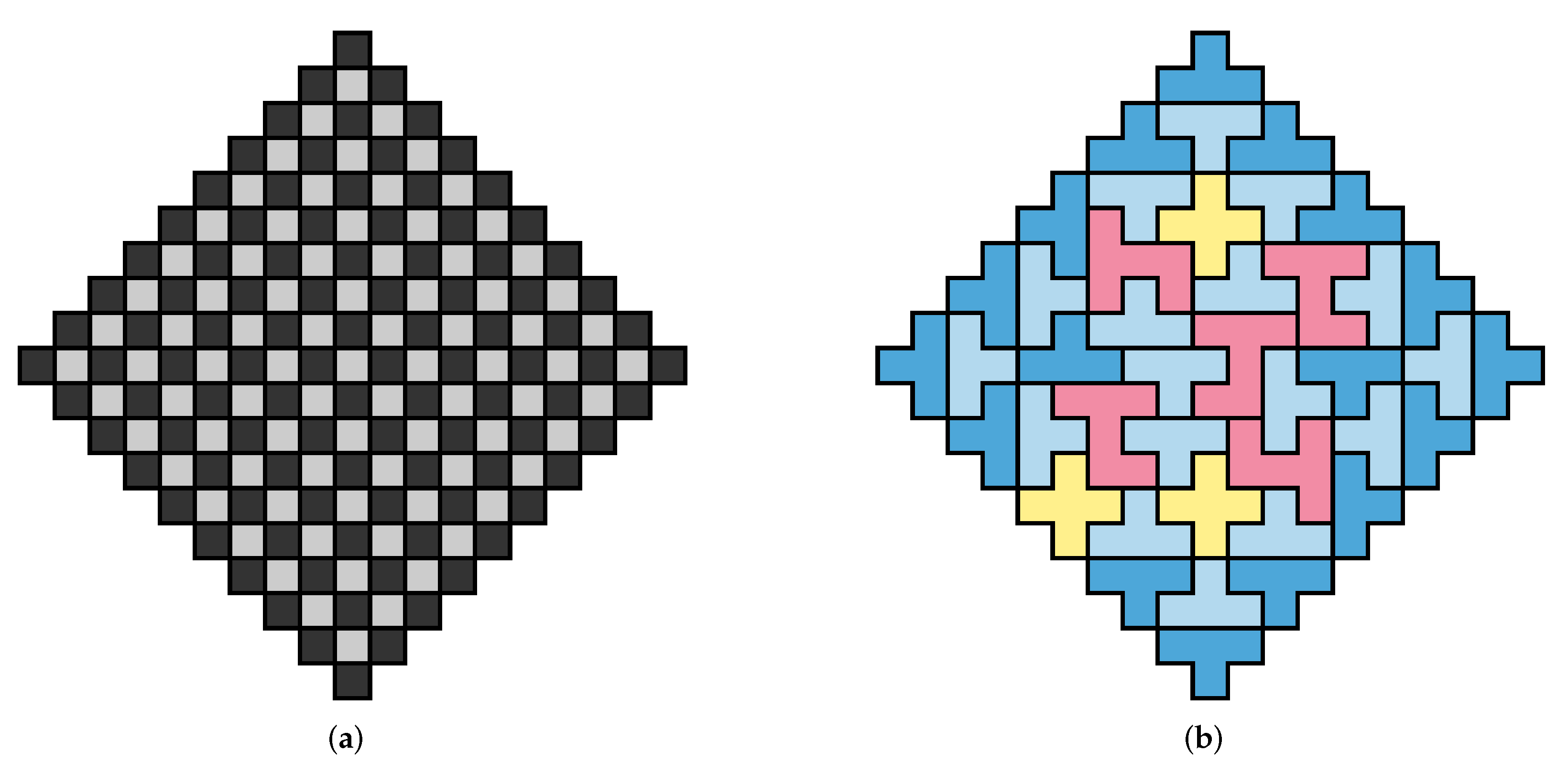
 all orientations permitted. The area of R is 181, which we aim to tile using= 34 copies of the T-shaped trimino,= 5 copies of Y-shaped hexomino, and= 3 copies of the cross-shaped pentomino. The ILP file, constructed with the program
LPMAKE_POLYOMINOES_FIGURE9, has n = 1685 unknowns, m = 184 constraints, and f = 1502 free variables.
CPLEX
found 337,680 solutions in 225.06 s.
all orientations permitted. The area of R is 181, which we aim to tile using= 34 copies of the T-shaped trimino,= 5 copies of Y-shaped hexomino, and= 3 copies of the cross-shaped pentomino. The ILP file, constructed with the program
LPMAKE_POLYOMINOES_FIGURE9, has n = 1685 unknowns, m = 184 constraints, and f = 1502 free variables.
CPLEX
found 337,680 solutions in 225.06 s. with parities, and 5 pariominoes from the set
 with parities, and 3 pariominoes from the set
 with parities, all orientations permitted. The parity equation (see Theorem 1) is given by
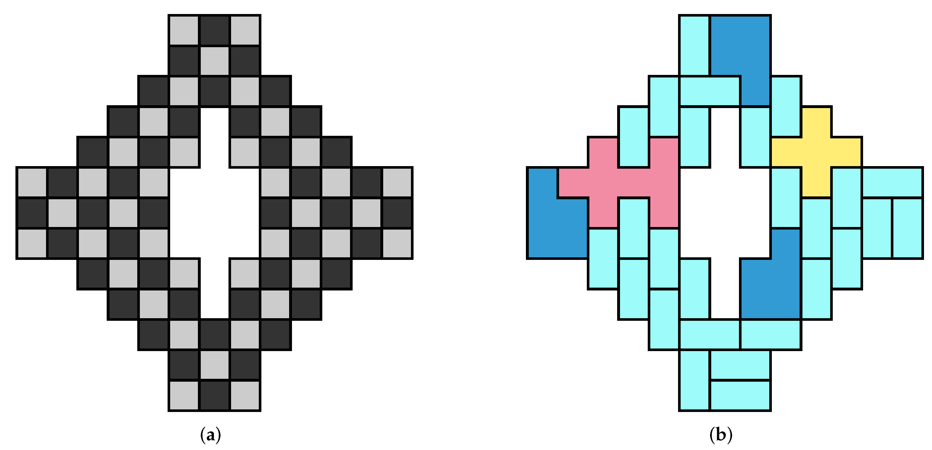
 all orientations permitted. The area of R is 80, which we aim to tile with= 26 copies of the domino,= 3 copies of the P-shaped pentomino,= 1 copies of the cross-shaped pentomino, and= 1 copies of the octomino. The associated ILP file, constructed with the program
LPMAKE_POLYOMINOES_FIGURE10, has n = 444 unknowns, m = 84 constraints, and f = 361 free variables.
CPLEX
found 105,344 solutions in 16.83 s.
all orientations permitted. The area of R is 80, which we aim to tile with= 26 copies of the domino,= 3 copies of the P-shaped pentomino,= 1 copies of the cross-shaped pentomino, and= 1 copies of the octomino. The associated ILP file, constructed with the program
LPMAKE_POLYOMINOES_FIGURE10, has n = 444 unknowns, m = 84 constraints, and f = 361 free variables.
CPLEX
found 105,344 solutions in 16.83 s. with parity, (), and three pariominoes from the set
 with parities, and one pariomino from the set
 with parities, and one pariomino from the set
 with parities, all orientations permitted.
 all orientations permitted, with the following numbers of copies:
 all orientations permitted, wherefor i = 1, 2, …, 7 andfor j = 8, 9, 10. The parities of the pariominoes are given by
 all orientations permitted. The area of R is 116, which we aim to tile using= 25 copies of the straight tetromino,= 1 copy of the straight trimino,= 1 copy of the L-shaped trimino, and= 2 copies of the P-shaped pentomino. The associated ILP file, constructed with the program LPMAKE_POLYOMINOES_FIGURE12, has n = 1376 unknowns, m = 120 constraints, and f = 1257 free variables.
CPLEX
found 429,800 solutions in 768.74 s.
all orientations permitted. The area of R is 116, which we aim to tile using= 25 copies of the straight tetromino,= 1 copy of the straight trimino,= 1 copy of the L-shaped trimino, and= 2 copies of the P-shaped pentomino. The associated ILP file, constructed with the program LPMAKE_POLYOMINOES_FIGURE12, has n = 1376 unknowns, m = 120 constraints, and f = 1257 free variables.
CPLEX
found 429,800 solutions in 768.74 s. with parity, (), and one pariomino from the set
 with parities, and one pariomino from the set
 with parities, and two pariomino from the set
 with parities, all orientations permitted. As the parity ofis, the only way to satisfy the parity equation (see Theorem 1) is to choose 25 copies of(=), one copy of, one copy of, and two copies of. We constructed the ILP file in this case using the program
LPMAKE_PARIOMINOES_FIGURE12. Solving this single subproblem in
CPLEX
withyielded 429,800 solutions in 156.46 s, thus the potential speedup when using the colouring technique is about 4.9×. An optimal solution of this pariomino tiling subproblem is illustrated in Figure 23b.
with parities, all orientations permitted. As the parity ofis, the only way to satisfy the parity equation (see Theorem 1) is to choose 25 copies of(=), one copy of, one copy of, and two copies of. We constructed the ILP file in this case using the program
LPMAKE_PARIOMINOES_FIGURE12. Solving this single subproblem in
CPLEX
withyielded 429,800 solutions in 156.46 s, thus the potential speedup when using the colouring technique is about 4.9×. An optimal solution of this pariomino tiling subproblem is illustrated in Figure 23b.
 all orientations permitted. We aim to tile R using= 5 copies of the straight tetromino,= 7 copies of the 2 × 2 square,= 1 copies of the 2 × 3 rectangle, and= 2 copies of the P-shaped pentomino. The ILP file, constructed with the program
LPMAKE_POLYOMINOES_FIGURE13, has n = 549 unknowns, m = 68 constraints, and f = 482 free variables.
CPLEX
found 157,288 solutions in 78 s.
all orientations permitted. We aim to tile R using= 5 copies of the straight tetromino,= 7 copies of the 2 × 2 square,= 1 copies of the 2 × 3 rectangle, and= 2 copies of the P-shaped pentomino. The ILP file, constructed with the program
LPMAKE_POLYOMINOES_FIGURE13, has n = 549 unknowns, m = 68 constraints, and f = 482 free variables.
CPLEX
found 157,288 solutions in 78 s. with parity, (), and seven pariominoes from the set
 with parities, (), and one pariomino from the set
 with parities, (), and two pariominoes from the set
 with parities, all orientations permitted. As the parity ofis zero, the only way to satisfy the parity equation (see Theorem 1) is to choose five copies of(=), seven copies of(=), one copy of(=), and one copy each ofand. We constructed the ILP file in this case using the program
LPMAKE_PARIOMINOES_FIGURE13. Solving this single subproblem in
CPLEX
withyielded 157,288 solutions in 85.3 s, which is an increase in the runtime of about 9.4% compared to the full (uncoloured) tiling problem. Thus, no potential speedup is observed. An optimal solution of this pariomino tiling subproblem is illustrated in Figure 24b.
with parities, all orientations permitted. As the parity ofis zero, the only way to satisfy the parity equation (see Theorem 1) is to choose five copies of(=), seven copies of(=), one copy of(=), and one copy each ofand. We constructed the ILP file in this case using the program
LPMAKE_PARIOMINOES_FIGURE13. Solving this single subproblem in
CPLEX
withyielded 157,288 solutions in 85.3 s, which is an increase in the runtime of about 9.4% compared to the full (uncoloured) tiling problem. Thus, no potential speedup is observed. An optimal solution of this pariomino tiling subproblem is illustrated in Figure 24b.
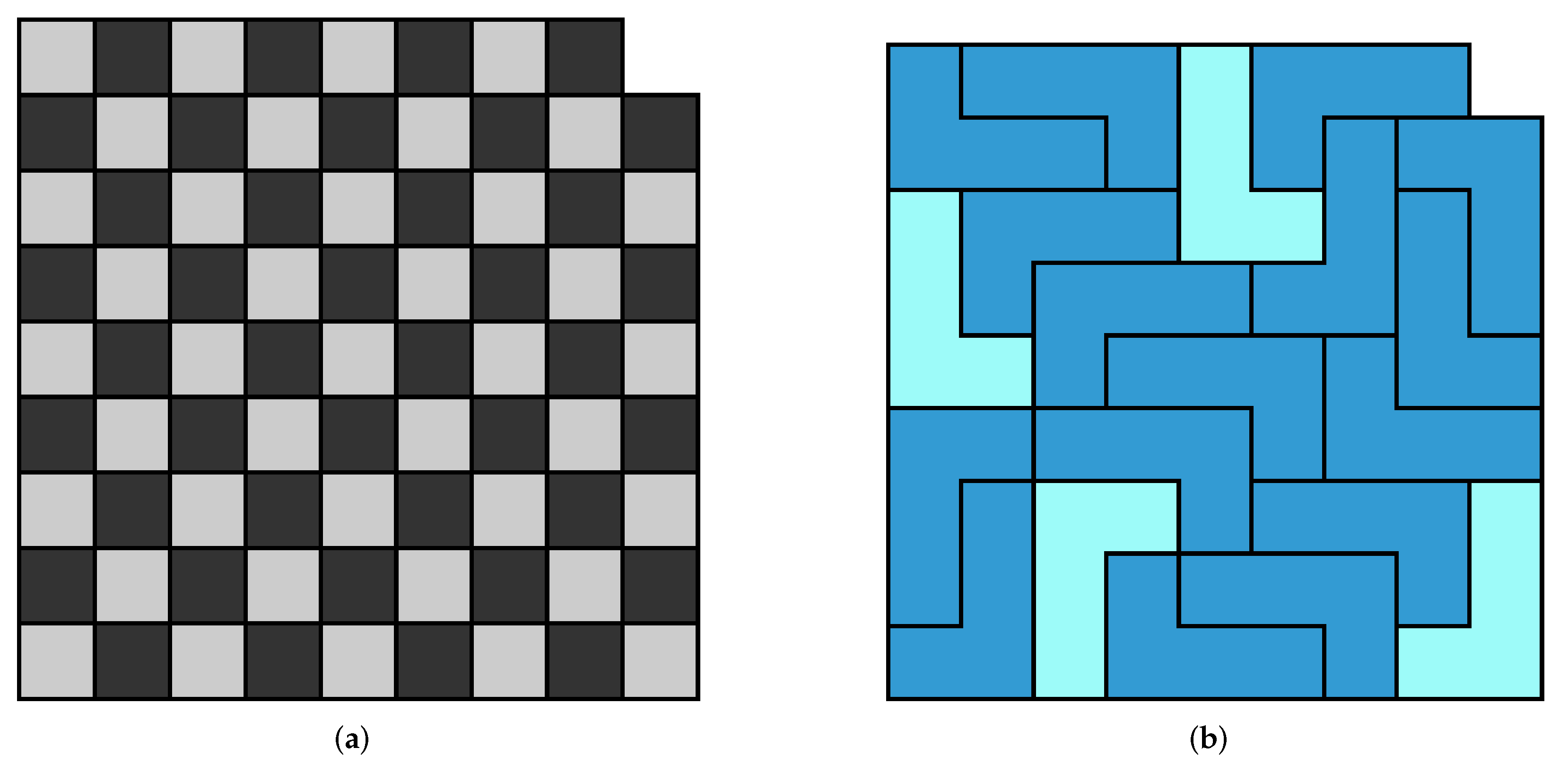
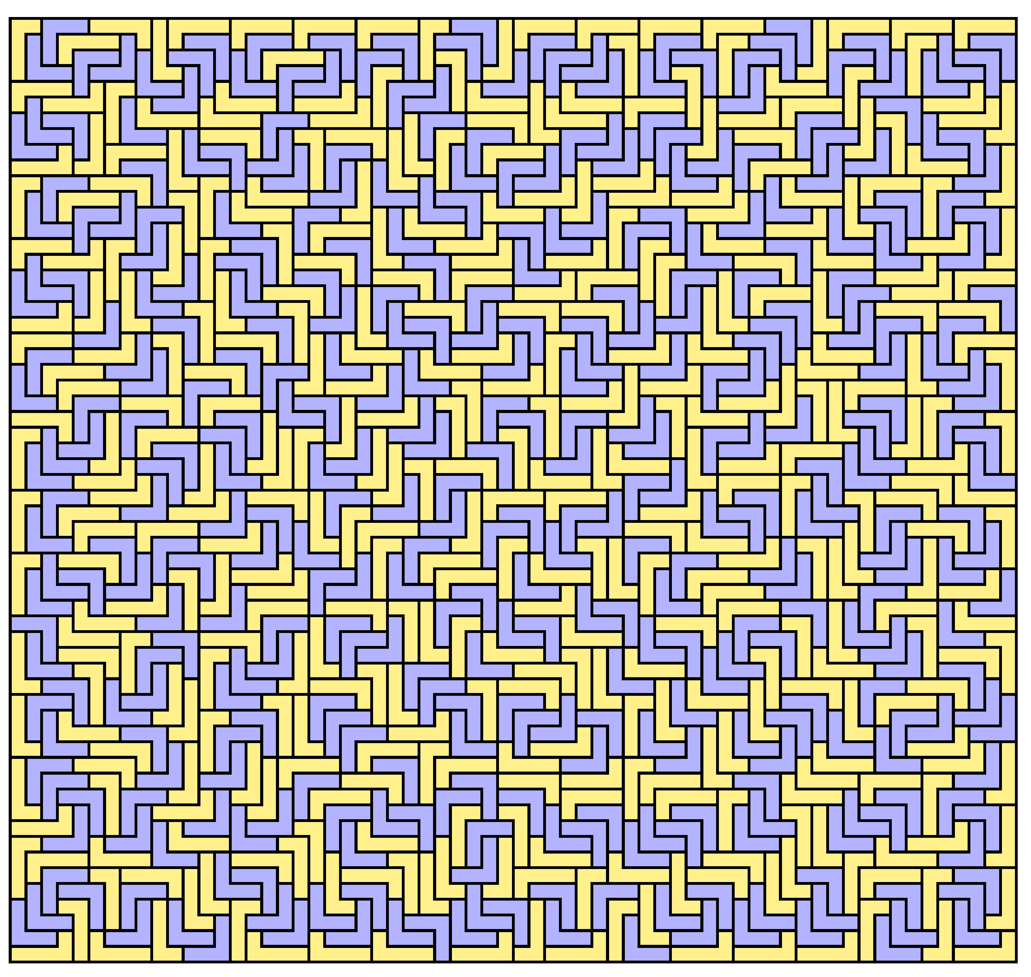
 all orientations permitted. We aim to tile R using= 384 copies of the V-shaped pentomino, and= 384 copies of the L-shaped pentomino. The associated ILP file, constructed with the program
LPMAKE_POLYOMINOES_FIGURE14, has n = 43,144 unknowns, m = 3842 constraints, and f = 39,303 free variables.
CPLEX
found an optimal solution in approximately 24 h.
all orientations permitted. We aim to tile R using= 384 copies of the V-shaped pentomino, and= 384 copies of the L-shaped pentomino. The associated ILP file, constructed with the program
LPMAKE_POLYOMINOES_FIGURE14, has n = 43,144 unknowns, m = 3842 constraints, and f = 39,303 free variables.
CPLEX
found an optimal solution in approximately 24 h. with parities, and 384 pariominoes from the set
 with parities, all orientations permitted. In the interests of space, we do not illustrate; however, it is sufficient to note that the top left square is white. The parity equation (see Theorem 1) is given by


